SHARMA & POOLE
488
UAJ2001
Symmetric Collaborative Filtering Using the Noisy Sensor Model
Rita Sharma
David Poole
Department of Computer Science
Department of Computer Science
University of British Columbia
University of British Columbia
Vancouver, BC V6T 1Z4
Vancouver, BC V6T 1Z4
rsharma@cs. ubc.ca
[email protected]
Abstract
used by Recommender Systems such as Amazon.com
Collaborative filtering is the process of mak ing recommendations regarding the potential preference of a user, for example shopping on
the Internet, based on the preference ratings
of the user and a number of other users for various items. This paper considers collabo rative filtering bMed on explicit multi-valued ratings. To evaluate the algorithms, we con sider only pure collaborative filtering, using ratings
exclusively, and no other information
about the people or items.
-a book store on the web, CDNow.com- a CD store on the web, and MovieFinder .com - a movie site on
the internet [Schafer, Konstan and Riedl, 1999]. Collaborative filtering (CF) is the process of making
predictions whether a user will prefer a particular item,
given his or her ratings on other items and given other people's ratings on various items including the one in question. CF relies on the fact that people's prefer ences are not randomly distributed; there are patterns within the preferences of a person and among simi
lar groups of people, creating correlation. The user for whom we are predicting a rating is called the ac
Our approach is to predict a user's prefer
tive user. In collaborative filtering, the main premise
ences regarding a particular item by using
is that the active user will prefer items which like
other people who rated that item and other
minded people prefer, or even that dissimilar people
items rated by the user as noisy sensors. The
don't prefer.
noisy sensor model uses Bayes' theorem to
a set of ratings for various user-item pairs, predict a
The problem can be formalized: given
compute the probability distribution for the
rating for a new user-item pair. It is interesting that
user's rating of a new item.
the abstract problem is symmetric between users and
We give two
variant models: in one, we learn a classical normal linear regression model of how users rate items; in another, we assume different users rate items the same, but the accuracy of the sensors needs to be learned. We com pare these variant models with state-of-the art techniques and show how they are sig
nificantly better, whether a user has rated only two items or many. We report empir ical results using the EachMovie database
1
of movie ratings. We also show that by con sidering items similarity along with the users similarity, the accuracy of the prediction in creases.
items. Collaborative filtering has been an active area of re search in recent years.
Several collaborative filter
ing algorithms have
suggested, ranging from bi
been
nary to non-binary rating, implicit and explicit rating. Initial collaborative filtering algorithms were based on statistical methods using correlation between user preferences [Resnick, Iacovou, Suchak, Bergstrom and Riedl, 1994; Shardanand and Maes, 1995]. These cor relation based algorithms predict the active user rat ings as a similarity-weighted sum of the other users ratings.
These algorithms are also referred to as
memory based algorithms [Breese, Heckerman and Kadie, 1998]. Collaborative filtering is different to the standard supervised learning task because there are
1
Introduction
Collaborative filtering is a key technology used to build Recommender Systems on the Internet. It has been
1http:/ /research.compaq.com/SRC/eachmovie/
only two attributes, each with a large domain; it is the structure within the domains that are important to the prediction, but this structure is not provided ex plicitly. Recently, some researchers have used machine learning methods [Breese et al., 1998; Ungar and Fos-
SHARMA & POOLE
UAI2001
ter, 1998) for collaborative filtering algorithms. These methods essentially discover the hidden attributes for users and items, which explain the similarity between users and items. Breese et al. [Breese et a!., 1998] proposed and eval uated two probabilistic models for model based col laborative filtering algorithms: cluster models and Bayesian networks. In the cluster model, users with similar preferences are clustered together into classes. The model's parameters, the number of clusters, and the conditional probability of ratings given a class are estimated from the training data. In the Bayesian net work, nodes correspond to items in the database. The training data is used to learn the network structure and the conditional probabilities. Lawrence and Giles, collaborative filtering algorithm
Pennock et al.[Pennock, Horvitz,
2000] proposed
a
called personality diagnosis (P D) and showed that PD makes better predictions than other memory and model based algorithms. This algor ithm is b ased on a probabilistic model of how people rate items, which is similar to our noisy sensor model approach.
In this paper we propose and evaluate a probabilis tic approach based on a noisy sensor model, which is symmetric between users and items. Our approach is based on the idea that to predict an active user's rating for a particular item, we can use all those people who rated that item and other items rated by the active user as the noisy sensors. We view the noisy sensor model as a belief network. The conditional probabil ity table associated with each sensor reflects the noise in the sensor. To model how another user (user u) can act as a noisy sensor for the active user a's rating, we need to find a relationship between their preferences. Unfortunately, there is usually very little data, so we need to make a priori some assumptions about the relationship. Here we give two variants of the general idea for learning the noisy sensor model for explicit multi-valued rat ing data: one, where we learn a classical normal lin ear regression model of how users rate items ( Noisyl) ; and another, where we assume that the different users rate items the same and learn the accuracy of the sen sor(Noisy2). In
order to avoid a perfect fit wi th sparse data we add some dummy points before fitting the relationship. We use hierarchical prior to distribute the effect of dummy points over all possible rating pairs. After learning the noisy sensor model (i.e. the con ditional probability table associated with each sensor node), we use Bayes' theorem to compute the proba bility distribution of the user a's rating of a new item.
489
We evaluate both Noisyl and Noisy2 on the Each Movie database of movie ratings and compare them to the state-of-the-art techniques. We also show that symmetric collaborative filtering, which employs both user and item similarity, offers better accuracy than asymmetric collaborative filtering. Filtering Problem and
2
Mathematical Notation
Let N be the number of users and M be the total num ber of items in the database. S is an N x M matrix of all user's ratings for all items; Sui is the rating given by user u to item i. Let the ratings be on a cardi nal scale with m values that we denote v1, v2, .. . , Vm· Then each rating Sui has a domain of possible values (v1,v2, , vm ) · In collaborative filtering, S, the user item matrix, is ge ner ally very sparse since each user will only have rated a small percentage of the total number of items. Under this formulation, the collabo rative filtering problem becomes predicting those Sui which are not defined in S, the user -item matrix. • . .
Collaborative Filtering Using the
3
Noisy Sensor Model
We propose a simple probabilistic approach for sym metric collaborative filtering using the noisy sensor model for predicting the rating by user a (active user) of an item j. We use as noisy sensors: •
all users who rated the item j
•
all items rated by user
a
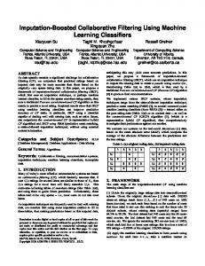
The sensor model is depicted as a naive Bayesian net work in Figure 1. The direction of the arrow shows that the prediction of user a for item j causes the sen sor u to take on a particular prediction for item j. The sensor model is the conditional probability table asso ciated with each sensor node. The noise in the sensor is reflected by the probability of incorrect prediction; that is, by the conditional probability table associated with it. To keep the model simple we use the indepen dence assumption that the prediction of any sensor for item j is independent of others, given the prediction of user a for item j. We need the following probabilities for Figure 1: P r (SuiiSaj) : the probability of user u's prediction for item j, given the prediction of user a for item j. Pr
(SakiSaj)
for item
k,
: the probability of user a's prediction given the prediction of user a for item j.
SHARMA & POOLE
490
UAI2001
to find a straight line which best fits these points. We assume that the mean of y can be expressed as a lin ear function of independent variable x. Since a model based on an independent variable cannot in general predict exactly the observed values of y, it is neces sary to introduce the error e;. For the ith observation, we have the following: y;
= a +
+ e;
(3x;
We assume that unobserved errors (e;) are indepen dent and normally distributed with a mean of zero
variance (]"2•
and the If Yi is the linear function of e;, which is normally distributed, then y; is also normally distributed. We as s ume the same variance for all the observations. T h e mean and variance of y; are given thus: Figure 1: Naive Bayesian Network Semantics for the Noisy Sensor Model
Pr (Saj) : the prior probabil ity of active
user a's pre
diction for item j.
We
the prior probability distribution of user a's rating for item j by the fraction of rating vi in the training data set, where ViE (vt,V2, . ..,vm ) ·
E (yi)
(3x;
= a +
var (y,)
==
(]"2
For th e ith observation, the probability distribution function of y which is normally distributed can be writ ten thus:
compute
Pr (Saj
=vi )
p (y where
=
y;Jx
,Ui
=
==
x;)
a+
==
(3x,
V2�a2 exp [ ;:.� (y;- ,u;)2]
Given the conditional probabilities table for all sen sors, we can comp ute the probability distribution for user a's rating of an unseen item j, using the noisy sensor model as described in Figure 1. By applying Bayes' rule we can have the following:
The joint probability distribution function ( or the like lihood function denoted by LF (a, (3, a2)) is the pr od uct of the individual P (y;lx;) over all observations.
Pr (Saj I (Slj, ... , SNj)
LF (a,j3,a2)
ex:
Pr (Saj)
N
. II
u=l
Pr
1\
(Sal, ... , SaM)) M
(Suj ISaj). II Pr (SakI Saj)
(1)
n =
IT P(y;Jx;)
=
k=l
To use the noisy sensor model for collaborative fil tering we need the probability table for probabilities: Pr(SuilSa.i) and Pr(Sa.k/Sa.J)· Consider first the problem of estimating Pr (Sui ISai ) , which is the problem of estimating user u's rating for item j given user a's rating of it. There is typically sparse data for the m x m probability table and we need to make some prior assumptions about the rela tionship. We assume that there is a linear relation ship with Gaussian error between the preferences of users and, similarly, between the ratings received by the items. Suppose the rating of user a (the indepen dent variable) is denoted by x, and t hat the rating of user u (the dependent variable) is denoted by y. Sup pose that user a and user u co- rated n it ems and their ratings over n co-rated items are denoted by n pairs of observations (xl,yl),(x2,Y2), ... ,(xn,Yn)- We want
We apply the maximum likelihood method [Gujarati, 1995] to estimate unknown parameters (a, (3, (]"2). The likelihood is maximum at the following values of the parameters: a==
1/n(LYi- f32:x;)
After calculating the parameters a, (3 and (]"2 we can write the expression of the probability distribution of user u's preference for item j given the user a's pref erence for it as follows: Pr
(Suj
= Xuj ISaj
=
Xaj)
=
P
(y
=
Xuj Jx
==
Xa.j)
UAI2001
SHARMA
1
=
� exp v 27fcr2
To estimate
[-1 (Xuj- (a+ /3Xaj))2] 2
u
Pr (SakiSaj),
We use the prior distribution of rating pairs for dis we use the same model as
case the independent variable
denotes the rating re
x
while dependent variable
. In this
y denotes
And, the n pairs of
the rating received by item k.
{xl,Yl), (x2,Y2), . . . , (xn,Yn) are the rat j and k by those n users, who have co-rated both items j and k. observations
ings over item
After
computing
Pr (SujiSaj) for and Pr (SakiSaj)
the
probability
all users
(u)
for all items
(k)
distribution
who rated item
j,
rated by user a, we
can compute the probability distribution of the user a rating for item j using Equation we need to compute and (!2
),
We compute the prior distribution of
each rating pair by its frequency in the training data.
Pr (Suj ISaj)
j,
491
rating pairs.
2
described above for computing ceived by item
& POOLE
3 * ( u + i)
(1).
In this model
free parameters
(a,
{3,
where u is the number of users who rated
the item j and i is the number of items rated by user
a.
tributing the effect of K dummy points over all rating pairs like hierarchical
prior.
be distributed over all possible rating pairs. We have experimented with parameter K, and we found that
Noisyl
performs better with K = 1. For subsequent
experiments we, therefore, chose K = 1 for
3.2
Noisyl.
S e lec t i ng Noisy Sensors
For determining the reliability of the noisy sensors, we consider the
goodness of fit of
the fitted regression
line to a set of observations. We use the coefficient of determination
r2
[Gujarati, 1995], a measure that tells
how well the regression line fits the observations. This coefficient measures the proportion or percentage of the total variation in the dependent variable explained by the regression model.
When the linear relationship exceeds the maximum
This, however, reduces
our ability to guarantee the ratings for K items will
r2
is calculated as follows
[Gujarati, 1995}:
value of the rating scale, we use the maximum value; when it is lower than the minimum value of the rating scale, we use the minimum value.
=
To predict a rating (for example, to compare it with
1-
"'"'e2 L., �
� (Yi- fJ)2
other algorithms that predict ratings), we predict the
where y is the mean of the ratings of user u.
expected value of the rating.
The value of
The expected value of
the rating is defined as follows:
E (Saj) =
is, e;
(Slj, ... , SNi) I\ (Sal, ... , SaM).
lies b etween 0 and 1 ( 0 ::; r2 ::; 1) .
=
0 for each observation (co-rated item).
r2
=
On
0, it means there is no linear
is horizontal line going through the mean y. We order
find a perfect linear relationship, even though the sen sor isn't perfect. If there is a perfect fit between users a and u, then the variance will be zero according to the above calculations. Therefore, the sensor u's predic
tion for item j will be perfect, or deterministic; that is,
the conditional probability table associated with sen We do not want
this for our noisy sensor model because a determinis tic sensor will discount the effects of other sensors. For example, often one or two co-rated items always have a perfect fit, even though such a user is not a good sensor.
the user and item noisy sensors according to
r2.
We
use the best U user noisy sensors and best I item noisy sensors for making the predictions.
The parameter
settings for U and I are explained in the next section.
3.3
Variant Noisy2 of Noisyl
The problem with
Noisyl is that
we must often fit lin
ear relationships with very little data (co-rated items). It may be better to assume a priori the linear model and then simply learn the noise. The algorithm
Noisy2
is based on the idea that different users rate items the same and, similarly, different items receive the same rating. We assume that the preferences of user a and
We hypothesize that this problem can be overcome if we add K dummy observations along with n obser vations (co-rated items). We assume that user u
r2
1, there exists a perfect linear relationship
relationship between users a and u and the best fit line
While trying to fit Jines with sparse data, we often
user
=
the other hand, if
K Dummy Observations
sor u will be purely deterministic.
r2
between the preferences of user a and user u; that
�;:1 Pr (Saj =Vi IX)* Vi
where X=
3.1
If
a
and
user u are the same; that is, the expected value of user
u's preference of any item is equal to active user a's preference for th at item.
give ratings over K dummy items (K > 0) in
E
such a way that their ratings for K dummy items are distributed over all possible rating pairs. For m scale
rating data there are
m2
possible combination of the
(Yilx = x;)
= 11 =
x;
We learn the variance of user u's prediction. The al gorithm
Noisy2 can be
derived from algorithm
Noisyl
492
SHARMA & POOLE
by making the regression coefficients a = 0 and /3 = 1. In this model we need to compute (u + i) free param eters (a2), where u is the number of users who rated the item j and i is the number of items rated by user a. We also add the K dummy observations because the same problem (as discussed in Subsection 3.1) can arise in Noisy2. We have experimented with parame ter K, and we found that Noisy2 also performs better with K 1. For subsequent experiments we, there fore, chose K = 1 for Noisy2 also. =
In Noisy2 we are not fitting the relationship between user a and user u, but we assume an equal relation ship. So, it doesn't make sense to use the coefficient of determination r2 for finding the reliability of the noisy sensors. Rather, to find the reliability of the noisy sen sor, we use the variance; the less variance, the more reliable the noisy sensor. We use the best U user noisy sensors and best I item noisy sensors for making the predictions. The parameter settings for U and I are explained in the next section.
4
Evaluation Framework
To evaluate the accuracy of collaborative filtering al gorithms we used the training and test set approach. In this approach, the dataset of users (and their rat ings) is divided into two: a training set and a test set. The training set is used as the collaborative filtering dataset. The test set is used to evaluate the accuracy of the collaborative filtering algorithm. We treat each user from the test set as the active user. To carry out testing, we divide the ratings by each test user into two sets: Ia and Pa. The set Ia contains ratings that we treat as observed ratings. The set Pa contains the rat ings that we attempt to predict using a CF algorithm and observed ratings (Ia) and training set. To evaluate the accuracy of the collaborative filtering algorithm we use the average absolute deviation met ric, as it is the most commonly used metric [Breese et al., 1998]. The lower the average absolute deviation, the more accurate the collaborative filtering algorithm is. For all users in the test set we calculate the average absolute deviation of the predicted rating against the actual rating of items. Let the number of predicted ratings in the test set for the active user be na; then the average absolute deviation for a user is given as follows:
Sa=
,;, LjEPa IPa,j- ra,jl,
where Pai is user a's observed rating for item j and raj is user a's predicted rating for item j. These absolut e deviations are users in the test set.
then averaged over all
4.1
UAI2001
Data and protocols
We compared both versions of our noisy sensor model to PD (Personality Diagnosis) [Pennock et al., 2000] and Correlation (Pearson Correlation) [Resnick et al., 1994]. To compare the performance we used the same subset of the EachMovie database as used by Breese et al. [Breese et al., 1998] and Pennock et al. [Pennock et al., 2000], consisting of 1,623 movies, 381,862 rat ings, 5,000 users in the training set, and 4,119 users in the test set. In EachMovie database the ratings are elicited on a integer scale from zero to five. We also tested the algorithms on other subsets to verify that we are not finding peculiarities of the subset. We ran experiments with different amounts of ratings in set Ia to understand the effect of the amount of the observed ratings on the prediction accuracy of the collaborative filt ering algorithm. As in [Breese et al., 1998] for the AllBut1 Protocol, we put a sin gle randomly selected rating for each test user in the test set Pa and the rest of the ratings in the observed set I