MARINE ECOLOGY PROGRESS SERIES Mar Ecol Prog Ser
Vol. 517: 85–104, 2014 doi: 10.3354/meps11024
Published December 15
Temperature effects on Calanus finmarchicus vary in space, time and between developmental stages Kristina Øie Kvile1,*, Padmini Dalpadado2, Emma Orlova3,†, Nils C. Stenseth1, Leif C. Stige1 1
Centre for Ecological and Evolutionary Synthesis (CEES), Department of Biosciences, University of Oslo, PO Box 1066 Blindern, 0316 Oslo, Norway 2 Institute of Marine Research, PO Box 1870 Nordnes, 5817 Bergen, Norway 3 Knipovich Polar Research Institute of Marine Fisheries and Oceanography, Knipovich-St. 6, 183763 Murmansk, Russia
ABSTRACT: Temperature is considered one of the major factors shaping marine zooplankton distribution, abundance and phenology. During the past decades, the Barents Sea experienced strong temperature fluctuations, but previous studies have not identified a clear link between temperature and the dynamics of the key copepod species Calanus finmarchicus. We investigated associations between regional and local water temperature and C. finmarchicus abundance in Atlantic waters of the Norwegian and Barents Seas between 1959 and 1992. Results differed depending on the developmental stage, season and area, emphasising the value of detailed data series in climate effect studies. Abundances of copepodite stage CV and adult females showed no strong correlations with regional temperature indices, but were positively linked to local temperature in both spring and summer. For nauplii and young copepodite stages (CI−CIV), associations with both regional and local temperature estimates were positive in spring, but negative in summer. The results indicate that the phenology of young copepodites may be particularly responsive to climate change, which in turn may influence predators feeding on these life stages. KEY WORDS: Barents Sea · Copepod · Climate change · Generalised additive models · Norwegian Sea · Seasonality · Temperature · Zooplankton Resale or republication not permitted without written consent of the publisher
INTRODUCTION Temperature is believed to be the most important factor structuring marine ecosystems (e.g. Richardson 2008, Hoegh-Guldberg & Bruno 2010), and warming of the oceans due to climate change is currently altering a wide range of marine ecosystem properties (e.g. production, species composition and seasonal timing; Pörtner et al. 2014). By virtue of a combination of factors, zooplankton are thought to be ideal climate indicators (Richardson 2008). For example, as zooplankton are poikilothermic, physiological processes such as growth and reproduction are tightly coupled to temperature variation. The short life span of most zooplankton (often less than 1 yr) *Corresponding author:
[email protected] † Deceased
allows a quick response in population dynamics to climatic variation. Furthermore, since few zooplankton species are to date commercially harvested, effects of climate variation are less likely to be confounded with effects of fishing than in many other marine groups. Effects of temperature variability have been reported on zooplankton distribution, species composition, abundance and phenology (seasonal development) (Edwards & Richardson 2004, Richardson 2008). Zooplankton populations typically display pronounced seasonality correlated with variation in temperature or other external factors (e.g. photoperiod, phytoplankton production), particularly in high-latitude areas where food availability is re© Inter-Research 2014 · www.int-res.com
86
Mar Ecol Prog Ser 517: 85–104, 2014
stricted to a short time window (Eiane & Tande 2009, Mackas et al. 2012). Observed alterations in phenology have often been correlated with temperature, typically with seasonal processes occurring earlier during warmer years (Orlova et al. 2010, McGinty et al. 2011, Mackas et al. 2012). Climate change can affect marine plankton phenology differently across functional groups and trophic levels (Edwards & Richardson 2004). In this study, we demonstrate how temperature variation might affect a zooplankton species differently depending on the geographical area, season and developmental stage. The Barents Sea is a highly productive subarctic shelf sea, in particular in southwestern areas adjacent to the Norwegian Sea, and plankton represent the bulk of animal production (Sakshaug et al. 2009). Calanus finmarchicus is the dominant copepod species in the Atlantic water masses in the Norwegian and Barents Seas (Melle et al. 2004, Eiane & Tande 2009, Orlova et al. 2010). In the Norwegian Sea, north of 68°N, C. finmarchicus usually has a 1 yr life cycle, during which it develops through 6 nauplii stages (NI−NVI) and 5 copepodite stages (CI−CV) to the adult stage (CVI) (Eiane & Tande 2009). By the end of the growth season (late summer), older stages (mainly CV, but also CIV and CVI; Melle et al. 2004) descend to deeper waters to over-winter. When adults return to the surface in spring to feed on phytoplankton and spawn, the life cycle is completed. C. finmarchicus is the primary food source for many fish species, including Northeast Arctic cod larvae that prey on nauplii and young copepodite stages (Ellertsen et al. 1987, 1989, Karamushko & Karamushko 1995). The Barents Sea experienced alternating cold and warm periods during the second half of the 20th century, with a warming trend dominating since the 1980s (Johannesen et al. 2012). Although spatial and temporal variation in zooplankton biomass has been observed (e.g. Dalpadado et al. 2012, Johannesen et al. 2012), long-term data series to study the effect of climatic variability on copepod dynamics have been scarce (Tande et al. 2000, Eiane & Tande 2009), and several previous studies in the Barents Sea did not identify a clear association between temperature variation and the dynamics of C. finmarchicus (Tande et al. 2000, Stige et al. 2009, 2014, Dalpadado et al. 2012). Note, however, that the data analysed in these studies were limited to the upper water layer (0−50 m depth) (Tande et al. 2000, Stige et al. 2009), a few selected years (Tande et al. 2000) and/or aggregated biomass data (Stige et al. 2009, 2014, Dalpadado et al. 2012).
A notable exception, the Knipovich Polar Research Institute of Marine Fisheries and Oceanography (PINRO, Murmansk, Russia) collected zooplankton data during their ichthyoplankton surveys in the Norwegian and Barents Seas between 1959 and 1993. Some of these data have previously been analysed, with results available in Russian (Degtereva 1973, 1979, Antipova et al. 1974, Degtereva et al. 1990, Nesterova 1990, Drobysheva & Nesterova 2005; Tande et al. 2000 also analysed some of these data). Analyses of data from the Kola section (along 33.5°E) showed a positive association between temperature and zooplankton biomass in spring during the 1960s (Antipova et al. 1974), and earlier plankton development during warmer years when 8 yr of contrasting temperatures in the 1970s and 1980s were compared (Drobysheva & Nesterova 2005). The Russian survey data on both ichthyoplankton and zooplankton have recently been digitised, and we here report on the first analyses of the complete dataset of C. finmarchicus stage-specific abundance. The data cover both shelf areas in the Norwegian and Barents Seas where variation in Atlantic water inflow is believed to be a main regulator of C. finmarchicus biomass (Helle & Pennington 1999, Dalpadado et al. 2003, Edvardsen et al. 2003a), and Norwegian Sea off-shelf areas considered as sources of C. finmarchicus to the shelves (Slagstad & Tande 1996, 2007, Halvorsen et al. 2003, Edvardsen et al. 2006). The long time span, high spatial resolution and coverage, region (subarctic) and separation into developmental stages make this dataset unique among climate effect studies on zooplankton (Richardson 2008, Mackas et al. 2012). Using spatiotemporal statistical analyses, we investigated associations between temperature and C. finmarchicus abundance, separating responses to temperature between different developmental stages, depths, seasons and geographical areas. This enabled us to shed light on whether temperature effects act primarily on abundances, vertical distribution or phenology.
MATERIALS AND METHODS Zooplankton data Zooplankton data were collected by PINRO during their ichthyoplankton surveys in spring (April−May) and summer (June−July) between 1959 and 1993. Sampling methods are described by Nesterova (1990). In brief, plankton samples were collected in the northeastern Norwegian Sea and southwestern
Kvile et al.: Temperature effects on Calanus finmarchicus
87
Fig. 1. (A) Study region (dashed area) with depth contours at every 500 m. (B−D) Distribution of sampling stations with stagespecific Calanus finmarchicus abundance data (n = 5026) by (B) geographical position, (C) depth layer (Upper: upper sampling depth ≤20 m and lower sampling depth ≤60 m, Middle: upper sampling depth 40–60 m and lower sampling depth ≤120 m, Lower: upper sampling depth > 90 m) and (D) year. In (B), the size of the mapped circles reflects the number of times a station was sampled during the period 1959 to 1992. The positions of the Skrova station and the Kola section are marked with a red triangle and a red dashed line, respectively
Barents Sea along specific transects and depth layers (Fig. 1). The gear used was a Juday plankton net (37 cm diameter opening, 180 µm mesh size) with a closing mechanism, towed vertically from the lower depth to the upper depth of the sample. The main component of zooplankton biomass in the area and the dataset is Calanus finmarchicus (Nesterova 1990). For a total of around 5000 samples, specimens of this species were recorded as stage-specific abundance, expressed as ind. m−3, accounting for the opening area of the net and the depth hauled. While nauplii are difficult to determine to species and were recorded as Calanus sp., C. finmarchicus copepodites (CI−CV) and adult males and females (CVI-
M and CVI-F) were discriminated from other calanoid copepods. There was some year-to-year variation in the stations sampled and depths hauled, particularly during the early years of the programme. In some years, sampling effort was reduced (specifically, no samples were collected in spring 1967, and no stage-specific counts were recorded in 1990 or 1993). All samples were in the dataset described by an ‘upper sampling depth’ (i.e. the shallowest depth of the vertical haul) and a ‘lower depth’ (i.e. the bottom of the haul). In most cases, the depths hauled fell within these 3 depth categories: 0–50 m, 50–100 m and 100 m– bottom. However, some samples deviated from this
88
Mar Ecol Prog Ser 517: 85–104, 2014
Table 1. Model equations describing general patterns of Calanus finmarchicus scheme. In order to encompass as abundance (Eqs. 1 & 2) and temperature associations in abundances (Eqs. 3−6). many samples as possible, we formuZ: stage-specific abundance, β: intercept, s( j): smooth function of day-of-year, lated the following new depth cates(d): smooth function of average sampling depth, te(x,y): 2-dimensional tensor gories: Upper: upper sampling depth product of longitude and latitude, l: indicator variable of season (spring or summer), s(Y ): random effect of year, ε: random error, te(x,y,j): 2-dimensional ≤ 20 m and lower sampling depth ≤60 tensor product of longitude and latitude (2-dimensional smooth) and day-ofm (n = 3578); Middle: upper sampling year (1-dimensional smooth), s(T ): smooth function of temperature anomaly, T: depth 40–60 m and lower sampling linear function of temperature anomaly. See Supplement 1 at www.int-res. depth ≤120 m (n = 724); Lower: upper com/articles/suppl/m517p085_supp.pdf for further details on model terms sampling depth > 90 m (n = 724). Less than 5% of the samples were exModel Equation Eq. cluded when using these categories number (n = 256). These were mainly samples General covering a large depth interval (e.g. Spatial, seasonal and Z = β + s( j) + s(d) + te(x,y)l + s(Y ) + ε 1 from the surface to several hundred vertical variation meters), but also some samples falling Interaction between position Z = β + te(x,y,j) + ε 2 and day of year between the set intervals (e.g. from 30 to 60 m) or with missing depth Temperature effects Simple temperature effect Z = β + s( j) + s(d) + te(x,y)l + s(T ) + ε 3 information. Seasonally varying Z = β + s( j) + s(d) + te(x,y)l + s(T )l + ε 4 Due to their small size, nauplii are temperature effect under-sampled by the mesh size used Spatially varying Z = β + s( j) + te(x,y)l + te(x,y)lT + ε 5 (Hernroth 1987, Nichols & Thompson temperature effect 1991). Considering this, in addition to Spatially and temporally Z = β + te(x,y,j)+ te(x,y,j)T + ε 6 varying temperature effect the uncertainties in species determination of nauplii, we therefore present results for total nauplii abunaging observations from the months December (from dances only (N total), which should be interpreted the previous year) to February (Winter index), March with caution. Abundances of adult males (CVI-M) to May (Spring index) and June to August (Summer were 0-inflated; 60% of the samples contained no index). To study associations between C. finmarchimales, compared to 25% for females (CVI-F) and cus abundance and local temperature variation 10−20% for nauplii and copepodite stages. C. (spatially and seasonally), we used temperature estifinmarchicus males are known to appear earlier than mates corresponding to the date (day, month, year) females after overwintering, and die off sooner after and position (latitude, longitude) of samples from a fertilisation (Melle et al. 2004). As the data indicated numerical ocean model hindcast archive (Lien et al. that the spring survey was too late to sample males 2013). The model domain includes the Nordic Seas during their main appearance, the abundance data and the Barents Sea back to 1959 at 4 km resolution, on adult males (CVI-M) were not included in the and it realistically represents the variability in the analyses of temperature associations described Atlantic water masses in the zooplankton survey area below. (Lien et al. 2013). Three depth-integrated temperature indices were calculated per station by averaging local temperature estimates from 0, 10, 20 and 50 m Ocean temperatures (Upper), 50 and 100 m (Middle) and 100 and 250 m (Lower). Local temperature anomalies were calcuTo assess associations between year-to-year varialated by extracting the residuals from a generalised tion in C. finmarchicus abundance and regional temadditive model (GAM, Hastie & Tibshirani 1990, perature, we used monthly mean sea temperature Wood 2006) where the local temperature index observations from the Kola section (along 33.5°E in described above was modelled as a function of posithe Barents Sea, 0−200 m depth) provided by PINRO tion, day-of-year and depth layer (see Eq. S1 in Sup(Tereshchenko 1996), and monthly temperature obplement 1 at www.int-res.com/articles/suppl/m517 servations from the Skrova station in Vestfjorden, p085_supp.pdf). These local temperature anomalies Lofoten Islands (68.1°N, 14.7°E, 0−200 m; Institute of can be interpreted as deviances from the expected Marine Research, Aure & Østensen 1993) (Fig. 1B). temperature at the position, day-of-year and depth of Vertically averaged (0−200 m) seasonal indices of a zooplankton sample. these 2 temperature series were calculated by aver-
Kvile et al.: Temperature effects on Calanus finmarchicus
General patterns of C. finmarchicus abundance Year-to-year variation in C. finmarchicus abundance was assessed by constructing year- and season-specific indices of stage-specific abundances. These seasonal abundance indices were constructed by extracting year-specific intercepts from a GAM formulated separately for spring and summer samples, where the natural logarithm of observed stagespecific abundances (with 1 added to avoid taking the logarithm of 0) was a function of day-of-year, sampling depth and location (Eq. S2 in Supplement 1). The indices can be interpreted as mean stagespecific abundances for a given season and year, taking into account year-to-year variability in sampling stations (both in time and space). Spatial, seasonal and vertical variation in abundance was explored by fitting GAMs where observed stagespecific abundances (loge[n + 1]) were a function of location, day-of-year and depth (Eq. 1 in Table 1). The effect of location could vary between spring and summer, defined as the transition between May and June (Day-of-year 150). An alternative version of Eq. (1) where the effect of depth on abundance could vary with season was formulated to investigate whether vertical distribution patterns differed between spring and summer (Eq. S3 in Supplement 1). We hypothesised that seasonal variation in abundances might differ geographically (e.g. earlier appearance in the southern parts of the surveyed area; Manteufel 1941, Loeng & Drinkwater 2007). To visualise seasonal variation in abundances in different areas, we extracted model predictions from an alternative model (Eq. 2 in Table 1) where the effects of geographical position and day-of-year interact. Predicted abundances from late April (Day 115) to midJuly (Day 194) in the upper water layer (lower sampling depth ≤60 m) were computed for 3 locations: (1) off-shelf in the northeastern Norwegian Sea (69.7°N, 15.0°E), (2) in the Barents Sea entrance south of Bjørnøya (72.7°N, 19.5°E) and (3) in the Barents Sea proper (73.0°N, 30.5°E).
Associations with temperature Associations between stage-specific abundances and regional temperature were quantified by calculating the Spearman rank correlation coefficient (rS) between seasonal abundance indices and temperature indices from the Kola section and Skrova station. To account for autocorrelation in the time series, the effective number of degrees of freedom in the signif-
89
icance test for the correlation was adjusted according to the method described by Quenouille (1952) and modified by Pyper & Peterman (1998). Associations between stage-specific C. finmarchicus abundances and local temperature anomalies were investigated with statistical analyses (GAMs) of spatially and temporally resolved observation data. Before the analyses, the observation data were assigned to 1 of the 3 depth categories decscribed in ‘Zooplankton data’ above: upper, middle or lower. GAMs with various levels of complexity (Eqs. 3−6 in Table 1, Eq. S4 in Supplement 1) were investigated to address how associations between local temperature anomalies and stage-specific abundances of C. finmarchicus (1) differ between developmental stages, depths and seasons, (2) differ between different geographical areas and (3) shape variation in abundances throughout the spring and summer seasons. (1) Simple additive temperature effect. In the simplest case, we assumed that temperature has a similar additive effect on abundances (loge [n + 1]) across space and time (Eq. 3 in Table 1). The first part of the model formulation corresponds to the first part of Eq. (1) and constitutes the null-model to which a smooth function of local temperature anomaly was added (see Supplement 1 for further details). Further, to investigate whether the temperature effect differed seasonally and between depth layers, we added a factor variable of season (Eq. 4 in Table 1) and depth (Eq. S4 in Supplement 1) to the temperature term. The following more complex models were only explored for samples from the surface layer, corresponding to the depth layer with the highest abundances during the growth season (Tande 1988b, Dale & Kaartvedt 2000, this study). (2) Spatially varying temperature effect. To investigate whether the association between temperature and abundance differs between areas, we explored spatially varying coefficient models (Hastie & Tibshirani 1993), where the effect of temperature is assumed to be linear at any given location, but the slope of the temperature term can change smoothly and non-linearly in space and can differ between seasons (Eq. 5 in Table 1). Site-specific predictions of the temperature term were extracted, and significantly positive slope coefficients (for which the 2.5% percentile of the bootstrap distribution of the slope value was > 0) or significantly negative slope coefficients (for which the 97.5% percentile of the bootstrap distribution was < 0) were mapped. The bootstrap procedure is explained in the final paragraph below.
Mar Ecol Prog Ser 517: 85–104, 2014
90
General dynamics in C. finmarchicus abundance
(3) Spatially and temporally varying temperature effect. To further investigate whether, and how, zooplankton phenology is influenced by temperature, and how this varies across areas, the temperature effect was modelled as a linear function varying smoothly with both geographical position and day-ofyear (Eq. 6 in Table 1). Predicted daily abundances from late April (Day 115) to mid-July (Day 194) in the 3 locations previously described (see ‘General patterns of C. finmarchicus abundance’ above) were extracted for a colder-than-average scenario and a warmerthan-average scenario. For the colder scenario, temperatures were set to be 1°C below the expected temperature for a given time and position (i.e. temperature anomalies = −1), and for the warmer scenario, temperatures were set at 1°C above the expected (i.e. temperature anomalies = +1). The different models (Eq. 1−6 in Table 1) were compared to null-models, only accounting for spatiotemporal variation in the data with genuine crossvalidation (GCV), a measure of predictive power, and R2, a measure of the proportion of data variation explained by the model. For the comparison, models were only fitted for data from the upper water layer, not including the effect of sampling depth. To account for within-year spatial autocorrelation which might lead to erroneous identification of significant effects (Zuur et al. 2007), 95% confidence intervals of the model effects were computed for all model formulations using nonparametric bootstrapping (1000 samples with replacement) with year as the sampling unit (Hastie et al. 2009). Further details on the calculation of GCV and model comparison are given in Supplement 2 at www.int-res.com/articles/suppl/ m517p085_supp.pdf. All analyses were implemented in R (R Development Core Team 2014), using the mgcv library for GAMs (Wood 2013).
Stage-specific abundances fluctuated throughout the years of the survey, without displaying any clear upward or downward trends (Fig. 3). The seasonal variation in abundances from spring to summer displayed a transition between increasingly older developmental stages throughout the spring and summer. On average, abundances of nauplii and stages CI−CII were higher in spring than summer, while the opposite was found for stages CIII−CV (Fig. 3). Abundances of CVI-F were generally higher in spring than summer, while CVI-M were only present in low abundance in both seasons. Predicted abundances from early spring to late summer in the upper water layer (Eq. 2 in Table 1) for a selected Norwegian Sea location (69.7°N, 15.0°E) indicated that abundances of nauplii and stages CI−CIII generally peaked during (or possibly before) the early parts of the spring survey, with indications of a second peak during late summer (Fig. 4, Location 1). Abundances of CIV, CV and CVI-F were relatively stable or increased throughout spring and summer. The seasonal dynamics were delayed in locations farther north and east in the surveyed area (Fig. 4, Locations 2 and 3), where abundances of nauplii remained higher during the surveyed period than in the southernmost location (but also decreased); CI−CIII seemed to peak around the transition between spring and summer (Day 150), and CIV and CV peaked later in summer, or possibly after the summer survey. In Locations 2 and 3, CVI-F were present in low abundance during the surveyed period. CVI-M were present in low abundance in Locations 1 and 2, and nearly absent in Location 3.
RESULTS
Spatial variation
Temperature variation
The spatial variation of C. finmarchicus stagespecific abundances is illustrated in Fig. 5 as predicted abundances per position (Eq. 1 in Table 1) at median sampling depth (28 m) and median sampling day in spring (Day 129: 9 May) and in summer (Day 175: 4 July). In spring, the highest abundances of nauplii and stages CI−CIII were generally found off the Norwegian coast and in the southern Barents Sea, while in summer, the distribution centre was relocated farther north in the Norwegian and Barents Seas. Abundances of CIV were highest in the Norwegian Sea and the Barents Sea entrance in spring, with a shift to in-
Ocean temperature measurements from the Kola section and Skrova station fluctuated over the years of the study, with a cold period in the late 1970s, and generally increasing temperatures since the 1980s (Fig. 2) (as described by Johannesen et al. 2012). The local temperature estimates for the surveyed area generally increased from spring to summer, with highest temperatures occurring in the Norwegian Sea coastal areas compared to open Norwegian Sea and Barents Sea areas.
Temporal variation
Kvile et al.: Temperature effects on Calanus finmarchicus
91
Fig. 2. Spatiotemporal variation in temperature during the course of the study. Local temperature estimates (°C) at the survey stations (see Fig. 1B), averaged over the years 1959 to 1992 and 0 to 250 m depth, in (A) spring and (B) summer. Year-to-year variation in temperature indices (°C) from the Kola section (solid line) and Skrova station (dashed line) in (C) spring and (D) summer. Local temperature estimates were interpolated in space using a generalised additive model with local temperature as a function of a tensor product smooth of longitude and latitude. See ‘Materials and methods’ for calculation of regional temperature indices
creased abundances in the Barents Sea in summer. There was less seasonal difference in the spatial distribution of stages CV and CVI-F, which were found in higher abundances in the Norwegian Sea than in the Barents Sea in both spring and summer. Stage CVIM were found primarily in the Norwegian Sea area.
Supplement 3). The influence of position, day-of-year and sampling depth on stage-specific abundances is shown in Table S1 in Supplement 3.
Vertical variation
Regional temperature
Abundances of all stages were highest in the upper 50 m and decreased in deeper water (Fig. S1 in Supplement 3 at www.int-res.com/articles/suppl/m517 p085_supp.pdf), although stages CIV, CV and CVI-F also showed a slight increase in abundances from around 100 to 200 m. An alternative model with a seasonally varying depth effect (Eq. S3 in Supplement 1) indicated that this second peak was more pronounced in summer than in spring (Fig. S2 in
Correlations between seasonal abundance indices of nauplii and copepodite stages CI−CIV and Kola and Skrova temperatures were generally positive in spring and negative in summer (Table S2 in Supplement 3). Statistically significant correlations were identified for stages CII−CIV in spring and summer and for stage CI in summer. No significant correlations were observed between regional temperature indices and abundances of stages CV or CVI-F.
Associations between temperature and C. finmarchicus abundance
92
Mar Ecol Prog Ser 517: 85–104, 2014
Fig. 3. Year-to-year variation in Calanus finmarchicus stage-specific seasonal abundance indices (loge[n + 1]) in spring (solid lines) and summer (dashed lines). Abundance indices are year-specific intercepts from Eq. S2 in Supplement 1 at www.intres.com/articles/suppl/m517p085_supp.pdf. The vertical lines mark the nominal 95% confidence interval (not accounting for spatial autocorrelation) of the abundance indices (solid lines for spring, dashed lines for summer). Also displayed are, per developmental stage, the overall mean and standard deviation of the spring and summer indices. N total: total nauplii abundance, CI−CVI: stage-specific copepodite abundances; M: male; F: female
Local temperature anomalies (1) Simple additive temperature effect. In the simplest case (Eq. 3 in Table 1), we assumed that the effect of temperature variation on abundance does not
change across space or in time but can differ between developmental stages. The results indicated a weakly positive but non-significant temperature effect on abundances of nauplii and stages CI−CIV, and a significant positive association for stages CV
Kvile et al.: Temperature effects on Calanus finmarchicus
Fig. 4. Predicted abundances (plots) of Calanus finmarchicus developmental stages (loge[n + 1]) throughout the spring and summer seasons in 3 locations (map): 1 (left column), off-shelf in the north-eastern Norwegian Sea (69.7° N, 15.0° E); 2 (centre column), in the Barents Sea entrance south of Bjørnøya (72.7° N, 19.5° E); and 3 (right column), in the Barents Sea proper (73.0° N, 30.5° E). Predictions were extracted from Eq. 2 in Table 1, based on pooled data from the upper water layer for the period 1959 to 1992. Shaded area: 95% confidence interval from bootstrap procedure. Grey dots: sampled stage-specific abundances (loge[n + 1]) from stations within 50 km of each location. N total: total nauplii abundance, CI−CVI: stagespecific copepodite abundances; M: male; F: female
93
94
Mar Ecol Prog Ser 517: 85–104, 2014
Fig. 5. Predicted stage-specific abundances (loge[n + 1], Eq. 1) of Calanus finmarchicus in the study area in spring and summer, at averaged values for sampling depth (28 m) and day-of-year (spring, Day 129: 9 May; summer, Day 175: 4 July), based on pooled data for the period 1959 to 1992. The numbered isolines mark the predicted stage-specific abundances, from green areas with the relatively lowest abundances, to orange/red areas with the relatively highest abundances. Note that model predictions are more uncertain for areas with low data coverage (see Fig. 1B). N total: total nauplii abundance, CI−CVI: stagespecific copepodite abundances; M: male; F: female
and CVI-F (Fig. 6, left). However, when we let the temperature effect differ between spring and summer (Eq. 4 in Table 1), a more detailed picture emerged. Positive temperature anomalies were associated (1) with above-average abundances of nauplii and CI−CIV in spring, (2) with below-average abundances of these stages in summer and (3) with aboveaverage abundances of CV and CVI-F in both spring and summer (Fig. 6, middle and right). The associations for CIV−CV in summer did not significantly differ from 0 (the 95% confidence interval of the additive effect surrounded 0). We found few indications of a differing effect of temperature with depth
(Fig. S3 in Supplement 3). The confidence intervals for the temperature effects in different depth layers were generally overlapping, with a possible exception of nauplii and CI−CIII in summer, for which the negative association with temperature was only observed in the upper water layers. Based on these findings, we proceeded with the more complex model investigations looking only at temperature effects on abundance in the upper water layer. (2) Spatially varying temperature effect. Slope coefficient values from a spatially varying coefficient model (Eq. 5 in Table 1) mapped per sampling position (Fig. 7) reflected the seasonal patterns from the
Kvile et al.: Temperature effects on Calanus finmarchicus
95
Fig. 6. Additive effect of local temperature anomalies on Calanus finmarchicus stage-specific abundances (loge[n + 1]). Left column: additive temperature effect estimated for spring and summer combined (Eq. 3 in Table 1). Centre and right columns: additive effect estimated for spring and summer separately (Eq. 4 in Table 1). Shaded area: 95% confidence interval from bootstrap procedure. Dashed line: 0 effect isoline. Stars indicate a significant association, i.e. that the effect differs from 0 in parts of the covariate’s range. N total: total nauplii abundance, CI−CVI: stage-specific copepodite abundances; F: female
simple additive model (Fig. 6), but displayed some spatial variation in the strength of the temperature association. For nauplii, the positive association in spring was restricted to west of around 24°E, and the negative association in summer to the east of
this border. The largest spatial extent of significant temperature associations was found for stages CI−CIII, with significant positive associations in spring in most of the survey area (except the northernmost transects for CI and CIII). Negative associa-
96
Mar Ecol Prog Ser 517: 85–104, 2014
(Figure continued on next page)
Fig. 7. Significantly negative (blue) or positive (red) slope coefficients for a linear temperature effect on Calanus finmarchicus stage-specific abundances (Eq. 5 in Table 1) in spring and summer. The size of the circles reflects the magnitude of the slope coefficient. The numbered isolines show predicted abundances (loge[n + 1]) when a temperature effect is excluded, corresponding to Fig. 5. N total: total nauplii abundance, CI−CVI: stage-specific copepodite abundances; F: female
tions in summer were mainly found along the Norwegian shelf edge and the southernmost Barents Sea. Abundances of CIV−CV were positively associated with temperature in spring, and higher slope values were predicted in areas with generally higher abundances in the Norwegian Sea and in the
southern Barents Sea. In summer, negative (for CIV) or positive (for CIV and CV) associations were identified within smaller areas. Abundances of adult females (CVI-F) were positively associated with temperature only in restricted areas in both spring and summer.
Kvile et al.: Temperature effects on Calanus finmarchicus
97
Fig. 7 (continued)
(3) Spatially and temporally varying temperature effect. The seasonal difference in the temperature association for younger copepodite stages indicated an effect on phenology rather than on total abundances only. To further explore this hypothesis, we formulated a model where the response to temperature could vary smoothly both with position and day-of-year (Eq. 6 in Table 1). Model predictions for a warmer-than-average and a colder-thanaverage scenario indicated earlier abundance peaks in the warmer-than-average scenario for nauplii and CI−CIII (Fig. 8), but not all combinations of stage and location showed significant differences between the 2 scenarios. For stages CIV and CV, temperature generally seemed to determine abundances rather than seasonal timing (except perhaps CIV in Location 1), but the differences were only significant for Location 2. Abundances of CVI-F did not differ significantly between the scenarios.
Model comparison The different models (Eqs. 1−6 in Table 1) were compared by their GCV and R2 values (Table 2, see Supplement 2 for details). In comparison to a null model without a temperature effect (Eq. 1), model predictive power improved for stage CV when adding a simple additive temperature term (Eq. 3), and for nauplii and copepodite stages CI−CIV when allowing for a differing temperature association in spring and summer (Eq. 4). A spatially varying coefficient model (Eq. 5) explained more of the data variation compared to the simpler models for all stages, and improved model predictive power for CII and CIII. For nauplii, CI, CIV−CV and CVI-F, the GCV values indicated that this model was over-parameterised. Allowing for a spatially and temporally varying temperature effect (Eq. 6) improved model predictive power for nauplii and stages CI−CIV when compared to a corresponding null model without temperature (Eq. 2).
98
Mar Ecol Prog Ser 517: 85–104, 2014
Fig. 8. Predicted abundances of Calanus finmarchicus developmental stages (loge[n + 1]) under warm (red dashed line) and cold (blue solid line) temperature scenarios (Eq. 6 in Table 1) for 3 selected locations (see Fig. 4). Significant differences between the temperature scenarios (periods of non-overlapping confidence intervals) are marked with a star. Shaded areas: 95% confidence intervals from bootstrap procedure. N total: total nauplii abundance, CI−CVI: stage-specific copepodite abundances; F: female
Kvile et al.: Temperature effects on Calanus finmarchicus
99
Table 2. R2 and genuine cross-validation (GCV) for different models of the temperature effect on Calanus finmarchicus stagespecific abundances, compared to null models without the temperature effect included. Two different null models were formulated, one without interactions (Eq. 1, left side of the table) and one with interaction between position and day (Eq. 2, right side of the table). For each of the 2 sets of models, the highest R2 and lowest GCV scores are highlighted in bold. The numbers in the model name correspond to the equation number (see Table 1 and details in Supplement 1 at www.int-res.com/articles/ suppl/m517p085_supp.pdf). Note that for the comparison, models were only fitted for data from the upper water layer, not including the effect of sampling depth. Add.: additive, N total: total nauplii abundance, CI−CVI: stage-specific copepodite abundances; F: female Stage
N total CI CII CIII CIV CV CVI-F
Without interactions Null model (1) Simple Add. (3) Seasonal (4) R2 GCV R2 GCV R2 GCV 0.328 0.357 0.316 0.263 0.270 0.439 0.537
1.965 1.785 1.699 1.746 1.773 1.629 1.292
0.329 0.357 0.318 0.266 0.273 0.447 0.539
1.973 1.795 1.701 1.748 1.773 1.624 1.294
0.349 0.384 0.348 0.296 0.285 0.449 0.539
1.947 1.756 1.662 1.720 1.765 1.629 1.297
DISCUSSION We analysed data on Calanus finmarchicus abundances in the northeastern Norwegian Sea and southwestern Barents Sea from a recently digitised dataset. The long time-span, biannual sampling regime and high spatial resolution of the data enabled us to explore both temporal (year-to-year and seasonal) and spatial variation of stage-specific C. finmarchicus abundances. Furthermore, by extracting local temperature estimates from a numerical ocean model hindcast archive, we could analyse associations between local temperature anomalies and abundances. According to our results, abundances of copepodite stages CI−CIII in the northeastern Norwegian Sea and southwestern Barents Sea generally peaked, respectively, early in spring or around the transition between spring and summer (Fig. 4), and were positively correlated with increased temperatures in spring, with the opposite association in summer. Similar associations were identified when correlating abundances with regional temperature observations (Table S2 in Supplement 3) and local temperature anomalies (Fig. 6). Our results further indicated that abundances of stages CIV−CV peaked in summer or possibly after the summer survey (Fig. 4), and were positively associated with temperature in spring, with a weaker association in summer (negative for CIV, positive for CV). The temperature associations were present across a large area for young copepodite stages (Fig. 7), with positive associations in spring in areas with generally higher copepodite abundances off the Norwegian coast and in the southwestern Barents
Spatial (5) R2 GCV 0.349 0.386 0.353 0.302 0.290 0.453 0.540
1.959 1.764 1.660 1.715 1.766 1.648 1.304
Interaction between position and day Null model (2) Spatial by day (6) R2 GCV R2 GCV 0.328 0.352 0.309 0.250 0.249 0.413 0.517
1.945 1.789 1.709 1.760 1.794 1.645 1.299
0.354 0.381 0.342 0.282 0.267 0.428 0.522
1.941 1.784 1.700 1.748 1.793 1.645 1.303
Sea (Fig. 5). In summer, negative associations were primarily confined to the southern parts of the surveyed area, and were less pronounced in Barents Sea areas with generally higher copepodite concentrations in summer. We found few indications of differing temperature effects with depth (Fig. S3 in Supplement 3), which would be expected if temperature variation influenced vertical distribution rather than total abundances. On the other hand, the results indicated a temperature effect on phenology, particularly affecting the seasonal timing of young copepodite stages. The observed temperature associations can be related to (1) direct physiological effects of temperature or (2) indirect effects of temperature through other environmental factors. We will discuss these 2 alternatives in the following sections.
Direct effects of temperature Carbon-specific growth rates are known to be higher and more temperature-sensitive for stages CI−CIV than CV (Eiane & Tande 2009), and laboratory experiments have shown that development time from eggs to CV decreases with increased temperatures (Tande 1988a, Pedersen & Tande 1992, Campbell et al. 2001). Faster development could explain the observed association between temperature and abundances of young stages (positive in spring and negative in summer), as a higher proportion of the population would have developed into older stages by the end of May during warm years. The spatial distribution of the temperature associations for
100
Mar Ecol Prog Ser 517: 85–104, 2014
young stages (Fig. 7) could also reflect a temperature effect on growth rates, where increased temperatures speed up the regular northward shift in copepodite production from spring to summer, increasing copepodite abundances in the northeastern Norwegian Sea areas in spring, but reducing abundances in the same areas in summer. Furthermore, increased temperatures have been associated with earlier spawning (Ellertsen et al. 1987, Orlova et al. 2010) and increased egg production (Hirche et al. 1997), additional factors that could lead to both earlier appearance and increased abundances of young copepodite stages. In a previous investigation of the Russian survey data on total biomass of C. finmarchicus, Nesterova (1990) noted more year-to-year variation in spring than summer biomass, which was hypothesised to depend on the timing of C. finmarchicus spawning. During cold years, spawning occurs later (end of April) and biomass remains low for a long period, with the opposite situation for warmer years. Temperature might also affect survival from one copepodite stage to the next. A laboratory study showed increased copepodite mortality at lower temperature (Tande 1988a), and the author suggested that in cold regions, a certain temperature increase during the growth season might be necessary for successful development from copepodite stage CI to stages CIV and CV (see also Pedersen & Tande 1992). Generally, a temperature increase reduces stage duration and thus the time to be preyed upon, so the chance of surviving to the next stage should increase, even if temperature does not affect mortality rates per se. However, contrasting results were found in a field study in the Northwest Atlantic (Plourde et al. 2009), where C. finmarchicus mortality was positively linked to temperature. For older stages, a positive temperature association in spring would be expected if an earlier abundance peak of young stages with increased temperatures propagates into an earlier (spring) peak of older stages. Additionally, if egg production increases (Hirche et al. 1997), or a higher proportion of young copepodite stages survives (Tande 1988a, Pedersen & Tande 1992) with increased temperatures, we would expect higher abundances of older stages in both spring and summer. The results from a model with a spatiotemporally varying temperature effect (Eq. 6, Table 1) seemed to support this hypothesis, and indicated that abundances of young stages peak earlier during warmer years, while for older copepodite stages temperature apparently affects amplitude rather than timing (Fig. 8).
Indirect effects of temperature Associations between temperature and C. finmarchicus abundance might result from direct physiological effects on spawning, growth and survival as discussed above. But other factors associated with temperature variation influence C. finmarchicus dynamics, such as food availability (primary productivity; e.g. Hirche et al. 1997, Melle & Skjoldal 1998, Head et al. 2000, Campbell et al. 2001) and inflow of Atlantic water masses bringing both zooplankton and warmer water from the Norwegian Sea to the Barents Sea (Helle & Pennington 1999, Dalpadado et al. 2003, Edvardsen et al. 2003b). Models and ocean satellite data have suggested that during a warming period in the Barents Sea between 1998 and 2006, the spring bloom started progressively earlier (Johannesen et al. 2012, Harrison et al. 2013). While no routinely collected ocean colour data from the Barents Sea are available prior to 1998, it is likely that warmer periods were accompanied by earlier spring blooms also in the past. In situ studies on both sides of the North Atlantic have found positive associations between C. finmarchicus egg production and food availability (levels of chl a), but not with temperature, indicating that the main link between temperature and C. finmarchicus production is through the spring bloom (Gislason 2005, Runge et al. 2006, Head et al. 2013a,b). However, laboratory experiments have found that C. finmarchicus egg production increases with a combination of both temperature and food (Plourde & Runge 1993, Hirche et al. 1997, Campbell et al. 2001). Without available information on food availability, we cannot determine whether the associations between temperature and C. finmarchicus abundance detected in the present study are due to direct physiological effects, or to temperature effects on primary production. The same holds for other field studies relating increased temperatures to earlier spawning (Ellertsen et al. 1987, Nesterova 1990, Orlova et al. 2010) or increased egg production (Hirche et al. 1997) without considering the role of the spring bloom. In advective systems such as the Norwegian and Barents Seas, water transport can also influence temperature associations in C. finmarchicus dynamics. Atlantic water inflow into the Barents Sea both brings zooplankton from the Norwegian Sea and warmer water potentially improving the growth conditions (Helle & Pennington 1999, Dalpadado et al. 2003). Therefore, the effects of temperature and advection on C. finmarchicus dynamics in the Bar-
Kvile et al.: Temperature effects on Calanus finmarchicus
ents Sea are profoundly linked. Specifically, increased advection of Atlantic water can (1) create more favourable temperature conditions in the Barents Sea, (2) increase the inflow of spawning females from the Norwegian Sea, potentially producing more eggs due to favourable temperature and food conditions in the past, and (3) trigger an earlier spring bloom by increasing Barents Sea temperatures. The positive associations observed between temperature and abundances of adult females in the present study might thus be explained by increased advection from upstream areas. Similarly, the observed temperature associations of both abundances and timing of nauplii and young copepodite stages could be due to (1) increased inflow of warmer water creating favourable growth conditions, (2) the effect of advection on abundances of spawning females and egg production and (3) the effect of advection on spring bloom dynamics potentially improving food availability. However, while advection certainly is important in Barents Sea areas where Atlantic water inflow is believed to be an essential regulator of zooplankton biomass (Helle & Pennington 1999, Dalpadado et al. 2003, Edvardsen et al. 2003a), we also identified temperature associations in Norwegian Sea off-shelf areas considered as sources of C. finmarchicus to the Norwegian and Barents Sea shelves (Slagstad & Tande 1996, 2007, Halvorsen et al. 2003, Edvardsen et al. 2006). The presence of a seasonally differing temperature association (Fig. 7) and predicted earlier abundance peak with increased temperature (Fig. 8) in these areas supports the presence of a temperature effect on the phenology of young stages of C. finmarchicus. In summary, it is difficult to disentangle the true mechanisms behind the temperature associations observed in this study, but it is likely that both advection and spring bloom dynamics are essential driving factors. Importantly, our results indicate the presence of temperature associations that differ between developmental stages, seasons and areas. Further studies should consider the importance of resolution when assessing the combined effects of temperature and other variables such as primary production and advection. Similar conclusions were drawn by Persson et al. (2012), who identified temperature associations in C. glacialis biomass in the White Sea only when data were finely resolved in time and developmental stages. Similarly to the present study, a positive correlation was found between spring temperatures and young stages (nauplii and CI−CIII), with an earlier peak of these
101
stages during warmer years. A following decline of young stages later in summer was not observed, but older stages disappeared earlier in autumn during warm years, possibly due to a migration into ‘coldwater refuges’ in deeper water. No indications of a temperature effect on vertical distribution of C. finmarchicus were found in the present study, but the Arctic species C. glacialis in the White Sea is likely more sensitive to higher-than-average temperatures than the subarctic C. finmarchicus, which in the northern Norwegian Sea and Barents Sea is in the northern range of its distribution (Conover 1988, Hirche & Kosobokova 2007).
CONCLUSIONS Temperature is considered one of the major factors shaping marine zooplankton dynamics (Edwards & Richardson 2004, Richardson 2008). While some studies have shown a positive association between yearto-year variation in zooplankton biomass and temperature along the Kola section (Antipova et al. 1974, Degtereva 1979), other studies have not identified a clear link between temperature and C. finmarchicus abundance or biomass in the Barents Sea (Tande et al. 2000, Stige et al. 2009, Dalpadado et al. 2012, Johannesen et al. 2012). The results from the present study indicate that this might be related to the coarse spatiotemporal resolution and/or use of aggregated biomass data in previous studies. Climate effects on phenology are known to vary across functional groups and trophic levels (Edwards & Richardson 2004). Our results indicate that variation also exists among developmental stages of the same species, emphasising the value of detailed data in ecological climate effect studies. Studies of temperature effects on zooplankton phenology have typically shown a pattern of ‘earlier when warmer’ (McGinty et al. 2011, Mackas et al. 2012). Changes in seasonal timing can have cascading impacts on the ecosystem, as formalised in the match/mismatch hypothesis (Hjort 1914, Ellertsen et al. 1989, Cushing 1990, Beaugrand et al. 2003, Durant et al. 2007). A temperature increase due to climate change, which is predicted to be particularly pronounced in Arctic regions (Stocker et al. 2014), might, according to our results, trigger an earlier peak of C. finmarchicus copepodites. Based on these findings, it is potentially the predators on the youngest stages of C. finmarchicus that are most prone to experience a mismatch with their prey in a warmer climate.
Mar Ecol Prog Ser 517: 85–104, 2014
102
Acknowledgements. This study is a deliverable of the Nordic Centre for Research on Marine Ecosystems and Resources under Climate Change (NorMER), which is funded by the Norden Top-level Research Initiative subprogramme ‘Effect Studies and Adaptation to Climate Change’. P.D. and L.C.S were supported by the Research Council of Norway (RCN) through the SVIM project (project no. 196685). We are thankful to scientists and staff at Knipovich Polar Research Institute of Marine Fisheries and Oceanography (PINRO, Murmansk) who collected, sorted and digitised the zooplankton data, and for their collaboration with the use of these data. We thank Dr. Natalia Yaragina for her contribution during the data inspection, Dr. Lorenzo Ciannelli for useful input on GAMs, Dr. Andrey Dolgov and Dr. Øystein Langangen for valuable comments on the original version of the manuscript, and 4 anonymous reviewers for their comments, which significantly improved the paper.
LITERATURE CITED
➤ ➤
➤ ➤ ➤
➤
Antipova TV, Degtereva AF, Timokhina AA (1974) Multiannual changes in biomass of plankton and benthos in the Barents Sea. Materialy Rybokhozyaistvennykh Issledovanii Severnogo Basseina (Materials of Fisheries Research in the Northern Basin) 21:80−87 (in Russian) Aure J, Østensen Ø (1993) Hydrographic normals and longterm variations in Norwegian coastal waters. Fisken Havet 6:1−75 Beaugrand G, Brander KM, Lindley JA, Souissi S, Reid PC (2003) Plankton effect on cod recruitment in the North Sea. Nature 426:661−664 Campbell RG, Wagner MM, Teegarden GJ, Boudreau CA, Durbin EG (2001) Growth and development rates of the copepod Calanus finmarchicus reared in the laboratory. Mar Ecol Prog Ser 221:161−183 Conover RJ (1988) Comparative life histories in the genera Calanus and Neocalanus in high latitudes of the northern hemisphere. Hydrobiologia 167-168:127−142 Cushing DH (1990) Plankton production and year-class strength in fish populations: an update of the match/ mismatch hypothesis. Adv Mar Biol 26:249−293 Dale T, Kaartvedt S (2000) Diel patterns in stage-specific vertical migration of Calanus finmarchicus in habitats with midnight sun. ICES J Mar Sci 57:1800−1818 Dalpadado P, Ingvaldsen R, Hassel A (2003) Zooplankton biomass variation in relation to climatic conditions in the Barents Sea. Polar Biol 26:233−241 Dalpadado P, Ingvaldsen RB, Stige LC, Bogstad B, Knutsen T, Ottersen G, Ellertsen B (2012) Climate effects on Barents Sea ecosystem dynamics. ICES J Mar Sci 69: 1303−1316 Degtereva A (1973) The relationship between abundance and biomass of plankton and the temperature in the south-western part of the Barents Sea. Trudy PINRO 33: 13−23 (in Russian) Degtereva A (1979) Regularities in plankton quantitative development in the Barents Sea. Trudy PINRO 43:22−53 (in Russian) Degtereva A, Nesterova L, Panasenko V (1990) Forming of feeding zooplankton in the feeding grounds of capelin in the Barents Sea. In: Rass T, Drobysheva S (eds) Food resources and trophic relations of fishes in North Atlantic. PINRO Press, Murmansk, p 24−33 (in Russian)
➤
➤
➤ ➤
➤
➤ ➤
➤
➤
Drobysheva SS, Nesterova VN (2005) Long-term variations in zooplankton population parameters as shown by the data collected along the Kola section. In: Ozltigin VK (ed) 100 years of oceanographic observations along the Kola Section in the Barents Sea. Papers of the international symposium. PINRO Press, Murmansk, p 77−84 Durant JM, Hjermann DØ, Ottersen G, Stenseth NC (2007) Climate and the match or mismatch between predator requirements and resource availability. Clim Res 33: 271−283 Edvardsen A, Slagstad D, Tande KS, Jaccard P (2003a) Assessing zooplankton advection in the Barents Sea using underway measurements and modelling. Fish Oceanogr 12:61−74 Edvardsen A, Tande KS, Slagstad D (2003b) The importance of advection on production of Calanus finmarchicus in the Atlantic part of the Barents Sea. Sarsia 88:261−273 Edvardsen A, Pedersen JM, Slagstad D, Semenova T, Timonin A (2006) Distribution of overwintering Calanus in the North Norwegian Sea. Ocean Sci Discuss 3:25−53 Edwards M, Richardson AJ (2004) Impact of climate change on marine pelagic phenology and trophic mismatch. Nature 430:881−884 Eiane K, Tande KS (2009) Meso and macrozooplankton. In: Sakshaug E, Johnsen G, Kovacs K (eds) Ecosystem Barents Sea. Tapir Academic Press, Trondheim, p 209−234 Ellertsen B, Fossum P, Solemdal P, Sundby S, Tilseth S (1987) The effect of biological and physical factors on the survival of Arcto-Norwegian cod and the influence on recruitment variability. In: Loeng H (ed) The effect of oceanographic conditions on distribution and population dynamics of commercial fish in the Barents Sea. Proc Third Soviet-Norwegian Symposium, Murmansk, 2628 May 1986. Institute of Marine Research, Bergen, p 101−126 Ellertsen B, Fossum P, Solemdal P, Sundby S (1989) Relation between temperature and survival of eggs and first-feeding larvae of northeast Arctic cod (Gadus morhua L.). Rapp P-V Reun Cons Int Explor Mer 191:209−219 Gislason A (2005) Seasonal and spatial variability in egg production and biomass of Calanus finmarchicus around Iceland. Mar Ecol Prog Ser 286:177−192 Halvorsen E, Tande KS, Edvardsen A, Slagstad D, Pedersen OP (2003) Habitat selection of overwintering Calanus finmarchicus in the NE Norwegian Sea and shelf waters off Northern Norway in 2000−02. Fish Oceanogr 12: 339−351 Harrison WG, Børsheim KY, Li WKW, Maillet GL and others (2013) Phytoplankton production and growth regulation in the Subarctic North Atlantic: a comparative study of the Labrador Sea-Labrador/Newfoundland shelves and Barents/Norwegian/Greenland seas and shelves. Prog Oceanogr 114:26−45 Hastie T, Tibshirani R (1990) Generalized additive models. Chapman & Hall, London Hastie T, Tibshirani R (1993) Varying-coefficient models. J R Stat Soc 55:757−796 Hastie T, Tibshirani R, Friedman J (2009) The elements of statistical learning: data mining, inference, and prediction, 2nd edn. Springer, New York, NY Head EJH, Harris LR, Campbell RW (2000) Investigations on the ecology of Calanus spp. in the Labrador Sea. I. Relationship between the phytoplankton bloom and reproduction and development of Calanus finmarchicus in spring. Mar Ecol Prog Ser 193:53−73
Kvile et al.: Temperature effects on Calanus finmarchicus
➤ Head EJH, Harris LR, Ringuette M, Campbell RW (2013a)
➤
➤
➤
➤
➤
➤ ➤
➤
➤
➤
Characteristics of egg production of the planktonic copepod, Calanus finmarchicus, in the Labrador Sea: 1997– 2010. J Plankton Res 35:281−298 Head EJH, Melle W, Pepin P, Bagøien E, Broms C (2013b) On the ecology of Calanus finmarchicus in the Subarctic North Atlantic: a comparison of population dynamics and environmental conditions in areas of the Labrador SeaLabrador/Newfoundland Shelf and Norwegian Sea Atlantic and coastal waters. Prog Oceanogr 114:46−63 Helle K, Pennington M (1999) The relation of the spatial distribution of early juvenile cod (Gadus morhua L.) in the Barents Sea to zooplankton density and water flux during the period 1978 − 1984. ICES J Mar Sci 56:15−27 Hernroth L (1987) Sampling and filtration efficiency of two commonly used plankton nets: a comparative study of the Nansen net and the Unesco WP 2 net. J Plankton Res 9:719−728 Hirche HJ, Kosobokova K (2007) Distribution of Calanus finmarchicus in the northern North Atlantic and Arctic Ocean — expatriation and potential colonization. DeepSea Res II 54:2729−2747 Hirche HJ, Meyer U, Niehoff B (1997) Egg production of Calanus finmarchicus: effect of temperature, food and season. Mar Biol 127:609−620 Hjort J (1914) Fluctuations in the great fisheries of northern Europe viewed in the light of biological research. Rapp P-V Reun Cons Int Explor Mer 20:1−228 Hoegh-Guldberg O, Bruno JF (2010) The impact of climate change on the world’s marine ecosystems. Science 328: 1523−1528 Johannesen E, Ingvaldsen RB, Bogstad B, Dalpadado P and others (2012) Changes in Barents Sea ecosystem state, 1970-2009: climate fluctuations, human impact, and trophic interactions. ICES J Mar Sci 69:880−889 Karamushko O, Karamushko L (1995) Feeding and bioenergetics of the main commercial fish of the Barents Sea on the different stages of ontogenesis. Russian Academy of Science, Kola Science Center, Apatity Lien VS, Gusdal Y, Albretsen J, Melsom A, Vikebø F (2013) Evaluation of a Nordic Seas 4 km numerical ocean model hindcast archive (SVIM), 1960–2011. Fisken Havet 7: 1−80 Loeng H, Drinkwater K (2007) An overview of the ecosystems of the Barents and Norwegian Seas and their response to climate variability. Deep-Sea Res II 54: 2478−2500 Mackas DL, Greve W, Edwards M, Chiba S and others (2012) Changing zooplankton seasonality in a changing ocean: comparing time series of zooplankton phenology. Prog Oceanogr 97-100:31−62 Manteufel BP (1941) Plankton and herring in the Barents Sea. Trudy PINRO 7:125−218 (in Russian) McGinty N, Power AM, Johnson MP (2011) Variation among northeast Atlantic regions in the responses of zooplankton to climate change: Not all areas follow the same path. J Exp Mar Biol Ecol 400:120−131 Melle W, Skjoldal HR (1998) Reproduction and development of Calanus finmarchicus, C. glacialis and C. hyperboreus in the Barents Sea. Mar Ecol Prog Ser 169:211−228 Melle W, Ellertsen B, Skjoldal HR (2004) Zooplankton: the link to higher trophic levels. In: Skjoldal HR (ed) The Norwegian Sea ecosystem. Tapir Academic Press, Trondheim, p 137−202 Nesterova VN (1990) Plankton biomass along the drift route
➤
➤ ➤
➤
➤
➤
➤ ➤
➤ ➤ ➤
➤
103
of cod larvae (reference material). PINRO, Murmansk (in Russian) Nichols JH, Thompson AB (1991) Mesh selection of copepodite and nauplius stages of four calanoid copepod species. J Plankton Res 13:661−671 Orlova EL, Boitsov VD, Nesterova VN (2010) The influence of hydrographic conditions on the structure and functioning of the trophic complex plankton−pelagic fishes−cod. Knipovich Polar Research Institute of Marine Fisheries and Oceanography (PINRO), Murmansk Pedersen G, Tande KS (1992) Physiological plasticity to temperature in Calanus finmarchicus. Reality or artefact? J Exp Mar Biol Ecol 155:183−197 Persson J, Stige LC, Stenseth NC, Usov N, Martynova D (2012) Scale-dependent effects of climate on two copepod species, Calanus glacialis and Pseudocalanus minutus, in an Arctic-boreal sea. Mar Ecol Prog Ser 468:71−83 Plourde S, Runge JA (1993) Reproduction of the planktonic copepod Calanus finmarchicus in the Lower St. Lawrence Estuary: relation to the cycle of phytoplankton production and evidence for a Calanus pump. Mar Ecol Prog Ser 102:217−227 Plourde S, Pepin P, Head EJH (2009) Long-term seasonal and spatial patterns in mortality and survival of Calanus finmarchicus across the Atlantic Zone Monitoring Programme region, Northwest Atlantic. ICES J Mar Sci 66: 1942−1958 Pörtner HO, Karl D, Boyd PW, Cheung W and others (2014) Ocean systems. In: Field CB, Barros VR, Dokken DJ, Mach KJ and others (eds) Climate change 2014: impacts, adaptation, and vulnerability. Part A: global and sectoral aspects. Contribution of Working Group II to the Fifth Assessment Report of the Intergovernmental Panel on Climate Change. Cambridge University Press, Cambridge, p 411–484 Pyper BJ, Peterman RM (1998) Comparison of methods to account for autocorrelation in correlation analyses of fish data. Can J Fish Aquat Sci 55:2127−2140 Quenouille MH (1952) Associated measurements. Butterworth, London R Development Core Team (2014) R: a language and environment for statistical computing. R Foundation for Statistical Computing, Vienna. Available at www.r-project. org/ Richardson AJ (2008) In hot water: zooplankton and climate change. ICES J Mar Sci 65:279−295 Runge JA, Plourde S, Joly P, Niehoff B, Durbin E (2006) Characteristics of egg production of the planktonic copepod, Calanus finmarchicus, on Georges Bank: 1994−1999. Deep-Sea Res II 53:2618−2631 Sakshaug E, Johnsen G, Kovacs K (eds) (2009) Ecosystem Barents Sea. Tapir Academic Press, Trondheim Slagstad D, Tande KS (1996) The importance of seasonal vertical migration in across shelf transport of Calanus finmarchicus. Ophelia 44:189−205 Slagstad D, Tande KS (2007) Structure and resilience of overwintering habitats of Calanus finmarchicus in the Eastern Norwegian Sea. Deep-Sea Res II 54:2702−2715 Stige LC, Lajus DL, Chan KS, Dalpadado P, Basedow S, Berchenko I, Stenseth NC (2009) Climatic forcing of zooplankton dynamics is stronger during low densities of planktivorous fish. Limnol Oceanogr 54:1025−1036 Stige LC, Dalpadado P, Orlova E, Boulay AC, Durant JM, Ottersen G, Stenseth NC (2014) Spatiotemporal statistical analyses reveal predator-driven zooplankton fluctua-
104
➤ ➤
➤
Mar Ecol Prog Ser 517: 85–104, 2014
tions in the Barents Sea. Prog Oceanogr 120:243−253 Stocker TF, Qin D, Plattner GK, Tignor M and others (eds) (2014) Climate change 2013: the physical science basis. Contribution of Working Group I to the Fifth Assessment Report of the Intergovernmental Panel on Climate Change. Cambridge University Press, Cambridge Tande KS (1988a) Aspects of developmental and mortality rates in Calanus finmarchicus related to equiproportional development. Mar Ecol Prog Ser 44:51−58 Tande KS (1988b) An evaluation of factors affecting vertical distribution among recruits of Calanus finmarchicus in three adjacent high-latitude localities. Hydrobiologia 167-168:115−126 Tande K, Drobysheva S, Nesterova V, Nilssen EM, Edvardsen A, Tereschenko V (2000) Patterns in the variations of
copepod spring and summer abundance in the northeastern Norwegian Sea and the Barents Sea in cold and warm years during the 1980s and 1990s. ICES J Mar Sci 57:1581−1591 Tereshchenko VV (1996) Seasonal and year-to-year variations of temperature and salinity along the Kola meridian transect. ICES CM 1996/C:11. ICES, Copenhagen Wood SN (2006) Generalized additive models: an introduction with R. Chapman & Hall/CRC, Boca Raton, FL Wood SN (2013) mgcv: GAMs with GCV smoothness estimation and GAMMs by REML/ PQL. R package. Version 1.7−24. http://lojze.lugos.si/~darja/software/r/library/ mgcv/html/mgcv-package.html Zuur A, Ieno E, Smith G (2007) Analysing ecological data. Springer Press, New York, NY
Editorial responsibility: Alejandro Gallego, Aberdeen, UK
Submitted: April 11, 2014; Accepted: August 30, 2014 Proofs received from author(s): November 21, 2014