time scheduling algorithms on systems consisting of real processors .... currently supported: the rate and the deadline monotonic scheduling algorithms [[5], [7]].
Proceedings of the 7th EUROMICRO Workshop on Real-Time Systems, Odense, Denmark, June 14-16, 1995, IEEE Computer Society Press, pp. 155-161.
SAT-A Schedulability Analysis Tool for Real-Time Applications Vasilis C. Gerogiannis1, 3, Manthos A. Tsoukarellas2,3 1 University of Patras, Dept. of Mathematics, Sector of Informatics 2 Technological Educational Institute of Patras 3 ADVANCED INFORMATICS Ltd Abstract The process of guaranteeing that real-time software will meet its timing requirements, is referred to as schedulability analysis. In this paper an implementation independent Schedulability Analysis Tool (SAT) for realtime applications is presented and the supported analysis methods are discussed. SAT can be used during the initial stages of the design phase when the effects of the operating system or the runtime system are not considered. However, the methods supported by the tool are based on an event-action framework and thus, new events or actions introduced by the underlying software can also be evaluated and included in the performed analysis.
1. Introduction A hard real-time system has the dual responsibility of producing correct results and meeting deadlines. Guaranteeing that real-time software will meet its timing requirements, a process well-known as schedulability analysis, is an integral and important part of real-time software development. Schedulability analysis provides guaranteed measures of timing requirements. However, this kind of a priori verification, at earlier phases of design, must be complemented with the issues concerning the implementation timing costs and the actual performance parameters. In reality, there is a significant gap between the theoretical results and the implementation of realtime scheduling algorithms on systems consisting of real processors and real operating systems. Although schedulability analysis tools already exist (e.g., Schedulability Analyzer for Real-Time Euclid [[11]], Flex language [[6]]), they are language dependent and they have not yet been established as well-known
commercial products. A schedulability analysis tool should be, to a certain degree, an implementationindependent tool covering the needs of pre-analysis, during the earlier design phase of a hard real-time application. Such a tool can help application developers to correctly analyze the timing behaviour of their realtime systems. From this perspective, this tool can also help developers of Real-Time Operating Systems (RTOS), since it will provide criteria for determining the responsiveness of an RTOS. In this paper an implementation-independent Schedulability Analysis Tool (SAT) is presented. SAT has been designed in the context of the ESPRIT III OMI/CLEAR (Components and Libraries for Embedded Applications in Real Time) project (partially funded by the European Union) [[3], [9]]. A prototype of the system has already been used in order to examine the schedulability, and thus the feasibility of certain embedded real-time applications coming from the white goods and the automotive field (e.g., washing-machine and engine control). The analysis supported by SAT is performed during the design phase of a hard real-time application. The tool can also be used during the entire development process, following the refinement/tuning procedure. This can be achieved by remodeling and refining the application and including the new effects that the underlying software (RTOS or runtime support) introduces on the timing behaviour. Therefore, the tool does not present any additional overhead, from the first (approximated) version of the application, till the final and even the implemented one.
2. Approach SAT determines a priori if a set of periodic and aperiodic real-time tasks (i.e., a real-time application)
meets its timing requirements. In this way, SAT takes under consideration the designer’s knowledge of the application’s characterization data and the associated real-time requirements. These requirements include timing constraints, resource sharing and precedence relationships. An appropriate approach to define the typical requirements that affect the schedulability analysis of a certain application is the one founded on an event-action based framework [[4]]. In a real-time environment (application plus Operating System), events (stimuli) are grouped into three categories, according to their origin: · environmental events: these are changes coming from outside the system (system environment) · internal events: they result from changes occurring inside the system · timed events: they are a result of the passage of time. In addition to that, events are characterized by their arrival pattern as follows: · periodic: events arriving at constant intervals (periods) · irregular: events arriving at prespecified, not constant intervals · bounded: events having a minimum arrival separation (bounded arrival pattern) · bursty: when the number of events over a particular burst interval is restricted · unbounded: when each event arrival is described in terms of a probability distribution function. The analysis supported by SAT considers each aperiodic task as a periodic one, using the minimum interarrival time as its period (worst-case scenario). Every event has an associated response and sometimes responses are decomposed into smaller segments of work called actions. This happens when the properties affecting the allocation of resources change during the response). As far as resource constraints are concerned, SAT takes under consideration the blocking times caused by the exclusive sharing of resources. Furthermore, SAT takes into account the priorities, which define the precedence relationships among the tasks which constitute the real time application. Moreover, the effects of the RTOS on which the application runs have to be considered, in order to provide exact characterization for each application. Operating Systems affect the timing behaviour of a realtime application, since they add new events and actions (such as the clock signals and the context switch). The
methods supported by SAT are sufficient to analyze these new effects. Consequently, the only responsibility for the SAT user is to obtain the necessary parameter values either from the system’s documentation or from the observation of the system behaviour (i.e., standardized benchmarks can be used in order to derive the necessary parameters [2]). Table 1 shows all the preliminary necessary parameters in order to decide whether each real-time task is schedulable or not. The preliminary parameter list includes a criticalness CRi factor associated with each task ti which will be translated (by the tool or the user himself) to a corresponding priority. The blocking time Bi has to be specified in case of priority inversion (i.e., a low critical task uses a nonpreemptable resource and thus blocks a high critical task). Apart from the parameters found in Table 1, SAT needs additional information (e.g., timing costs to run scheduling code, handle interrupts and perform context switch), in order to provide precise characterization for an application. Thus, the implementation related timing costs can be included in the analysis. Moreover, the user may select a classical real-time scheduling algorithm in order to specify how the criticalness parameter will be translated to a corresponding priority value. Two algorithms are currently supported: the rate and the deadline monotonic scheduling algorithms [[5], [7]]. Both of them are chosen since they have proved to be optimal fixed priority scheduling algorithms when deadlines do not exceed period lengths. Besides that, the user may explicitly decide a priority assignment, based on his knowledge of each task criticalness factor. Parameter
Definition
Ti
the period of the task ti
Ci
the execution time of the task ti
CRi
the criticalness of the task ti
Bi
the blocking delay associated with the task ti Di the deadline associated with the task ti Table 1: Parameters concerning the decision of whether a task is schedulable This initial prerequisite information is easily described and represented by the application designer. Subsequently, the timing information goes through the different analysis stages. Finally, the tool gives the
appropriate answers to the designer (i.e., whether the whole task set is schedulable or not, which are the possible penalized tasks etc.) and proposes alternative feasible solutions (i.e., a period or priority transformation technique can be applied). The required information is stored in a specific Database in order to be reused, in case of repeated execution.
3. Overview of SAT The general architecture of SAT is depicted in Figure 1. The GUI provides an easy-to-use interactive interface and it is responsible for presenting the capabilities of the tool in a user-friendly way. It offers the “end-user” (application designer) the possibility to formulate the problem and to represent the characteristics of the real-time application. SAT supports a WIMP-like (Windows, Icons, Menus and Pointing Device) User Interface. Special tables are filled with the needed characteristics of the application.
Graphical User Interface
SCHEDULABILITY ANALYSIS MODULE · Utilization Bound Check · Worst-Case Response Time Check
File Interface Module Figure 1: Overall structure of SAT These characteristics are saved in a log file in the form of pseudo-instructions. The user may fill several tables, which represent alternative views of the same application. Therefore, each table corresponds to a specific log file. All log files are processed by the File Interface Module. More concretely, each log file consists of instructions of the following form: , [criticalness], , , , [blocking time] During the preprocessing phase, the File Interface Module scans all the log files in order to extract and assign a priority to each task. The assignment of
priorities is performed in accordance with the selected scheduling algorithm and the criticalness parameter. Following that, the analysis of the application’s schedulability is performed into two stages, which correspond to the next two classes of analysis methods [[3], [4]]: · the first class is based on the computation of utilization bounds. These methods give a general sense of the timing behaviour, since utilization bounds offer only a rough, although sufficient, schedulability measure. · the second class is based on the computation of worst-case response times. Methods in this class involve more complex computations but they are more precise and always guarantee timing constraints. The major characteristic of the above classes is that they are composed of simple mathematical computations. Therefore, their incorporation in SAT has been performed rather easily. Moreover, the methods of both classes guarantee “hard” real-time requirements, as they are based on the worst-case scenario, which asserts that maximum response time for a task occurs: · at a critical instant; that is the time when every other higher priority task arrives simultaneously with the task in question. The analysis based on the critical instant is performed when each deadline is not longer than the corresponding period length. The consideration of the critical instant results in the longest response time for the whole task set phasing. · during the busy period; that is the time interval during which the processor is busy executing jobs (i.e., instances of responses which occur once per period) with higher priority than the task in question. SAT computes the length of the busy period when at least one deadline exceeds the corresponding period length. In the following sections the precise description of the supported schedulability assessment methods will be presented.
4. Methods based on the computation of utilization bounds The utilization Ui associated with a periodic task ti is the ratio of the worst-case execution time Ci over the period Ti of the task. The sum of all of the task utilizations is called the total utilization for the set of tasks. The total utilization is compared to the utilization
bound, which is a theoretically derived value [[7]]. A set of periodic tasks that uses static-priority scheduling and has total utilization equal to or less than the utilization bound is guaranteed to be schedulable.
4.1 Timing behaviour based on utilization bound for a set of tasks
4.
If the effective utilization is less than or equal to the utilization bound, the task will meet its deadline. Tasks in H1 can preempt ti only once before its deadline at Di. Therefore, in the utilization term for tasks in H1, the denominator is the period of ti. On the contrary, tasks in Hn can preempt ti more than once before its deadline at Dd. Consequently, in the utilization term for tasks in Hn, the denominator is the period of each event (step 2 of the algorithm).
This method assumes that the deadlines of all tasks are equal to the end of their periods and is only applied to the case of rate monotonic priority assignment. In order to analyze the schedulability of an entire set of tasks, the following steps are followed: 1. Calculate the total utilization for all of the tasks. 2. Calculate the maximum ratio between the blocking delay and the period for all of the tasks. 3. Calculate the utilization bound. 4. If the total effective utilization is less than or equal to the utilization bound, then all tasks will meet their deadlines at the end of their periods.
Computation of worst-case response times provides a sufficient and necessary measure for analyzing schedulability. The deadlines, for a set of tasks, it is possible to be: · less than or equal to their periods · greater than their periods.
This algorithm assumes that the priority ceiling protocol is used to prevent the formation of deadlocks and of chained blocking [[10]]. The priority ceiling protocol reduces the blocking to one critical section, at the most; each task can be blocked for the duration of the longest critical section, at the most (step 2 of the algorithm).
In the first case, the longest response time for a task job is the response time that begins at a critical instant and it is affected only by higher priority jobs and the execution time of the job itself. In the latter, case the worst-case response time for a task job occurs in the task busy period and it is influenced by the former factors and also by a previous job of the same task.
4.2 Timing behaviour based on the utilization bound for each task
5.1 Calculating worst-case response time of a task
This method assumes that the deadlines of all tasks must be less than or equal to the end of the corresponding periods. It is more general than the previous method because it is independent from the priority assignment. Therefore, the method applies on cases different than the rate or the deadline monotonic priority assignment. In particular, in order to test schedulability of each task ti the next steps are followed: 1. Divide H, the set of the tasks with priority higher than or equal to Pi into two sets: H1 those tasks with periods greater than or · equal to Di · Hn those tasks with periods less than Di. 2. Calculate the total effective utilization (a measure that indicates the effects attributable to both preemption and blocking) as the sum of: · the total utilization of tasks in Hn · the execution time of ti, added to blocking delays, added to preemption from task in H1, all divided by the period of ti. 3. Calculate the utilization bound.
This iterative method is used to compute the worst case response time for each task ti, when all the deadlines are less than or equal to the period and there are not any blocking delays. The next steps are applied: 1. Calculate the first approximation of the response time ai. Here execution time Ci of ti and of all higher priority tasks are summed. 2. Calculate the next approximation of the response time an+1 by considering the preemption times. 3. If an+1 < Di and a n+1 ¹ a n, then go to 2. If an+1 > Di , then task ti cannot meet its deadline. If an+1 = an , then an is the response time of task ti and the algorithm is terminated.
5. Methods based on the computation of response times
5.2 Calculating worst-case response time with various deadlines and blocking times By following this method the worst case response time for each task can be computed even if deadlines are greater than the periods and there are blocking delays. Therefore, this technique is more general than the
previous one. It can only be used when the effective utilization of the task in question is not greater than 1; otherwise the busy period will not be finished and the algorithm will not be terminated. The next steps are applied: 1. Calculate the first approximation of the response time a0 . Here execution times Ci of ti and of all higher priority tasks and blocking time of ti are summed. 2. Let counter k = 1 (k varies from 1 to the number of jobs in the busy period). 3. Calculate next approximation of the response time an+1. 4. Determine if the approximation is the completion time of the kth job. If an+1 > (k-1)Ti+Di then terminate the algorithm. If an+1 ¹ an then goto 3 5. If an+1 = an, then an is the completion time of the kth job. Calculate the response time of the kth job Ei,k. 6. Check if the busy period has finished. If Ei,k < Ti, then go to 7, else let k = k + 1, an+1 = an + Ci and go to 3. 7. The maximum value of all Ei,x, where x varies from 1 to k, is the worst case response time of task ti
6. Example of schedulability analysis A prototype of SAT has already been used to perform schedulability analysis of specific embedded real-time applications. In this section, the analysis results for a washing machine embedded real-time application are presented. This application has been designed by ZELTRON S.p.a. in the context of OMI/CLEAR project. The main processes of a electronic controller handling a washing machine are: · a main loop that manages the functionalities of the motor control (e.g., the tacho signal generation), the user interface (the communication events) · a timer process to manage timers · zero-crossing detection to handle low level events and hardware interrupts (triac activation, 0 crossing event, half wave event and the power failure detection) The detailed characteristics of the application’s tasks, which are generated by the occurrence of specific events, are given by the designer and presented in Table 2. SAT extracts from this input the worst-case parameters. In particular, the performed analysis is based on the worst-case scenario when events arrive at their fastest rates. In this way a high confidence measure regarding the application schedulability is provided to
the designer. The corresponding worst-case scenario is presented in Table 3. Since all deadlines are within the periods and there are no blocking delays, SAT performs the method presented in subsection 5.1 in order to compute the worst-case response time for each task. For example, the analysis of task t3 is performed by following the next steps: 1. Calculate the first approximation of the response time a0. Here execution times C3 of t3 and of all higher priority tasks are summed. a0 = 1+1+5 = 7 2. Calculate the next approximation of the response time a1: a1 = 1+round(7/100) * 5+round(7/100)*1 = 7 3. If an+1 £ D3 and an+1 ¹ a n, then go to 2. If an+1 > D3 , then task t3 cannot meet its deadline. If an+1 = an (true), then an is the response time of task t3 and the algorithm is terminated. Therefore, the worst-case response time of t3 is equal to 7£ D3 = 10, and thus t3 is schedulable. In a similar way, the analysis of task t4 gives a worst-case response time equal to 7.5 ³ D4 = 5, and thus t4 is not schedulable.
7. Implementation issues SAT supports analysis of tasks implemented via an RTOS. Therefore, the above methods are adapted to include costs of implementation. These timing costs are organized [[1]] into the following categories: · Tinter is the time required to handle a clock interrupt. This cost includes the time to handle the interrupt, update the internal system clock and call the scheduling routine. · Tpreempt is the time for scheduling and preemption for one task with higher priority than the running task · Tnonpreempt is the time for scheduling a low priority a task without preemption effects caused by tasks with higher priority (blocking time) · Texit is the time it takes for a task to exit when it completes its job · Tsystem is the longest non-preemptable segment of the operating system (i.e. system service initiated by a non -real-time background task) and it is considered as blocking for all tasks.
8. Conclusions In this paper an implementation independent tool which supports the schedulability analysis for real-time applications is presented. SAT answers the question whether all the real-time requirements of a set of realtime tasks are guaranteed to be met or not. Therefore, the tool performs a real feasibility analysis and focuses on the predictability of an application’s timing behaviour. The results of the analysis allow designers and developers not only to quickly determine the timing correctness of the processing requirements, but also to get a first view of the timing behaviour of the application implementation, its future upgrades and modifications. Consequently, the analysis results may serve as a basis for design and implementation evaluation, safety analysis, as well as feedback to requirements analysis. To achieve the goal of timing correctness schedulability analysis provides general measures to examine the feasibility of timing requirements. On the other hand, the logical correctness of the results of a realtime computation are equally important. Therefore, the future research and development efforts of the authors of this paper will be oriented towards the embodiment into SAT of formal verifications methods, which assess the logical correctness of specifications [[8]]. In this way, certain reliability and safety measures that guarantee the correctness of both timing and logical behaviour will be provided.
References [1] H. Arakawa, D. I. Katcher, J. K. Strosnider & H. Tokuda, “Modeling and Validation of the Real-Time Mach Scheduler”. Proceedings of the ACM SIGMETRICS
Conference on Measurement and Modeling of Computer Systems, Vol. 21, No. 1, June 1993, pp. 195-206. [2] P. Donohoe, R. Shapiro, & N. Weiderman, “Hartstone Benchmark User’s Guide, Version 1.0”. Carnegie Mellon University, Software Engineering Institute, 1990. [3] V. C. Gerogiannis & M. A. Tsoukarellas, “A Methodology for Testing & Analyzing Schedulability”. ADVANCED INFORMATICS Ltd. , ESPRIT Project 8906 OMI/CLEAR TR 8.1.1-02, 25-09-94. [4] M. H. Klein, T. Ralya, B. Polak, R. Obenza & M. G. Harbour, "A practitioner's handbook for Real-Time Analysis". Carnegie Mellon University, Software Engineering Institute, Kluwer Academic Publishers, 1993. [5] J. P. Lehoczky, L. Sha, J. K. Strosnider & H. Tokuda, “Fixed Priority Scheduling Theory for Hard Real-Time Systems”. Foundations of Real-Time Computing: Scheduling and Resource Management, A. M. van Tiborg & G. M. Koob eds., Kluwer Academic Publishers, 1991. [6] K. J. Lin & S. Natarajan, “Expressing and Maintaining Timing Constraints in FLEX”. Proceedings of the IEEE Real-Time Systems Symposium, 1988, pp. 96-105. [7] C. L. Liu & J. W. Layland, “Scheduling Algorithms for Multiprogramming in a Hard Real-Time Environment”. Journal of the ACM, Vol 20, No 1, January 1973, pp. 4061. [8] J. S. Ostroff, “Formal Methods for the Specification and Design of Real-Time Safety Critical Systems”. Journal of Systems and Software, April 1992, pp. 33-60. [9] P. Petit & C. Farris, “Informal Specification for Real Time Run Time Support for Deeply Embedded Applications”. ESPRIT Project 8906 - OMI/CLEAR, TR 4.1.1-01, 30-0694. [10]L. Sha, R. Rajkumar & J. Lehoczky, “Priority Inheritance Protocols: An Approach to Real-Time Synchronization”. IEEE Transactions on Computers, Vol. 39, No. 9, September 1990, pp. 1175-1185. [11]A. D. Stoyenko & V. C. Hamacher, “Analyzing HardReal-Time Programs for Guaranteed Schedulability”. IEEE Transactions on Software Engineering, Vol. 17, No. 8, August 1991, pp. 735-750.
Task id
Event id
t1
Arrival pattern
e1
Periodic
(0 crossing detect)
10 msec
t2
e2
Periodic 10 msec
t3
(half wave event) e3 (power fail detect)
1 msec
t4
e4
Bounded 500 msec
t5
(tacho event) e5
100 msec
t6
(triac activation) e6 (communication event)
1 msec
Periodic
Bursty Periodic
Time Requirement
Time used
Priority
[0, 5 msec]
500 msec
High
[0, 5 msec]
100 msec
Very high
[0, 1 msec]
100 msec
Medium
[0, 500 msec]
50 msec
Medium
[0, 100 msec]
20msec
Low
[0, 1 msec]
200 msec
Low
Table 2: Timing characteristics of a washing-machine application
Task id
Event id
Arrival period
Execution time
Priority
Blocking delay
Deadline
t1
e1
100
5
High
0
50
t2
e2
100
1
Very High
0
50
t3
e3
10
1
Medium
0
10
t4
e4
5
0.5
Medium
0
5
t5
e5
1
0.2
Low
0
1
t6
e6
10
2
Low
0
10
Table 3: Worst-case scenario (events arrive at their fastest rates)