The Approximate Option Pricing Model: Empirical

The Approximate Option Pricing Model: Empirical Performances on the French Market¤ Gunther Capelle-Blancardy

Emmanuel Jurczenkoz

Bertrand Mailletx January 2001

¤ We thank Bernard Bensaïd, Thierry Chauveau, Charles Corrado, Eric Jondeau, Ike Mathur, Thierry Michel, Fariborz Moshirian, Christophe Villa for their comments and suggestions. We also gratefully acknowledge comments by participants at the VIIth International Conference in Forecasting Financial Markets (London, May 2000), the XVIIth “Journées de Microéconomie Appliquée” (Québec, June 2000), the XVIIth International Meeting of the GDR-CNRS Money and Finance (Lisbon, June 2000), the XVIIth AFFI International Conference in Finance (Paris, June 2000), the IXth European Financial Management Association Meetings (Athens, July 2000), the IVth International Congress on Insurance, Mathematics and Economics (Barcelona, July 2000), the ILth Conference of AFSE (Paris, September 2000), the XIIIth Australasian Finance and Banking Conference (Sydney, December 2000). The usual disclaimers apply. y TEAM - ESA 8059 du CNRS - University of Paris I Panthéon-Sorbonne. 106-112 Bd de l’Hôpital 75647 Paris Cedex 13 France. Phone/Fax: (33 1) 44 07 82 71/70. E-mail: [email protected]. z TEAM - ESA 8059 du CNRS - University of Paris I Panthéon-Sorbonne. E-mail: [email protected]. x TEAM - ESA 8059 du CNRS - University of Paris I Panthéon-Sorbonne, ESCP and A.A.Advisors (ABN-AMRO Group). E-mail: [email protected].

1

The Approximate Option Pricing Model: Empirical Performances on the French Market Abstract Many empirical studies pointed out that the Black and Scholes (1973) model leads to a wrong valuation of in-the-money and out-the-money options. The several hypotheses required by the seminal approach of Black and Scholes (1973) are not met in …nancial markets. In particular, the hypothesis of log-normality of the underlying asset return density with constant volatility is not supported by many empirical studies. To improve option pricing model performance, Jarrow and Rudd (1982) propose to use a generalized Edgeworth expansion for the state price density. This approach takes the skewness and the kurtosis characterizing the return densities into account and allows to explain partially the so-called volatility smile. Using high frequency data from ParisBourse SA, we evaluate pricing and hedging performances of the Jarrow and Rudd (1982) model focusing on several statistic and economic criteria. The comparison between models leads to the conclusion that the Jarrow-Rudd model improves the pricing of CAC 40 index European call option (PXL) whatever in-sample or out-of-sample, and economic or statistic criteria may be used. But unfortunately, we …nd also that this model does not improve delta-neutral hedging performance and that the Black and Scholes (1973) model is still a di¢cult model to beat. Keywords: Option Pricing Models, Volatility, Skewness, Kurtosis. JEL Classi…cation: G.10, G.12, G.13.

Résumé De nombreuses études empiriques ont montré que le modèle de Black et Scholes (1973) conduisait à une mauvaise évaluation des options “dans-la-monnaie” et “endehors-de-la-monnaie”. Les hypothèses retenues dans les travaux fondateurs de Black et Scholes (1973) ne sont en e¤et pas véri…ées sur les marchés …nanciers. En particulier, l’hypothèse de log-normalité des rentabilités associées à l’actif sous-jacent est souvent mise en défaut, ce qui conduit à des biais dans le formule d’évaluation traditionnelle (e¤et “smile” de la fonction de volatilité implicite). A…n de supprimer ces biais, Jarrow et Rudd (1982) suggèrent d’approcher la fonction de distribution de rentabilité associé à l’actif sous-jacent en utilisant les paramètres d’asymétrie et d’aplatissement. En utilisant des données intra-journalières issues de la base de données de la Bourse de Paris, nous comparons les prix théoriques issus de l’application des formules d’évaluation de Black et Scholes (1973) et de Jarrow et Rudd (1982), aux prix de marché. Pour ce faire, nous utilisons les moments implicites d’ordre 2 à 4 de la fonction de distribution estimés à partir des données du marché. Les résultats obtenus - fondés sur une comparaison statistique et économique - suggèrent que la formule de Jarrow et Rudd (1982) permet d’améliorer l’évaluation des options de type européen sur indice CAC 40. En revanche, ce modèle ne permet pas d’améliorer les stratégies de couverture “delta-neutre”. Mots-clés : Modèles d’évaluation d’options, Volatilité, Indice d’asymétrie, Coe¢cient d’aplatissement. Classi…cation J.E.L. : G.10, G.12, G.13.

2

1

Introduction

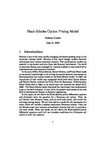
The Black and Scholes (1973) model is certainly one of the most used in …nance, but claims that this formula no longer holds in …nancial markets are also appearing with increasing frequency.1 In fact, there is a consensus nowadays to say that Black and Scholes ( 1973) model is somehow inconsistent with stylized facts. Empirical studies often report evidence of systematic errors between Black and Scholes theoretical prices and market prices. In particular, the model missprices out-of-the-money and in-the-money options.2 Moreover, when the Black-Scholes formula is inverted - although the volatility is a characteristic of the underlying asset return and consequently is not option speci…c - the implied volatilities estimates di¤er across exercise prices and maturities, and form patterns di¤erent from an horizontal line. Sometimes, the relation is a straight line with a negative slope and the pattern is called a “sneer”; sometimes, it is U-shaped and a “smile” or a “smirk” appears.3 This result is generally attributed to the unrealistic hypothesis of log-normality of the underlying asset return, combine with a constant volatility assumption. Indeed, if rare events are more frequent than it is supposed in the Gausssian case, then the price of in-the-money and out-of-the-money options will be higher than the Black and Scholes (1973) model predicts. The misspeci…cation of the distribution function tails leads, therefore, to more important implied volatilities for options whose strikes are far from the current price. Moreover, the density might not be symmetrical and, once more, this leads to di¤erent implied volatilities for options in-the-money or out-of-the-money: the implied volatility function may not be symmetric around the strike price. Under the assumption of nocorrelation between volatility and underlying asset return, Renault and Touzi (1996) have shown that Black and Scholes (1973) pricing formula overestimates at-the-money option prices and underestimates the others when considering a di¤usion model. To illustrate this phenomenon on the French market, we use the Black and Scholes (1973) model to compute the implied volatility of the French index CAC 40 call options quoted on the MONEP (Marché des Options Négociables de Paris) on the 14th, January 1997. The term to expiration of these options is March 1997. Figure 1 represents the implied volatility function on the y-axis whilst the moneyness is on the x-axis.4 - Please, insert Figure 1 somewhere here In order to avoid these drawbacks, di¤erent processes have been considered. For instance, a jump process had been chosen by Merton (1976) and more recently by Bates (1996-a and 1996-b), whilst Hull and White (1987), Stein and Stein (1991) and Heston (1993) considered stochastic volatility models. 1 See,

for instance, Rubinstein (1985 and 1994). Bates (1996-c) for a review. 3 Bates (2000) shows that smiles often appear before the crash of 1987 on the American market, whilst sneer patterns are more likely to be found since. ¢ ¡ 4 The moneyness is de…ned such as: M = [100 £ Ke¡r¿ ¡ S ¡r¿ ]: 0 =Ke 2 See

3

Bakshi et al. (1997 and 2000) develop a tractable option pricing model that admits stochastic volatility, stochastic interest rate and random jumps. But these approaches, which focus on …nding the “right” distribution, are still not perfectly satisfactory. Some of them are not parsimonious - that could lead to possible over…tting and to some estimation problems on not actively traded markets. Moreover, as shown by Das and Sundaram (1999), some of them lead to a volatility term structure di¤erent from the observed one. An alternative technique consists in using binomial or trinomial lattices that achieve an exact cross-sectional …t of option prices (see Rubinstein, 1994, Derman and Kani, 1994 and Dupire 1994). Nevertheless, the dimension of such models is still high and these approaches are based on the unrealistic hypothesis that the volatility is a deterministic function of asset price, maturity and moneyness. Possible over…tting and variability of the volatility function through time (see Dumas et al., 1998) seems to be the two major shortcomings of pricing with trees. Another approach, originally developped by Jarrow and Rudd (1982) and by Madan and Milne (1994), consists in approximating the density of returns with a normal or a log-normal one, corrected in some way. These methods would allow to improve the pricing and hedging performance by introducing supplementary parameters characterizing the skewness and the excess kurtosis of the underlying asset return densities. These models are, in some way, simpler since they do not require additional assumptions about risk aversion or correlation between volatility and underlying return for instance. Moreover, the number of parameter is quite small and, unlike stochastic or jump models, they depend only of the underlying asset return density function. Since, they seems more adapted to evaluation of density forecast; indeed, as Melick and Thomas (1997) write: “it is more natural to begin with an assumption about the future distribution of the underlying asset, rather than the stochastic process by which it evolves”.5 Moreover, several types of processes describe random variables that share the same density function (see Dupire, 1998). The purpose of this study is to check whether the approximation proposed by Jarrow and Rudd (1982) allows to improve the pricing of European CAC 40 index options traded on the French market.6 First, we evaluate in-sample pricing performance using several statistic and economic criteria. Second, we compare, separately, the impact of skewness and kurtosis departures from normality and evaluate the information contents of these variables in-sample and out-of-sample. Third, we compare continuous and discrete hedging performances of the models for a single asset hedging strategy portfolio. The paper is organized as follows. Section 2 is devoted to a short presentation of the Jarrow and Rudd (1982) model. Section 3 describes the French option market and the methodology. Section 4 presents the empirical results on pricing and hedging performances. Section 5 concludes. 5 For a survey of di¤erent methods of risk-neutral densities estimation methods, see, for instance, Cont (1997) and Jondeau and Rockinger (1998). 6 Only a few studies have been done in European stock market; see, for an example, Navatte and Villa (2000).

4

2

The Pricing of Options when Densities are Skewed and Leptokurtic

When option pricing is considered, the …rst element of interest is the conditional distribution of the terminal price of the underlying asset. The conditional distribution of the one-period change in the log-price of the asset is determined by the properties of xt+1 which can be de…ned as: xt+1 = ln St+1 ¡ ln St

(1)

where St is the price of the asset at time t. Over N periods, the change is:

ln ST = ln St +

N X

xj+1

(2)

j=1

¡ ¢ with T = t + N the expiration date. Then ST = St exp xN t+1 . The second element is the determination of the fair price in a risk-neutral framework. Indeed, a European call option is a contract which confers on its holder the right, with no obligation, to purchase an underlying asset, which current price is noted St ; for a prescribed amount, known as the exercise or strike price, denoted K, at the expiration date, T . Under the assumptions of complete market and no arbitrage opportunity, and if we suppose that the risk free rate of interest, denoted r, is constant, the theoretical price of a call option is the present value of the expected payo¤ at expirity: C (St ; K; ¿ ; rj£) = e¡r¿ EQ [M ax (ST ¡ K; 0)] Z +1 ¡r¿ = e (ST ¡ K) f (ST ) dST

(3)

ST =K

where EQ [:] is the expectation under the risk-neutral probability measure and £ is a vector of parameters characterizing the risk neutral density of the terminal spot process f (ST ). A close form for the option formula can then be obtained if we assumed a lognormal distribution for the terminal price of the asset, as in Black and Scholes (1973), or if we use a statistical series expansion for the conditional density of the price of the asset, as in Jarrow and Rudd (1982) or for its return as in Madan and Milne (1994).

2.1

The Black and Scholes (1973) model

Black-Scholes (1973) model assumes that the dynamics of the underlying asset follows a geometric Brownian motion: dSt = ¹ St dt + ¾ St dWt

5

(4)

with ¹ is a constant, ¾ represents the instantaneous volatility and Wt is a standard Brownian motion. Since the markets are supposed to be complete, Harrison and Pliska (1981) have shown that there exists a risk-neutral transformation which leads to the following expression: dSt = r St dt + ¾ St dWtQ

(5)

where WtQ is a Brownian motion under the risk neutral probability measure. It follows from Itô’s lemma that f (ST ) can be written as a log-normal density: 8 h ³ ´ ¡ ¢ i2 9 ST > 1 2 < = log ¡ r ¡ ¾ ¿ > St 2 1 p exp ¡ f (ST ) = (6) > > 2 ¾2 ¿ St ¾ 2¼ ¿ : ;

so the price of a European call option under the Black-Scholes (1973) assumptions is equal to: ¡ p ¢ (7) C (St ; K; ¿ ; rj¾)BS = St N (d) ¡ Ke¡r¿ N d ¡ ¾ ¿ with:

d=

log (St =K e¡r¿ ) + ¾ 2 ¿ =2 p ¾ ¿

The main advantage of this model is that all parameters, except the volatility, are directly observable. However, empirical evidence against the hypothesis that returns are homoskedastic and normally distributed, and the existence of some anomalies on option markets reported in several studies (see for instance Rubinstein, 1994) lead to the development of option pricing models based upon alternative processes. Whilst Black-Scholes (1973) model supposes that the continuous underlying asset return is normally distributed, Jarrow and Rudd (1982) have proposed a method to price options when densities are skewed and leptokurtic. The Black-Scholes (1973) model is then, a special case of the Jarrow-Rudd (1982) model. The basic idea is to approximate the unknown real density function of the underlying asset return by using skewness and kurtosis parameters.

2.2

The Jarrow and Rudd (1982) model

Series expansion have been widely used for pricing option since the seminal paper of Jarrow and Rudd (1982). Amongst the most popular statistical series used in …nance, one can distinguish expansions based on a normal distribution, the socalled Gram-Charlier Type A series (Backus et al., 1997, Corrado and Su, 1997, Knigth and Satchell, 1997, Brown and Robinson, 1999), expansions based on Hermite polynomials (Madan and Milne, 1994, Abken et al. 1996, Jondeau and Rockinger, 1998, Ané, 1999, Coutant, 1999) and Generalized Edgeworth series expansion based on a lognormal distribution (Jarrow and Rudd, 1982, Corrado 6

and Su, 1996, Jondeau and Rockinger, 1998).7 The Gram-Charlier Type B series expansion, series expansion based on Laguerre or Jacobi polynomials could constitute other natural candidates. In their original approach, Jarrow and Rudd (1982) suggest to use a lognormal distribution to approximate the real density function of the price of an asset. Indeed, following these authors, we can denote F (ST ) and A (ST ), respectively, the “true” cumulative density function of the underlying asset price and the approximating one. One supposes here that dF (ST ) = dST = f (ST ) and dA (ST ) = dST = a (ST ) exist, as well as moments one to four. Under these hypotheses, the density of the underlying asset price can be written as a function of the arbitrary density a (ST ) and its cumulants i (:) ; i = [1; 2; 3; 4]; as follows (see Appendix 1): # " k2 + (k1 )2 d2 a (ST ) da (ST ) + f (ST ) = a (ST ) ¡ k1 dST 2! dST2 # " 3 k3 + 3k1 k2 + 3 (k1 ) d3 a (ST ) ¡ 3! dST3 " # k4 + 4k3 k1 + 3 (k2 )2 + 6 (k1 )2 k2 + (k1 )4 d4 a (ST ) + (8) 4! dST4 + " (ST ) with ki = [ i (F ) ¡ i (A)] ; 1 (:) = ¹1 (:) ; 2 (:) = ¹2 (:) ; 3 (:) = ¹3 (:) ; 2 4 (:) = ¹4 (:) ¡ 3¹2 (:) where ¹i ; i = [1; 2; 3; 4] are the centered moments of order i, and " (ST ) is a residual. Second, third, fourth and …fth terms in the right side of the equation (8) allow to adjust a (ST ) according to the gap between the mean, the variance, the skewness and the kurtosis of the empirical distribution function and that of the approximating density (each term being weighted by the …rst, second, third and fourth derivatives of the approximating density function).8 The last part of equation (8) - the residual " (ST ) - takes into account terms in the development based on higher orders cumulants. If we assume moreover, following Jarrow and Rudd (1982), that the approximating distribution a (ST ) is the lognormal distribution, L (ST ), with the two …rst centered moments equal to the “true” ones, i.e.: ³ 2 ´ 2 r¿ and e¾ ¿ ¡ 1 (9) 1 (F ) = 1 (A) = St e 2 (F ) = 2 (A) = [ 1 (A)] 7 The last expansion could have been also called a Generalized Gram-Charlier Series since the sequence of the terms which appear in expansion are determined by the successive derivatives of the asset return density and not by a sequence of terms of ascending order as in the traditional Edgeworth series. For a complete review of the property of statistical series expansion, see Johnson and Kotz, (1994, pp. 25-30) or Kendall and Stuart, (1977, pp. 166-171). 8 Remark that the cumulants of f (S ) are de…ned as coe¢cients of di a (S ) =dS i T T T (i!)¡1 wether or not f (ST ) ¸ 0 and that f (ST ) may display multimodality (see Kendall and Stuart, 1977, pp 168-171, Johnson et alii,1994, pp25-30). Despite these limitations, it is often possible to obtain useful approximate expression of a distribution with known moments.

7

then the value for a European call option, C (F ) ; written on a stock St with strike K is: C (F ) = C (A) ¡ e

¡ r¿

k3 3!

Z1

(ST ¡ K)

K

+e¡ r¿

k4 4!

Z1

(ST ¡ K)

K

d3 L (ST ) dST dST3

(10)

d4 L (ST ) dST + » (ST ) dST4

where k3 = 3 (F ) ¡ 3 (A) ; k4 = 4 (F ) ¡ 4 (A), C (A) is the price of a European call under the Black-Scholes (1973) hypotheses and » (ST ) is a residual. Moreover, for j = [2; 3; 4], as we can write the j-th partial derivative terms such as: Z1

(ST ¡ K)

dj L (ST )

K

dSTj

dST =

dj¡2 L (K)

(11)

dSTj¡2

then the call option price is …nally equal to: C (F ) = C (A) ¡ e¡r¿ k3

dL (K) d2 L (K) + e¡r¿ k4 + » (K) dST dST2

(12)

The second term of the equation (12) corrects the pricing error due to the asymmetry of the original distribution function, whilst the third allows to take into account the phenomenon of heavy tails and the fourth term is a residual depending on the strike price. This statistical series expansion could obviously be based on higher moments, but one can think that higher moments than the fourth one, if they exist, would bring no supplementary valuable information.

2.3

Jarrow and Rudd (1982) Revisited by Corrado and Su (1996)

Corrado and Su (1996) show that equation (12) can be rewritten, dropping the remainder term » (K), under the next form: ¸ e¡r¿ dL (K) 3 (F ) ¡ 3 (A) 3=2 C (F ) = C (A) ¡ (A) (13) 2 3=2 3! dST 2 (A) ¸ e¡r¿ d2 L (K) 4 (F ) ¡ 4 (A) 2 + (A) 2 2 (A) 4! dST2 2 Recalling ³ 2 that ´ 3 (:) = ¹3 (:) ; 2 [St er¿ ] e¾ ¿ ¡ 1 , we have:

4

2

(:) = ¹4 (:)¡3¹2 (:) and

C (F ) = C (A) + ¸1 Q3 + ¸2 Q4 8

2

(F ) =

2

(A) =

(14)

with: ½

¸1 = ° 1 (F ) ¡ ° 1 (A) ¸2 = ° 2 (F ) ¡ ° 2 (A)

and 8 ³ ´3=2 ¡r¿ p > L(K) e < Q3 = ¡ (St er¿ )3 e¾2 ¿ ¡ 1 p 3! (d ¡ 2 ¾ ¿ ) K ¾ ¿ ³ 2 ´2 ¡r¿ ¡ ¢ p > : Q4 = (St er¿ )4 e¾ ¿ ¡ 1 e d2 ¡ 1 ¡ 5 ¾ ¿ + 6 ¾ 2 ¿ KL(K) 2 ¾2 ¿ 4!

where d is de…ned as in (7), ° 1 (:) and ° 2 (:) are the Fisher parameters for skewness and kurtosis: ° 1 (:) =

¹3 (:) 3=2 ¹2

(:)

and ° 2 (:) =

¹4 (:) ¡3 ¹22 (:)

and ¹i (:) the centered moment of order i, i = [2; 3; 4]. In the case of the lognormal density, Fisher parameters are equal to: 8 ³ ´1 ³ ´3 > < ° (A) = 3 e¾2 ¿ ¡ 1 2 + e¾2 ¿ ¡ 1 2 1 ³ ´ ³ ´2 ³ ´3 ³ ´4 > : ° 2 (A) = 16 e¾2 ¿ ¡ 1 + 15 e¾2 ¿ ¡ 1 + 6 e¾2 ¿ ¡ 1 + e¾2 ¿ ¡ 1 (15)

Parameters ¸1 and ¸2 measure, respectively, the excess skewness and the excess of excess kurtosis of the true density, and characterize the gap between the distribution function of the underlying asset price and the log-normal one. Parameters Q3 and Q4 , represent the sensitivities of the price of a speci…c option to departures from lognormality. The di¤erence between Black-Scholes and Jarrow-Rudd induced option prices is then a non-linear function of the excess moments, the level of the volatility of the market and the speci…c exercise price of the option considered. We illustrate the sensitivities of the option price to the excess moments in the Figure 2, which represents the value of ¡Q3 and Q4 parameters as a function of the moneyness of the speci…c option under valuation. They are the results of a simulation using the Corrado and Su (1996) formula with St = 100, ¾ = 0:15, r = 0:05, ¿ = 0:25; and K varying between 75 and 125. - Please, insert Figure 2 somewhere here Given (14), it is also possible to express analytically the implied volatility

9

(ISD) as (see Appendix 2): ¸ p ° (F ) ¡ ° 1 (A) = ¾ ¿+ 1 (St er¿ )2 (16) 3! ¸ ³ 2 ´3=2 ¡ p ¢ L (K) p £ e¾ ¿ ¡ 1 2¾ ¿ ¡ d K ¾ ¿ n (d) ¸ ° 2 (F ) ¡ ° 2 (A) 3 (St er¿ ) + 4! ¸ ³ 2 ´2 ¡ ¢ p L (K) £ e¾ ¿ ¡ 1 d2 ¡ 1 ¡ 5 ¾ ¿ + 6 ¾ 2 ¿ K 2 ¾ 2 ¿ n (d) p where ISD is the implied volatility that corresponds to the value of ¾ ¿ that equates the value of the Black-Scholes formula (1973) with the observed prices in the market, given values of other parameters …xed. It is clear from this formula that the implied volatility is a function of both skewness and kurtosis of the underlying asset return. Jarrow and Rudd (1982) show that their formula constitutes a good approximation of the option price when the underlying asset follows a Brownian process with jumps. Moreover, Jarrow and Rudd (1983) and Corrado and Su (1996, 1997) con…rm that the use of third and fourth moments seems to improve the pricing of European options. The aim of the next sections is to provide an empirical study of such a model applied on the French market. ISD

3

Database and Methodology

To evaluate the accuracy of the Jarrow-Rudd (1982) approximation, we apply their formula to the pricing of CAC 40 index call options traded at the MONEP. We then compare our results to those obtained following Black-Scholes methodology. The empirical study is led in two steps. In a …rst step, reversing the Black-Scholes and Jarrow-Rudd formulae, we estimate implied parameters (i.e. the second, the third, and the fourth moments) from options negotiated on the MONEP. Then, we use these information as input to evaluate the theoretical option prices, either in the Black-Scholes (1973) model or in the Jarrow-Rudd (1982) one and we compare those theoretical prices to market prices. This allows us to judge the in-sample performance of the di¤erent models. In a second step, we study the out-of-sample performance of each method.

3.1

The French Option Market

Option series used in this studies are extracted from the Bourse de Paris database from January 1997 to December 1998. The database includes a timestamped record of every trade occurred on the MONEP as well as dividends relative to underlying assets and transaction volume for all call and put options. It contains also the CAC 40 index caught every 30 seconds. Our study

10

focuses on long term European CAC 40 index call options (PXL contracts) traded at the MONEP in 1997 and 1998. The French CAC 40 index is composed of 40 French stocks listed on the monthly settlement stock market and selected in accordance with several requirements (such as capitalization or liquidity). The index is computed in realtime by taking the arithmetic average of quotations of assets that compose it, weighted by their capitalization (base value: 1,000 on 31 December 1987); it is disseminated every 30 seconds by the Bourse de Paris. The CAC 40 index and the daily returns associated are represented on Figures 3 and 4 on the whole sample. - Please, insert Figures 3 and 4 somewhere here -. Options written on CAC 40 index are the most actively traded of the MONEP on the sample period. In 1997 and 1998, an average of 745,309 option contracts were traded monthly and 35,775 daily. Premia reached, in average, FRF 4,8 billions a month and FRF 232 millions a day. Over these years, both equity and index options accounted for a roughly similar proportion of lots traded, but if we focus on transaction volume, equity options represented only 25% of the total amount corresponding to the sum of premia:9 Amongst the several contracts proposed on the French stock index, we focus on “Long term CAC 40 index options”. They are European-style, and correspond to two annual expiration dates: March and September (for two year period contracts). Two consecutive strike prices are separated by a standardized interval of 150 index points. For each option series (calls and puts), at all times, at least three strike prices are quoted: one at-the-money and two outof-the-money prices closest to the index value. During our sample period, the contract size is FRF 50, times the CAC 40 index; the minimum price ‡uctuation - the tick size - is equal to FRF 0.10 per index point, equivalent to FRF 5 per contract, and the cash settlement is equal to 50 times the di¤erence between the exercise price and the expiration settlement index.10 In-the-money options are exercised automatically at expiration, unless speci…ed otherwise by the buyer. Trading on this type of options started in 1991 and occurs since from 10:00 to 17:00. To avoid opening and closing e¤ect, we consider - as usual - only transactions that take place between 10:30 and 16:30. The choice of index options is essentially justi…ed by the fact that these options are the most actively traded and because returns on an index should be better …tted by a lognormal density than speci…c returns (Rubinstein, 1994). Nevertheless, as reported in Table 1, Jarque-Bera and Kolmogorov-Smirnov tests allow us to reject normality. Asymmetry and fat tails, as it has been documented several times for high frequency real time …nancial data (see for instance Maillet and Michel, 1998), are present in the index series. As shown in Table 1, such characteristics are veri…ed for high frequencies (hourly and daily 9 Further

informations are available on www.monep.fr. occured since the shift to the Euro.

1 0 Changes

11

returns). Moreover departures from normality - which is a key issue in this paper - is less strong when the frequency of observation is lower. - Please, insert Table 1 somewhere here -. The PIBOR 3 months, which was the most liquid maturity on the French market, serves as a proxy for the riskless rate of interest and is obtained from Datastream T M .11 As Harvey and Whaley (1992) shown, we have to adjust the index for discrete dividends. For each option contract, we calculate the present value of the future dividends paid on the index before the term to expiration of the option, noted D (t), such as: D (t) ´

¿ ¡t X e¡r(t;s)s D (t + s)

(17)

s=1

where r (t; s) is the risk-free rate for a bound of maturity s; s = [1; :::; ¿ ¡ t]: Dividends are also extracted from Bourse de Paris database. Because of liquidity problems, we used exclusion criteria to remove uninformative options record from the database. Those …lter rules are the following: options whose price is lower than 5 FRF, whose maturity is lower than 10 days or higher than 100 days are excluded from the sample.12 Moreover, a small number of market prices were deleted of the database because of arbitrage lower bound violations (70 out of the 12,500 options in the data had a negative time-value). On the sample, more than 12,500 prices are reported. In table 2, we classify options into nine sub-classes according to their maturities and their moneyness. By convention, a call option is said to be out-of-the-money (OTM) if its moneyness is lower than 0.96, in-the-money (ITM) if its moneyness is higher than 1.94 and at-the-money (ATM) otherwise; an option is said to be short-term if it has less than 40 days to expiration, medium-term if it has between 40 and 70 days to expiration and long-term otherwise. - Please, insert Table 2 somewhere here Table 2 shows the number of trade and trading volume across option moneyness and maturity category. Sub-classes are quite homogenous in term of 1 1 We have prefered to use the market riskless interest rate and the price index value series instead of the true value of implicit parameters obtained using Shimko’s method (see Shimko, 1993) - even if they are only proxies - to avoid problems linked to a related put database construction, the market perfectness assumption, the choice of the estimation method of CallPut parity relation, and …nally the choice of an outliers elimination method (see Venutelo and Péllieux (1997)). An alternative method, based on the absence of arbitrage opportunity (see, for example, Bakshi et al., 1997), should have required the Future CAC 40 index series which is not available, to our knowledge, on the whole periode of test used in this paper. 1 2 Most of the results obtained in this paper have been reproduced on a sample containing longer maturities. To save space and because of the lack of liquidity on such maturities, they are not printed here but are available on request.

12

representativeness: 45% of option prices are out-of-the-money, 35% are nearly at-the-money and 15% are in-the-money, whilst 35% of the option prices have a maturity lower than 40 days, 40 % have a maturity between 40 and 70 days, and 40 % have maturity higher than 70 days. The smallest number of options in a sub-class is equal to 705 (options in-the-money for long maturity). - Please, insert Table 3 somewhere here We also checked for anomalies regarding the liquidity of the French market on the sample. No speci…c problem was found in the sample, except for some dates where very few transactions took place. To avoid convergence problems in minimization algorithms (see next sub-section), we grouped observations belonging to successive business days in order to have a minimum of 25 transaction prices per date considered. Figure 5 represents daily transaction volumes for Long term CAC 40 call options in the sample, corresponding most of the time to business days or sometimes to grouped business days.13 - Please, insert Figure 5 somewhere here -

3.2

The Estimation Procedure

The theoretical price of an option contract depends on four observable parameters, the strike price, the maturity - both speci…ed in the contracts -, the underlying price, and the risk free interest rate - which can be taken from public market data - as well as some non-observable parameters describing the risk-neutral density function. One parameter is required in the Black-Scholes model - the volatility - and three in the case of Jarrow-Rudd one - the volatility, the skewness and the kurtosis. In implementing each model, we use all call options available on each given day, regardless of moneyness, as inputs to estimate implied parameters.14 We use a non linear least squared procedure in both cases where n is the number of all call options j; j = [1; :::; n]; available on a given day t, for a given maturity ¿ .15 The Black-Scholes optimal call price is de…ned such as CtBS = CtBS (b ¾ ¤t ) ¤ where ¾ bt should be the solution of the following minimization problem: 8 2 39 n < = X £ ¤ 2 ¾ b¤t = Arg M in 4 Cjobs ¡ C;jBS (b (18) ¾t ) 5 : ¾b t ; j=1

1 3 Only

13 % of business days were grouped - see Group 2 in Table 3. the widespread use of option-implied volatilities, there is no general agreement regarding weighting scheme (see Bates, 1996-c, for a review). We adopt the simplest strategy using the same weight for all options, since, anyway, our main goal is to provide equal chance to both models. Moreover, Corrado and Miller (1996) shown that simultaneous equations estimators and weighted average estimators have the same attainable variance lower bound, and, therefore, are equally e¢cient when used with appropriate weights. 1 5 We use the Broyden, Fletcher, Goldfarb and Shanno (BFGS) optimization algorithm. 1 4 Despite

13

³ ´ b ¤t b ¤t , where £ Similarly, the Jarrow-Rudd optimal call price, CtJR = CtJR £ is de…ned as the solution of the next minimization problem: 8 39 2 n h < ii2 = h X b1t Q b2t Q b 3t ¡ ¸ b 4t 5 b ¤t = Arg M in 4 ¾t ) ¡ ¸ £ (19) Cjobs ¡ CjBS (b : £ ; bt j=1

³ ´ b1t ; ¸ b2t the vector of the estimated parameters of ¾ t ; ¸1t and bt = ¾ with £ bt ; ¸ ¸2t . Fisher coe¢cients of the true distribution are given by: ( b1t + ° ° b1t (Ft ) = ¸ b1t (At ) (20) b ° b2t (Ft ) = ¸2t + ° b2t (At ) + 3

where ° b1t (At ) and ° b1t (At ) are estimated according to equation (15).16 In backing out implied parameters from all option prices on a day, we allow parameters to vary from day to day, which is inconsistent with the models assumption if parameters proved to be truly variable. Therefore, this procedure su¤er from a main, but usual, shortcoming. However, as noted by Renault (1997), even though there are no theoretical foundation for such a practice, it provides a quick and relatively accurate pricing strategy. Moreover, most empirical studies use this procedure (see, for instance, Bakshi et al., 1997 and Dumas et al., 1998).17 Because implied parameters have be found to be variable through time, we have preferred to consider all days in the sample instead of considering only some days spaced regularly in the sample. Thus, we have chosen to run the previous optimizations on non-overlapping periods which correspond to each business day - or grouped business days because of illiquidity problems (see previous section) - from January 1997, the 1st through December 1999, the 31th . Figure 6 illustrates the evolution of implied parameters back out from both models for options quoted between July 1997 to September 1997. After all the exclusions, the minimization algorithms converge for both models in all cases. - Please, insert Figure 6 somewhere here From …gure 6, we can notice that volatilities obtained with the two models are relatively similar (varying between 17% and 30 % with a correlation coe¢cient equal to 0.8951). We remark also that these parameter variations are not 1 6 The objective function in equations (18) and (19) would have been de…ned as the sum of squared percentage pricing error, and that would lead to assign more weight to relative cheaper options (i.e. out-of-the money and short term options). In the present case, we weight favourably relative expensive options (i.e. in-the money and long term options). Nevertheless, because the comparison between models will be based on several criteria (absolute and relative), this is not a key point (see next section). 1 7 Recently a singular approach was proposed by Bakshi et al. (2000). Indeed, in a stochastic volatility with jumps context, in which structural parameters have to be estimated, they use the method of simulated moment (MSM) to avoid this internal inconsistency.

14

so erratic whatever the model used. On the contrary, the path of the skewness is quite di¤erent according to the model chosen. Not surprisingly, on the whole sample, the implied distribution seems to be - as the density of the underlying asset- asymmetric since the skewness is negative in general. The path of the kurtosis is also quite di¤erent according to the model chosen. On the whole sample, the implied distribution seems to be - as the true one - leptokurtic since the kurtosis is higher than three in general. Moreover, those parameters seems to exhibit a strong autoregressive character as reported in Table 4. We check the sensitivity of parameter estimations in two ways. First, we performed a weighted non linear least squares estimation using as weights, the pricing errors of the equally weighted non linear least squares estimation ran previously. Second, we test the robustness of our estimations by excluding options one by one from our sample and repeating the estimation procedure for each sub-sample. This cross-validation procedure allows to control for possible measurement errors in the prices. Table 4 reports the mean, the standard deviation and the …rst autocorrelations for each implied parameters obtained with the various procedures. No obvious di¤erence can be hightlighted: implied parameters are very close whatever the weights scheme used. Di¤erences between the three procedures are always lower than the standard deviation of the estimation. Moreover, none of those methods provides lower standard deviations for all implied parameters. Estimations obtained with the three methods are …nally highly correlated. Accordingly, we will use only the …rst computation of the implied parameters in the following sections. - Please, Table 4 somewhere here The cross-correlations between implied moments estimated with the …rst method, for each models, are reported in Table 5 below.18 The implied volatility of the Benchmark model (BS) is highly correlated with the implied volatility obtained with other models. Moreover, the four implied volatilities are highly correlated one to another, whilst their are poorly correlated with higher implied moments in JR, JR Sk. and JR Kt. One can notice also that the parameters corresponding to the restricted models (JR Sk. and JR Kt.) are correlated with those of the complete model (JR). Finally, variations of implied skewness and kurtosis obtained with the two restricted models are quite independent of each other. - Please, Table 5 somewhere here According to these results, we can write that implied parameter estimations do not exhibit major anomalies on the sample whatever pricing models and methods. We can turn to the next section which is devoted to the pricing and hedging performances. 1 8 The implied moments cross-correlations corresponding to the two other methods (WNLS and average NLS, see table 3) are indistinguisable from those presented in Table 4.

15

4

Empirical Results on European CAC 40 Index Options

We …rst study the internal consistency of the implied parameters of the BlackScholes (1973) and the Jarrow-Rudd (1982) models. In the next sub-sections, we present in-sample and out-of-sample pricing performances. Then we turn, in the last sub-section, to measure the improvement obtained when pricing models are applied to hedging strategies.

4.1

The Alternative Models Pricing Performances

To state the comparison, we computed several criteria (see Appendix 3 for de…nitions): the Mean Error (FRF) which indicates the mean overpricing (if positive) or underpricing of model; the Mean Absolute Error (FRF) gives an idea of the size of the errors; the Mean Absolute Percentage Error, which represents the size of the errors expressed as a percentage of the price of the options; the Root Mean Square Error (FRF), which is the objective criterion considered in the optimizations; the Standard Deviation of Error (FRF) which indicates the variability of the error (expressed here in FRF); the Percentage of Positive Error for indicating a potential bias in the frequency of overpricing; the Overestimation (5% threshold) frequency of the model, which represents the frequency of large overestimation (over 5%); the Underestimation (5% threshold) which represents the frequency of large underestimation (over 5%). As pointed by Leitch and Tanner (1991) and Satchell and Timmerman (1995), statistical properties of models are not the only one to consider when comparing them. Their relative value - corresponding to economic agents - are also important. That is the reason why we also used the following economic criteria for the comparison: the Cumulative Linex Error, the Mean Logarithmic Error (FRF) and the Mean Mixed Error for Underestimations and for Overestimation. Thus, following Hwang et al. (1998 and 1999), we compared models using an asymmetric loss function. We advocated the use of Linex loss function de…ned as: £ ¡ ¢¤ ¡ ¢ Linex (Cn¤ ) = exp ¡a Cn¤ ¡ Cnobs + a Cn¤ ¡ Cnobs ¡ 1 (21)

where Cn¤ is the theoretical price, Cnobs the market price at time n and a an arbitrary coe¢cient function of the sensitivity of the representative agent to pricing error. Indeed, with an appropriate Linex parameter, we can re‡ect small (large) losses for underestimation or overestimation. In particular, a positive a will re‡ect small losses for overestimations comparatively to large losses for underestimations. An example of such function is given on Figure 15 (in Appendix 3) corresponding to Black-Scholes model.19 The comparison between 1 9 Due to the high number of observations in the sample, Linex functions corresponding to Black-Scholes and Jarrow-Rudd models are hardly distinguisable on a graph (see Figures 15 et 16).

16

models will be based on the Cumulative Linex criterion such as: CLinex (Ct¤ ) =

N X £ £ ¡ ¢¤ ¡ ¢ ¤ exp ¡a Cn¤ ¡ Cnobs + a Cn¤ ¡ Cnobs ¡ 1

(22)

n=1

The second economic criterion - Mean Logarithmic Error - results in a logarithmic transformation of the error terms assuming a logarithmic utility function of the economic agent. As in Brailsford and Fa¤ (1996), the comparison of models also relies on third and fourth criteria - the Mean Mixed Error (Underestimation) - which overweights the underestimation errors adopting the seller’s point of view who prefers to sell at an higher price than the market price, and the Mean Mixed Error (Overestimation) which, symmetrically, overweights the overestimation errors, adopting the buyer’s point of view who prefers to buy at a lower price than the market price (see Appendix 3 for de…nitions). Those two last criteria give another insight on economic value of models, focusing on behaviors of option market operators. 4.1.1

In-sample performance

In Table 6 are reproduced the several criteria (colon 1) we used to compare the Black-Scholes model (colon 2), the Jarrow-Rudd model (colon 3), the JarrowRudd model with the skewness adjustment but without the kurtosis adjustment (colon 4), and, the Jarrow-Rudd model with the kurtosis adjustment but without the skewness adjustment (colon 5). The comparison between Black-Scholes and Jarrow-Rudd leads in general to the conclusion of a better …t of the second model. Indeed, the Black-Scholes mean absolute error is equal to FRF 5.27 (which represents a mean relative error of 9.57% when considering option prices) to be compared with 2.21 (3.31%) in Jarrow-Rudd case. Furthermore, all models have a slight tendency to underprice options since the mean error is negative for all of them, but this mean underpricing is lower in the Jarrow-Rudd case. The root mean squared error and the standard deviation of the error are also drastically reduced for the Jarrow-Rudd model in-sample. Moreover, we note that, whilst the Black-Scholes formula goes with large overpricing at a large frequency (more than the third of the error sample - 37.61% - corresponds to large positive error), the Jarrow-Rudd model gives better results: the percentage of positive error is approximately equal to 50% and the frequency of large errors (positive or negative) are similar and equal to 9.3% or so. Figure 7, which represents an non parametric estimation of the density of the in-sample errors con…rms those results. Moreover, whatever the point of view adopted, a seller or a buyer of options would prefer the Jarrow-Rudd model since the mean logarithm error, the mean mixed errors for overpricing and for underpricing are far lower with this model. The use of cumulative linex error criterion would lead, in our case, to the same conclusion. - Please, insert Table 6 somewhere here - Please, insert Figure 7 somewhere here 17

It is also interesting to note - when we compare colons 2 to 5 of Table 6 that both skewness and kurtosis lead to improve the accuracy and the economic value of the pricing and that the skewness adjustment gives better results than the kurtosis adjustment. Finally, from …gures 8 to 11, which represent the error term as a function of the moneyness, one can notice that the moneyness bias is apparently diminished with Jarrow-Rudd (1982) model. - Please, insert Figures 8 to 11 somewhere here From Table 7, which reports the previous criteria according to the moneyness and maturity of speci…c options, the Black-Scholes (1973) model seems not adapted to price in-the-money and out-of-the-money options (even if deep in- and deep out-of-the-money options seem to be correctly priced). The di¤erence between models are the strongest in relative (absolute) terms when OTM (ITM) options are considered whilst distinguishing options according to their moneyness seems to be less relevant when Jarrow-Rudd model is estimated. - Please, insert Table 7 somewhere here On the contrary, the e¤ect of time to maturity are less evident. One could have expected to …nd a greater di¤erence between models when maturities are long, because departures from normality are more important when the frequency of observations is high. But, as in Backus et al. (1997), such relation is not valid on our sample since no general ranking can be found when di¤erent criteria are used. - Please, insert Table 8 somewhere here Improvements obtained are quite not surprising since we have supplementary degrees of freedom to improve the goodness-of-…t. Information criteria, such as Akaïke Information Criterion (AIC), Corrected Akaïke Information Criterion (AICc), Bayesian Information Criterion (BIC), or Schwartz Information Criterion (SIC), based on in-sample performances are reported in table 8. Those are calculated to examine the possibility of over…tting as they penalize the presence of more parameters. On the basis of those criteria, Jarrow-Rudd (1982) model dominates Black-Scholes (1973) one. Moreover, accordingly to the results reported in Table 8, when we compare the e¤ect of neglecting the impact of the excess of excess kurtosis, and the e¤ect of neglecting the impact of the excess of skewness on the option price, we can remark that the skewness gives more information about the market price and leads to a better improvement than the kurtosis when both considered separately. Nevertheless, taking into account both moments seems to lead to the best improvement and we cannot conclude that it is only due to a higher ‡exibility in the adjustment, adding two supplementary variables in the model. 18

A another way to test the bene…t of two additional variables could be found in considering out-of-sample performance of both models. The next sub-section consider such model performances using implied parameters backed out on the last business day and plugged into the theoretical formulae. 4.1.2

Out-of-sample performance

Considering the out-of-sample data, the accuracy and the economic value of Jarrow-Rudd model is higher since all statistic and economic criteria are reduced by far. The mean absolute error for the Black-Scholes model is now equal to FRF 6.21 (10.80%).20 One …rst notices that the results obtained with the BlackScholes (1973) model on the MONEP are not as accurate as those reported for the CBOE. To compare, the out-of-sample error obtained by Corrado and Su (1996) on the American market, is on average equal to USD 0.875 (4.3%).21 Their results are the same as those obtained by Bakshi et al. (1997) and Dumas et al. (1998) on the same market. As reported in Tables 9 and 10, this positive result holds whatever the moneyness and the maturity of options considered are. Figure 12, which represents the estimated out-of-sample error densities, indicates that the Jarrow-Rudd one is more centered around the mean, less asymmetric and has lower tails. We can remark also that Jarrow-Rudd out-ofsample error dominates the Black-Scholes one according to the second (and …rst) order dominance criterion since the probability of a smaller error (in absolute terms) is always higher in the Jarrow-Rudd model. - Please, insert Table 9 and Table 10 somewhere here - Please, insert Figure 12 somewhere here The three comparisons - in-, out-of-sample and based on information criteria - allow to conclude to the superiority of the Jarrow-Rudd (1982) model for all the selected criteria The pricing is then improved with this model. One question remains: is this improvement su¢cient to make a di¤erence when comparing models in term of hedging performances?

4.2

The Alternative Models Hedging Performances

Another way of judging the pertinence of an option pricing model is to compute the error corresponding to simple hedging strategies. The aim of this sub-section is to know whether Jarrow-Rudd (1982) model provide better risk management. 2 0 For some options, the error can be higher than 80%; however, the price of these options is generally very low. 2 1 Corrado and Su (1996) do not provide statistics about the relative error in their studies. The calculus we have done is the following: the relative error is equal to the absolute error from spread boundaries (0.64 USD on average), plus half of the bid-ask spread (0.47 USD), divided by the average price (20.22 USD) and multiplied by 100. For instance, the average error is equal to 4.3 % with a minimum of 3.2% and a maximum of 5.4%. The average error is computed such as: (0:64 + 0:47=2) ¤ 100=20:22 = 4:3%

19

Indeed, if the excess skewness and the excess of excess kurtosis of the true density give informations about the market price of options, setting hedge ratios based on the Jarrow-Rudd (1982) formula should present an improvement over the single volatility model. In this sub-section, we …rst give the delta and the gamma of a call option for the Black-Scholes (1973) model and the JarrowRudd (1982) one. In a second time, we use expressions of delta to compare the hedging performance of both models. This comparison is made in two steps. First, we test for continuous hedge, then, for discrete hedge. 4.2.1

The Greeks

Delta states the sensitivity of the option price to underlying asset price movements. By de…nition, it is the …rst partial derivative of the option price with respect to the underlying asset price. Gamma measures the sensitivity of deltahedged strategy payo¤ to the underlying asset price changes and is de…ned by the second partial derivative of the option price with respect to the underlying asset price. By computing …rst and second derivatives of the Jarrow-Rudd (1982) model for a European call option, we have the following expressions for the delta and the gamma: µ ¶ µ ¶ 3 4 @CtJR = N (d) + ¸1 Q3 + ¸2 Q4 (23) ¢JR = @ST ST ST and:

¡JR =

¡ p ¢¡1 @ 2 CtJR = n (d) St ¾ ¿ + ¸1 2 @ST

µ

6 ST2

¶

Q3 + ¸2

µ

12 ST2

¶

Q4

(24)

where N (:) and n (:) are, respectively, the cumulative density function and the density function of the standard Gaussian distribution, d is de…ned in equation (7) and ¸i ; Qj ; (i £ j) = [1; 2; 3; 4]2 correspond to equation (14). The …rst terms on the right-hand sides of equations (23) and (24) are the delta and the gamma of the Black-Scholes (1973) model whilst the second and third terms yield delta and gamma for Jarrow-Rudd models. 4.2.2

The Continuous and Discrete Hedging Strategies

In this section, we investigate the hedging performances of both models under evaluation. In fact, two aspects should be considered when judging the hedging performance: the pure model performance - viewed via the computation of the performance of a hedge portfolio continuously rebalanced through time and the improvement in risk management the model entails - which can be measured considering the results of a traditional self-…nanced single instrument strategy discretely rebalanced over the time. The latter takes into account realistic constraints (such as costs of strategies, discreteness of the series, tick size problem,...) whilst the former focuses only on the accuracy of the sensitivity 20

parameters of pricing formula.22 We then evaluate two types of ex post hedge portfolio errors: a continuous hedge portfolio error - denoted "0t+1 - and a discrete 00 hedge portfolio error - denoted "t+1 . In the continuous case, the replicating hedge portfolio (from one of the two option pricing models) is formed to replicate the value of an option at the next period. Following Dumas et al. (1998), we can de…ne the ex post continuous hedge portfolio error as: Z t+1 £ obs ¤ "0t+1 = Ct+1 ¡ Ctobs ¡ ¢ (Su ; u) dSu (25) u=t

where ¢ (:; :) is the sensitivity of the option price to in…nitesimal variations of the underlying asset price as reported in the last sub-section. It can be shown that to a large extent the hedging replication error re‡ects the di¤erence between the two periods. Indeed, if a model is correct to determine ¢ (Su ; u), and if the variation of the index price is the only relevant variable, a minimum requirement consists in the following equality: ¡ ¢ E "0t+1 = 0 (26)

and if we measure prices at di¤erent time t, the ex post continuous hedge portfolio error can be written as: ´ ³ ´i ³ £ obs ¤ h bt b t+1 ¡ Ct £ "0t+1 = Ct+1 (27) ¡ Ctobs ¡ Ct+1 £

b t is the set of parameter required in the computation of theoretical where £ prices. The aim of this comparison of continuous hedging performances is to assess whether although the Black-Scholes model exhibits pricing biases - as long as these biases remain relatively stable through time - its hedging performance can be better than the performance of a more complex model that can account for many of these biases, especially if the more complex model does not adequately characterize the way asset prices evolve over time. In order to compute a discrete hedge portfolio error, we build a traditional self-…nanced single instrument strategy based upon CAC 40 index contracts.23 To hedge the sell of a call option at time t, the investor has to be long in ¢t shares of the underlying asset and invest the residual (i.e. Ct ¡ ¢t St ) in a risk-free bond. Whilst the hedged portfolio is supposed to be riskless when there is an unique source of risk and when the hedging portfolio is rebalanced continuously, practical considerations - such as transaction costs or divisibility problems - lead some authors to evaluate discrete-time hedging performance where adjustments are made at discrete intervals. We suppose hereafter that the portfolio is rebalanced every business days. Then, the ex post hedging error, 00 at time t + 1, denoted "t+1 , is calculated as follows: 00

"t+1 = ¢t St+1 + [Ct ¡ ¢t St ] ert ¡ Ct+1 2 2 See

2 3 For

Dumas et al. (1998). examples of perfect delta-neutral hedges, see Bakshi et al. (1997).

21

(28)

where rt is equal to the risk-free rate for the business day t. This calculation is repeated for every t and for all options in the sample. 4.2.3

The Comparison of models in term of hedging performances

When we …rst compute the improvement in continuous hedging performance considering Jarrow-Rudd model, we have: :0

0

0

"t+1 = "JR;t+1 ¡ "BS;t+1 0

(29)

0

where "JR;t+1 and "BS;t+1 are the continuous hedging errors for Black-Scholes and Jarrow-Rudd models. ¡ BS ¢ ¡ JR ¢ :0 "t+1 = Ct+1 ¡ CtBS ¡ Ct+1 ¡ CtJR (30) Taking the expectation of the last equation gives: ³:0 ´ ¡ BS ¢ ¡ ¢ JR E "t+1 = E Ct+1 ¡ Ct+1 ¡ E CtBS ¡ CtJR

(31)

³:0 ´ and the empirical counterpart of E "t+1 ; t = [1; :::; N ¡ 1] where N is the total number of observations, is: "N ¡1 # X¡ X¡ ¢ N¡1 ¢ 1 :0 BS JR BS JR "t+1 = Ci+1 ¡ Ci+1 ¡ Ci ¡ Ci (32) (N ¡ 1) i=1 i=1 h³ 0 ´ ³ 0 ´i 0 0 1 "JR;N ¡ "JR;1 ¡ "BS;N ¡ "BS;1 = (N ¡ 1) As pointed by Nandy and Wagonner (2000), the expected improvement in hedging is related to the di¤erence between hedging error di¤erences computed for two dates. It is then expected to be very small and the Table 11 - in which the several criteria for the comparison are reported - con…rms this intuition. All statistic and economic criteria values are indeed very close for both models whatever the criterion considered is. The graphs of continuous hedging error density are, in fact, indistinguishable. In that sense, the Jarrow-Rudd model fails to improve signi…cantly delta-neutral hedging strategy and Black-Scholes model remains a di¢cult benchmark to beat, using continuous hedging performance criterion. - Please, insert Table 11 somewhere here When we second compute the improvement in discrete hedging performance considering Jarrow-Rudd model, we get this time with previous notations: ¤ £ 00 00 : 00 ¡ ¢BS [St+1 ¡ St ert ] "t+1 = "JR;t+1 ¡ "BS;t+1 = ¢JR t t 22

(33)

Taking the expectation gives: ³ : 00 ´ ³ : ´ ³ ´ ³ : ´ E "t+1 = E ¢t E Set+1 ¡ Cov ¢t ; Set+1

(34)

:

¡ ¢tBS and Set+1 = St+1 ¡ St ert : with ¢t = ¢JR t The expected improvement in hedging depends on the product of expected di¤erence in deltas, weighted by the expected premium on the index, and the covariance between the di¤erences in delta and ex post premia. It is then interesting to evaluate those components. First, we can notice, that the overall improvement depends crucially on the …rst term since the term in covariance is very low (it is equal to -0.0036 on the sample). Moreover, as illustrated in Figure 13, which represents time series of deltas corresponding to both models for speci…c options24 , the di¤erences between the deltas are very small. Indeed, for the whole sample, the mean di¤erence between deltas is, in absolute term, equal to 0.0079 (2.05%) - varying from -0.004 to 0.11 - as illustrated in Figure 14. - Please, insert Figure 13 somewhere here - Please, insert Figure 14 somewhere here When taking into account skewness and kurtosis, hedging coe¢cients have not been found very di¤erent one to another. In other words, since the co: variance between ¢t and Set+1 is small, the hedging coe¢cient ¢JR is not, on t our data, enough sensitive to departures from normality for causing a major improvement in discrete hedging strategies as indicated in Table 12 hereafter. - Please, insert Table 12 somewhere here When focusing on discrete delta-hedge strategy performance and for BlackScholes (1973) model, the mean hedging error is equal to FRF -1.73 and the mean absolute hedging error is equal to FRF 6.58 when considering at-themoney call options (and, respectively, FRF -2.28 and FRF 7.58 for the whole sample). These statistics are similar to those reported in Ané (1999) on the CBOE market since mean hedging error is USD -0.0753 and mean absolute hedging error is USD 0.5 for medium term options. Results regarding discrete hedging performances obtained with Black-Scholes (1973) and Jarrow-Rudd (1982) models are very close whatever the moneyness and the maturity considered. Most of the criteria are roughly the same for both models. Nor the importance of improvement, neither the directional accuracy criteria allows to conclude to the dominance of the Jarrow-Rudd model: the Black-Scholes delta is corrected in a right direction when taking into account skewness and kurtosis in only 44 % of the observations on the whole sample. As the sensitivity of option prices is an increasing function of the strike price, the 2 4 With

maturity September 97 and strike price equal to, respectively, 2350, 2650 and 2800.

23

relative error committed for both models naturally increases with the moneyness and the maturity of the option considered, but we …nd that the di¤erence in hedging performance between the two models does not depend on these speci…c characteristics as reported in Table 12. This quite negative result strongly di¤ers from those of Ané (1999) who applied Madan and Milne (1994) model on CBOE market. This failure could have di¤erent explanations. The …rst one could be found in a non signi…cative improvement of the Jarrow-Rudd model. In other words, the accuracy of the Jarrow-Rudd model is unfortunately still not su¢cient for making a real di¤erence with the Black-Scholes model when it is used for hedging purposes, but this …rst hypothesis contradicts results reported in previous sections that shown an important di¤erence between models accuracy. Another explanation of this failure could merely rely on the implied parameters variability - which entails movements in deltas that are not linked with price variations25 .

5

Conclusion

Our results lead to the conclusion that the Jarrow-Rudd (1982) option pricing model can, at least partially, explain the “smile” phenomenon and is superior in term of pricing errors. Both statistical and economic values of this model are better on the French market than those relative to the Black-Scholes (1973) model. This is true in-sample - as expected - because of the addition of two supplementary parameters in the pricing formula which helps for …tting the data. It is also true out-of-the-sample. Nevertheless, it has also been shown that the di¤erence between deltas are not important enough to yield a signi…cant improvement when hedging is the key issue of the use of options. The BlackScholes (1973) model still remain a di¢cult benchmark to beat. These conclusions point us in a number of directions for future research. The …rst one is, following the approach of Hwang and Satchell (1998) or Rosenberg (2000), to focus on a dynamic approach of the comparison between models, using autoregressive forms of the three parameters dynamic considered in the Jarrow-Rudd (1982) option pricing model. Another concerns the use of di¤erent statistical series expansion. The use of Gamma distribution (Heston, 1993-b) or Beta distribution (Corrado,1999) as approximation of the true distribution constitute also interesting alternative approaches. A last direction would consist of a more general comparison of the hedging performances and the pricing accuracy of the di¤erent forms of four moment option pricing models. 2 5 As

³ : ´ et+1 in equation (34). hightlighted by the term Cov ¢t ; S

24

References

Abken P., D. Madan and S. Ramamurtie, (1996), “Estimation of RiskNeutral and Statistical Densities by Hermite Polynomial Approximation with an Application to Eurodollar Futures Options”, Working Paper, Federal Reserve Bank of Atlanta. Ané Th., (1999), “Pricing and Hedging S&P 500 Index Options with Hermite Polynomial Approximation: Empirical Tests of Madan and Milne’s Model”, Journal of Futures Markets 19 (7), 735-758. Backus D., S. Foresi, K. Li and L. Wu, (1997), “Accounting for Biases in Black-Scholes”, Working Paper, Stern School of Business, 40 pages. Bakshi G., Ch. Cao and Z. Chen, (1997), “Empirical Performance of Alternative Option Pricing Models”, Journal of Finance 52 (5), 2003-2049. Bakshi G., Ch. Cao and Z. Chen, (2000), “Pricing and Hedging Long-Term Options”, Journal of Econometrics 94, 277-318. Bates D., (1996-a), “Dollar Jump Fears, 1984:1992, Distributional Abnormalities Implicit in Currency Futures Options”, Journal of International Money and Finance 15 (1), 65-93. Bates D., (1996-b), “Jumps and Stochastic Volatility: Exchange Rate Process Implicit in Deutsche Mark Options”, Review of Financial Studies 9 (1), 69-107. Bates D., (1996-c), “Testing Option Pricing Models”, Handbook of Statistics 14: Statistical Methods in Finance, Maddala and Rao (Eds), 567-611. Bates D., (2000), “Post-’87 Crash Fears in the S&P 500 Futures Option Market”, Journal of Econometrics 94, 181-238. Black F. and M. Scholes, (1973), “The Pricing of Options and Corporate Liabilities”, Journal of Political Economy, 637-655. Brailsford T. and R. Fa¤, (1996), “An Evaluation of Volatility Forecasting Techniques”, Journal of Banking and Finance 20, 419-438. Brown C. and D. Robinson, (1999),“Option Pricing and Higher Moments”, Proceedings of the 10th annual Asia-Paci…c Research Symposium, February, 36 pages. Cont R., (1997), “Beyond Implied Volatility”, Econophysics, Kertesz and Kondor (Eds.), Amsterdam: Kluver. Corrado Ch., (1999),“General Purpose, Semi-Parametric Option Pricing Formulas”, Working paper of Department of Finance, University of Missouri-Columbia, 36 pages. Corrado Ch. and T. Miller, (1996), “E¢cient Option-Implied Volatility Estimators”, Journal of Futures Markets 16 (3), 247-272. Corrado Ch. and T. Su, (1996), “S&P 500 Index Option Tests of Jarrow and Rudd’s Approximate Option Valuation Formula”, Journal of Futures Markets 16 (6), 611-629. Corrado Ch. and T. Su, (1997), “Implied Volatility Skews and Stock Index Skewness and Kurtosis Implied by S&P 500 Index Option Prices”, Journal of Derivatives, summer. Coutant S., (1999), “Implied Risk Aversion in Options prices Using Hermite

25

polynomials”, Working paper of CEREG n ± 9908, University of Paris-Dauphine, 34 pages. Das S. and R. Sundaram, (1999), “Of Smiles and Smirks: A Term-Structure Perspective”, Journal of Financial and Quantitative Analysis 34 (2), 211-240. Derman E. and I. Kani, (1994), “Riding on a Smile”, Risk 7 (2), 32-39. Dumas B., J. Fleming and R. Whaley, (1998), “Implied Volatility Functions: Empirical Tests”, Journal of Finance 53 (6), 2059-2106. Dupire B., (1994), “Pricing with a Smile”, Risk 7 (1), 18-20. Dupire B., (1998), “Pricing and Hedging with Smiles”, Volatility New Estimation Techniques for Pricing Derivatives, R. Jarrow (Ed.), Risk Books. Harrison J. and S. Pliska, (1981), “Martingales and Stochastic Integrals in the Theory of Continuous Trading”, Stochastic Processes and their Applications 11, 215-260. Harvey C. and R. Whaley, (1992), “Dividends and S&P 100 Index Option Valuation”, Journal of Futures Markets 12 (2), 123-137. Heston S., (1993-a), “A Closed-Form Solution for Option with Stochastic Volatility with Applications to Bond and Currency Options”, Review of Financial Studies 6, 327-343. Heston S., (1993-b), “Invisible Parameters in Option Prices”, Journal of Finance 48 (3), 933-947. Hull J. and A. White, (1987), “The Pricing of Option with Stochastic Volatilities”, Journal of Finance 42, 281-300. Hwang S., J. Knight and S. Satchell, (1999), “Forecasting Volatility Using LINEX Loss Functions”, manuscript, Trinity College, University of Cambridge, 20 pages. Hwang S. and S. Satchell, (1998), “Implied Volatility Forecasting: A Comparison of Di¤erent Procedures Including Fractionally Integrated Models with Applications to UK Equity Options”, in Forecasting Volatility in the Financial Markets, Knight and Satchell Ed. (BH), 193-225. Jarrow R. and A. Rudd, (1982), “Approximate Option Valuation for Arbitrary Stochastic Processes”, Journal of Financial Economics 10, 347-369. Jarrow R. and A. Rudd, (1983), “Tests of an Approximate Option Valuation Formula”, in Option Pricing Theory and Applications, Brener (Ed.), Lexington MA: Lexington Books, 81-100. Jondeau E. and M. Rockinger, (1998), “Reading the Smile: The Message Conveyed by Methods which Infer Risk Neutral Density”, CEPR Discussion Paper 2009. Johnson N., S. Kotz and N. Balakrishnan, (1994), Continuous Univariate Distributions, Second Edition, Vol. 1, John Wiley, New-York. Kendall M. and A. Stuart, (1977), The Advanced Theory of Statistics, Fourth Edition, Vol. 1, Macmillan Publishing Company, New York. Knight J. and S. Satchell, (1997), “Pricing Derivatives Written on Assets with Arbitrary Skewness and Kurtosis”, manuscript, Trinity College, University of Cambridge. Leitch G. and J. Tanner, (1991), “Economic Forecast Evaluation: Pro…t versus the Conventional Error Measures”, American Economic Review 81 (3), 26

215-231. Madan D. and F. Milne, (1994), “Contingent Claims Valued and Hedged by Pricing and Investing in a Basis”, Mathematical Finance 4, 223-245. Maillet B. and Th. Michel, (1998), “Volume Time-scale and Intra-day Returns Density”, Proceedings of the Second International Conference on High Frequency Data in Finance, June, 24 pages. Melick W. and Ch. Thomas, (1997), “Recovering an Assets Implied PDF from Options Prices: An Application to Crude Oil during the Gulf Crisis”, Journal of Financial and Quantitative Analysis 32 (1), 91-116. Merton R., (1976), “Option Pricing when the Underlying Stock Returns are Discontinuous”, Journal of Financial Economics 4, 125-144. Nandy S. and D. Wagonner, (2000), “Issues in Hedging Options Positions”, Federal Reserve Bank of Atlanta Economic Review, First Quarter 2000, 24-39. Navatte P. and C. Villa, (2000), “Implied Skewness and Kurtosis: Smile E¤ect and Empirical Series Properties”, The European Financial Management Journal 6 (1), 41-56. Renault E., (1997), “Econometric Models of Option Pricing Errors, Advances in Economics and Econometrics: Theory and Applications 3, Kreps and Wallis (Eds), ESM, Cambridge University Press, 221-278. Renault E. and N. Touzi, (1996), “Option Hedging and Implied Volatilities in a Stochastic Volatility Model”, Mathematical Finance 6, 279-302. Rosenberg J., (2000), “Implied Volatility Functions: A Reprise”, Journal of Derivatives 51, Spring 2000, 51-64. Rubinstein M., (1985), “Non Parametric Tests of Alternative Option Pricing Models Using All Reported Trades and Quotes on the 30 Most Active CBOE Option Classes from August 23, 1976 through August 31, 1978”, Journal of Finance 40, 455-480. Rubinstein M., (1994), “Implied Binomial Trees”, Journal of Finance 49, 771-818. Sangupta J. and Y. Zheng, (1997),“Estimating Skewness Persistence in Market Returns”, Applied Financial Economics 7, 559-566: Satchell S. and A. Timmermann, (1995), “An Assessment of the Economic Value of Non-linear Foreign Exchange Rate Forecasts”, Journal of Forecasting 14, 477-497. Scott L., (1987), “Option Pricing When the Variance Changes Randomly: Theory, Estimators and Applications”, Journal of Financial and Quantitative Analysis 22, 419-438. Shimko D., (1993), “Bonds of Probability”, Risk, April, 33-37. Stein E. and J. Stein, (1991), “Stock Price Distributions with Stochastic Volatility”, Review of Financial Studies 4, 727-752. Venutolo T. and G. Péllieux, (1997), “Empirical Results from the GARCH Option Pricing Model”, Proceedings of the AEA-BNP-Imperial College Conference, June, 28 pages.

27

Appendix 1 The function F (ST ) is the “true” cumulative density function and A (ST ) will be the approximating one. We suppose that dF (ST ) =dST = f (ST ) and dA (ST ) =dST = a (ST ) exist, as well as the …rst N non central moments of the distribution function F . Formally, the …rst cumulants j (F ), j = [1; :::; N ¡ 1] ; are given by the following equality (see Kendall and Stuart, 1977, p.73): 3 2 N¡1 j X ¢ ¡ (it) 5 + o tN¡1 (A1) ln Á (F; t) = 4 j (F ) j! j=1

where Á (F; t) is the characteristic function of F and i2 = ¡1. Taking exponential and using the de…nition of the characteristic function of A, transforms the equation A1 into:

Á (F; t) = exp

8 ¡1 0] M M E (U ) = £ n n N n=1

U h¯ X ¯ ¯ ¯ ¯Cn¤ ¡ Cnobs ¯2 £ 1I[C ¤ ¡C obs 0] and U =

n=1

N P

n=1

1I[Cn¤ ¡Cnobs

(A15)

¤ ¡C obs 0] Cn n

# i

0] :

Mean Mixed Error (Overestimation) 2 O ¯ 1 4 X h¯¯ ¤ obs ¯2 M M E (O) = £ + Cn ¡ Cn £ 1I[Cn¤ ¡Cnobs >1] N n=1

U i X ¯ ¯1=2 ¯ ¤ ¯ ¯Cn ¡ Cnobs ¯ £ 1I[C ¤ ¡C obs + ¯Cn¤ ¡ Cnobs ¯ £ 1I[0