of plagioclase or a decrease in tbe grossular content of garnel, or both. Indeed, this is. Iypically the case in metamorphic rocks. Rocks crystallized at low pressure ...
Chapter 15
The calculation of metamorphic phase equilibria I: Geothermometry and geobarometry In earlier chapters we examined the types of metamorphic paragencses thai occur along diverse P~T paths for rocks of different bulk compositions. The purpose of doing these exercises was 10 get a feel for the types of mineral reactions that are to be expected along typical P-T trajectories. Of course, these are all hypothetical scenarios and the real work of the petrologist comes in trying to detennine the actual history in light of the bils of evidence found in the rock. In these previous discussions we concentrated mainly on the mineral assemblages without considering in any quantitative detail the compositions of the minerals along the P-T paths. However, mineral compositions can be very sensitive indicators of metamorphic P-T conditions and P-T paths so there is potentially a wealth of infonnation in the study of the evolution of mineral chemistry. GENERAL METHODS
To use mineral compositions effectively we will need to examine how to calculate metamorphic phase equilibria in systems that approach real rocks. All of the possible phase equilibria approaches are based on the conditions of equilibrium, which state that
For any stoichiometric relation of the fonn m
0= IUjMj
(15-1)
j=l
that can be written among components ofphases i1l a chemical system, an equivalent expression can also be written among the chemical potentials of those phase components: m
o = IUj~j
(15-2)
j:1
where M j is the chemical symbol of the jlh phase component, Uj is the stoichiometric coefficient of the jlh phase components in the reaction, and Ilj is the chemical potential of the jth phase component and the sununation is over all m phase components in the reaction. Equation 15-2 can be expanded to give an expression for the equilibrium constant (~) as a function of pressure and temperature:
Geothennometry and Geobarometry
512
t>G(P,T,X) = 0 = t>H(298,1) +
JT
P
t>CpdT +
2 8
-J 'l
t>5(298,1) +
Jt>V
dP
I
It>i
p
dT)+ RTlnIH(298,1) = Hc(298,1) + 4HD(298,1) - 2H A (298,1) - 3HB(298,1)
(15-5)
Geothermometry and Geobarometry
115(298.1) =5c(298.1) + 450(298.1) - 25 A (298.I) - 35,(298.1)
513 (15-6)
=Vc + 4Vo - 2VA- 3VB
(15-7)
6.Cp = C pc + 4C PD - 2CPA - 3CPB
(15-8)
6.V
where .6.H(298,1), .6.5(298,1)• .6.V and .6.Cp are called the enthalpy, entropy, volume and heat capacity of reaction, respectively. From Chapter 6 it will be remembered that Cp and V are functions ofT and P so that the integrals of .6.Cpand.6.V must be done explicitly (see Eqs. 6·62, 6-63 and 6-70). Typically the heat capacity integral T
( 15-9)
IIICpdT 248
is done at a pressure of I bar (because that is the pressure at which most heat capacities are determined) and the volume integral p
JIIV
(15-10)
dP
1
is done at the temperature of inleresl. Equivalent forms of Equation 15-3 may be written by performing the integrals to calculate.6.5 and.6.H of reaction at T and P. From Chapter 6 it will be remembered that the enthalpy and entropy al any temperature are calculated from the heat capacity integrations (see Eqs. 6-56 and 6-59): T
H(T. I) = H(298. 1) + ICpdT
(15-11)
248 T
j¥ dT
5(T. 1) = 5(298.1) +
(15-12)
298
Making these substitutions, Equation 15-3 may be wriuen p
IIG(P.T.X) = 0 = 6H(T.I) - T 65(T.I) + J 6V dP + RTInK. q
(15-13)
1
where.6.H and.6.$ are now computed at I bar and the temperature of interest (T in Kelvins). It is also JXIssible to make the explicit pressure correction: p
H(T. P) = H(T. 1) + f(V - VaT) dP
(15-14)
1
p
5(T. P) = 5(T.I) - fva dP 1
(15-15)
514
Geothennometry and Geobarometry
from which the equivalent expression for.6.0 of reaction may be written "O(P.T.X) = 0 = "H(T.P) • T "S(T.P) + RTln~
(15·16)
where now 6H and 6S are computed al the T and P of interest. In Chapter 7 the close relationship between activity and entropy of mixing was established. By regrouping tenns in Equation 15-13 we may write
,,0
=0 = "H(T.P.Xl . T : HokIaway and Lee(lm): Pm:hllkllld uvrtDt'evl (1981)
R.Ibcirn Ind -eell coexisllnalt1UlCOY1te Md pInpite
AlI~
(1986)
518 Net transfer
Geothennometry and Geobarometry ~ulllbri.
~nl (1976); Ghenl et aI. (1979); ~wton and Hasdtoll (1981): Hodp and Spell' (1981); Ganguly and SnCIII (19804): HodlO and Royden (1984); ~ll and Holland (1988); kor.iol and
Nttlo1Oll (1988): Koz.iol (1989)
Ghent and SlouI (1981): Hoo1ga: and Crowley (19&5); Hoitch (1991) Ghent and SIOUt(I98II: HodJU and Crowley (I98.S); Powell and Holland (1981)
3FcPiC4 -+ 3CaAl-2SiA s Ca}Al-zSiJ012 -+ lFqAhSiJOn
3FcSiOJ -+ 3CaAl}Si:zOs = ~ ·f'IoIiocu- .
c1mo,,)'routIt· qwDl'tl:
Wood (1975); Bohlen et aI. (198Ja.c)
Newton and Pmins (1981); Bohkn d al. (1983&); and Chipen. (I98S)
2FeJAhSi)On -+ CajAlPi)On -+ 3SiC;!
~
3CaM,si:z06 -+ 3CaAQSiA " 2CIo}A12Si)012 -+ MlJAl2Si]Oll -+ 3Si02
Newton and Pukint (198'2): Pnki/1ll (l987); Powell and Holl.nd (1988); Mocdla' d aI. (1988)
FeJAI;!Si)OI2 -+ 3Ti02" JFeTrOl + AI2Si~ -+ 2S~
Doblen tl ai, (198Jb)
Gamel ·pkJgioclost . cl~·quam:
GonwI·pklgioc~·l'Illik·
il_nilt-qlKJrf:t. (GRIPS)
GarMl·",tik·ilmm;/eAl2SiOS-qlUlrfl. (GRAIL)
Bohlen and Uon. (1986) Bohlen InC! Liotta (1986)
Ghent and SIOUI (l9S4)
Essene and Bohlen (19&5) Eu.ene and Bohlen (1985)
GDmrr
M.
When discussing element partitioning, it is common to define a term known as the distribution coefficient which is the equilibrium constant but without the exponent (3 in this case):
K_(X~~ X~) _ D=
xGrt XB1 Fe Mg
-
(MglFe)Gn (V)1I3 (MglFe)Bt = '--eq
(15-35)
T = 500·C
T = 800·C KD = 0.30
KD = 0.14
(a)
(b)
MgO
Biotite
Mg/(Fe+Mg) biol.e
••
'-0
Mg/(Fe+Mg) biotite
Figure 15·3. Plots showing the disposition of gamet-biotite tie lines al differenl temperatures on two different diagrams. (a) and (b) are AFM diagrams and (e) and (d) are ternary reci~a1 exchange diagrams. (a) and (e) are at a temperature of approximately 5OO·C where the partitJoning is greater. whereas (b) and (d) are at a lemperalUre of 8OO·C where the partitioning is smaller.
Geothermometry and Geobarometry
521
There are several different ways that element partitioning between two phases may
be displayed, as shown in Figures 15·3 and 15-4. For the minerals garnet and biotite, the element partitioning is revealed on the AFM diagram by the slope of the tie lines between these two minerals. At low temperature the slope is large and at high temperature the slope is more nearly radial from the A120) apex. Note that a line radiating from the A120) apex is a line of constant FelMg so any tie line parallel to such a line signifies no partitioning. A closely related diagram is the ternary reciprocal exchange diagram shown in Figure 15-x and d. This diagram is simply a squared off version of the composition plane that contains lhe two garnet and two biotite end members. Remember that the two solid solutions aJmandine·pyrope and annite-phlogopite must be parallel in composition space because they are both related by the same exchange vector (FeMg_I). Note also that in the limit of the pure Fe or pure Mg system, the tie-lines approach the vertical. Althougn the equilibrium constant is a constant over the entire diagram. in the end member KFASH or KMASH systems it becomes undefined because the exchange reaction can no longer be written. Figure 15-4 shows three other ways of displaying element partitioning data. Starting with Equation 15-35 and substituting On
XFe
=I • XGn Mg
Bl
Bl
and Xn = I - XMg
we arrive at
.."
1.0
c 0.8 ~ Cl 0; 0.6
--"
(0)
c
. '"
•+ 0.4
IL
'"
IL
.0 0.2 0.4 0.6 0.8
1.0
Mg/(Fe+Mg) Biotite
-E
.
1.0
9
"-
2.0
~ 1.0
0.2 00
(b) 4.0
Cl 3.0
::;
1£ ::;
5.0
00
1.
4.0 5.0
(Mg/Fe) Biotite
(e)
0.0
~
" -1.0
~ -2.0 ::; ,£-3.0 -4.0
-5.0-3.0 brotn"-:Tn'-,,--'-nH -2.0 -1.0 0 1.0 2.0
In(MglFe) Biotite
Figure 15·4. Three ways of showing the partitioning of Fe and Mg between two phases such as gamet and biotite. (a) is a plot of XMg :: Mg/(Mg+Fe) in each phase for different values of Ko. (b) and (e) are plots of (MglFe) and the natural logarithm of (Mg/Fe) in each phase. respectively. In (b) Ko is the slope and in (e) InKo is the intercept at In(MgIFe)Biol:i!e = O.
-------------------
522
Geofhennometry and Geobarometry
x·' X·,
Kc::M& (15-36)
A plot of x~~ versus X~11g is shown in Figure 15-4a. Again starting with Equation 15-29 onc can derive the relation
_ (~)., Fe -KD Fe (~)Gn
(15-37)
which is plotted in Figure 15-4b. Alternatively, we can take the log of Equation 15-37 and arrive at
as plotted in Figure 15-4c. The three plots in Figure 15-4 are functionally equivalent and any of the three may be used to infer the KD value of gamet-biotite pairs. For example, if a suite of gametbiotite analyses are plotted then from Figure 15-4a (Eq. 15-36) the KD can be inferred from the line along which the data plot. In Figure 15-4b (Eq. 15-37) the Ko is the slope of the line and in Figure lS-4c (Eq. 15-38) the InKo is the intercept on the plot. How well the data either CA) fall on onc of the curves in Figure 15-4a, (B) fall on a straight line in Figure 15-4B or (C) fall on a line with a slope of 1.0 in Figure 15-4c is a measure of the constancy of Ko for the sample set. Dissimilar Ko values will also show up on the plots in Figure 15-3 because the tie lines will not show consistent behavior and will sometimes even cross. Crossing tie lines is one good indication for lack of complete equilibration in a sample set. One important reason why Ko might not be constant is that the samples are not well equilibrated so plots such as these are used to test for equilibration in a sample set. However, another likely reason that Ko might not be constant is that the solid solutions involved (here garnet and biotite) are not ideal so that the activity models used are inadequate. If this is the case then there is typically a visible trend to the variation of Ko with composition. For instance, values of Ko in Mg-rich samples may be high whereas values of Ko in Fe-rich samples may be low. For many compositions of garnet and biotite there is no large deviation from ideal solution behavior so that plots such as Figure 15-3 and 15-4 can be used to evaluate the degree to which the samples are equilibrated. An experimental calibration of the partitioning of Fe and Mg between garnet and biotite was published by Ferry and Spear (1978). In these experiments, garnet of known composition was equilibrated with biotite of unknown composition at temperatures ranging from 550-8oo"C. After the experiment, the composition of the biotite was analyzed by electron microprobe and the Ko calculated at each experimental temperature. Because the experiment was run with a large amount of garnet and only a small amount of biotite, it could safely be assumed that the composition of garnet did not change during the experiment. The data were plotted on a plot of InK o versus Iff (Fig. 15-5) and a line regressed through the points:
Geotllermometry and Geobarometry
800 750
T re) 700 650
600
550
0
•
523
-2.0
-1.8 0
-1.6
"
-1.4
'"
-1.2
InKo
=-~ T(K)
+ 0.782
0
-1.0 '-----'-_-'---''--"-_.L---'_--'
9.0
10.0
11.0
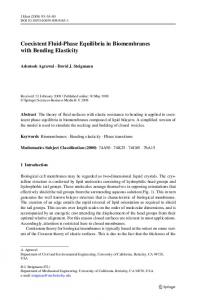
Figure 15-5. Plot of JoKo versus 1([ for experimentally equilibrated gamet-biotite pairs. P = 2.07 kbar. From FeI'T)' and Spear (1978).
12.0
10,OOOfT(K) -2109 InKo = T(K)
(15-39)
+ 0.782
This is an explicit relationship between loKo and temperature detennined from an experimental study. The formal thermodynamic relation was given in Equation 15-3 and comparison of Equations 15-39 and 15-3 permits evaluation of the thermodynamic properties of the reaction. To do Ihis, however, requires knowledge of the .1Cp and t! V of reaction. For many reactions a simplification can be made because even though C p is a strong function of T. the .1.Cp of reaction may be relatively small. Thai is, for many reactions the assumption .1Cp = 0
( 15-40)
is reasonable and Equalion 15-3 simplifies to p
0= 6H(29B, I) + 16VdP - T6S(29B,I) + RTlnK,q
(15-41)
A second simplification can often be made when the reaction studied involves only solid phases. The pressure and temperature dependence 01 the volume of a crystal is not large and the .6. V of reaction for a reaction that involves only solid phases is very nearly independent of P and T over the range of pressures and temperatures encountered in the crust. If it can be assumed that .6. V = constant, then it can be moved outside of the integral in Equation 15-10 to give p
p
J6V dP =6V J dP ="V (P -
1
I)
(15-42)
1
With this simplification, the pressure and temperature dependence of the equilibrium constant becomes 0= 6H(29B,I) + 6V (P - I) - T6S(29B,I) + RTlnK,q
(15-43)
Geothennometry and Geobaromerry
524
It must be remembered Ihal Equation 15-43 is only valid for reactions in which 6Cp = 0 and 6 V = constant. Therefore, it is not valid for a dehydration reaction in which the volume of one of the participating phases (H20) is a strong function of P and T. For the gamet-biotite Fe-Mg exchange reaction the above assumptions are quite
reasonable. For example. if tJ.C p were not equal to zero, then the data in Figure 15-5 would plol as a curve. Inasmuch as no curvature is apparent, the assumption 6Cp
=0 is
reasonable. Comparing Equations 15-39 and 15-43 we have 65(298,1) = 3 R (0.782) = 19.51 J/mle-K AH(298,1) = 3 R (2109) - (2070 - l) ban; AV
=52,112 j/mole
where 2070 bars is the pressure of the experiments and a vaJue of IiV = 0.238 Jlbar (2.38 em) has been adopted from molar volume measurements on end member minerals. The factor 3 enlers in because Equation 15-43 is written in terms of Kcq whereas Equation 15-39 is written in tenus of Ko (see also Eq. 15-35). The full equation is therefore 52.112 - 19.51 T(K)
+ 0.238 P(bars) + 3RTInKo = 0
(15-44)
Figure 15-6 is a plot of Equation 15-44 where values of Ko have been contoured on a P-T diagram. The slope of these lines is fairly steep: dP _ (AS - 3RlnKD) _ (19.51 - 3RlnK D) AV 0.238 dT -
=
which varies from 323 bars/degree for Ko = 0.1 to 208 bars/degree for Ko 0.3. Therefore. the geothermometer is relatively insensitive to the assumed pressure of equilibration.
14
12 10
o
~
o
"
~ c...
6 4
2
Ky'
Sil
And
oL...,4:-=070---'---;5:-=070---'--6:-:0C::0~--'7:::0:-:0----"~8::-:0:-:0,---'----::-:900 T ·C Figure 15-6. P-T diagram in which lines of constant KO for the gamet-biotite thennomeler have been plotted using Equation 15-44.
Geothermometry and Geobarometry
525
Equation 15-44 is valid for samples in which there are no components other than Fe and Mg components in gamet and biotite. However, it is well established that Ca-Mg solid solutions are nonideal. Hence, the activities of the almandine and pyrope components for garnets that contain appreciable Ca are not well represented by Equations 15-30 and 15·31. A typical correction for grossular content in almandine-rich garnets is .. 4 "C/I mole % grossular. Because at low grades grossular contents can easily be 10 to 20 mole %. additionaltemtS that include Margules parameters to model the nonideal mixing are clearly required if accurate temperatures are to be retrieved. umerous calibrations of the garnetbiotite thermometer invoking a number of different assumptions about mixing behavior have been published, as are listed in Table 15·1. Calculation of temperalUre of equilibration is a simple matter of evaluating the value of Ko from measured compositions of coexisting garnet and biotite and plotting a line of constant Ko on a P·T diagram (rom Equation 15-44. Whereas the mechanics of calculating a temperature from geothermometry is quite simple. in practice, there are numerous problems that may be encountered. as will be discussed in detail below.
Net transfer reactions: The GASP geobarometer Many geobarometers are based on net transfer reactions; that is. reactions that cause
the production and consumption of phases. The reason stems from the fact that net transfer reactions often result in large volume changes. hence the .6Vrexlion is large and the equilibrium constant is pressure sensitive. One of the most thoroughly studied net transfer reactions in geologic systems is the equilibrium 3 CaAI2Si20S = CaJAl2SiJOl2 + 2 AI2SiOj + Si0:2 anorthite grossular kyanite quartz
(15-45)
which describes the upper pressure stability of anortbite. This reaction has been given the acronym GASP for gamet-aluminosilicate-silica-plagioclase. Rewriting this equation in tenns of the chemical potentials of components (Eq. 15-2) and expanding terms results in
(15-46)
where the activities of quartz and kyanite have been set 10 1.0 because thcy arc very nearly pure phases. An experimental study of this reaction was published by Koziol and Newton (1988) and a P-T diagram summarizing their results is shown in Figure 15-7. The best fit line through the experimental data yield the equation P(ba,) = 22.80 T("e) - 1093 = 22.80 T(K) - 7317
( 15-47)
If we assume that 6C p = 0 and ..1.Vreaclion is constant. and adopt a value of ..1.Vreaclion = -6.608 (Jlbar) then we can use Equation 15-43 (recognizing that Ke