The CN isotopic ratios in comets

1

arXiv:0907.0311v1 [astro-ph.EP] 2 Jul 2009

1. Introduction Comets are believed to have condensed in the outer solar nebula and to contain relatively unaltered material from that period. The analysis of the composition of such material and particularly the determination of isotopic ratios should answer questions regarding the origin and the nature of the solar nebula. This task is challenging. In-situ measurements in the coma with mass spectrometers are difficult, because heavy isotopes can be masked by hydrides, e.g., 13 C and 12 CH, 15 N and 14 NH. Values exist from in-situ measurements for the dust coma of comet 1P/Halley, for which the carbon isotopic ratio, 12 C/13 C, varied by orders of magnitude from one grain to another (Solc et al. 1987; Jessberger and Kissel 1991) – but no data were available for nitrogen. Isotopic ratios can be determined remotely by highresolution spectroscopy of molecular bands. The emission lines of rare isotopes are weak and they have to be distinguished from emission lines of other isotopes, other species (e.g., NH2 in the case of the C2 Swan bands) and from the background. Likewise, blends are possible at sub-millimetre range: e.g., SO2 blends with the H13 CN (4-3) line (Lis et al. 1997a). Hence, high spectral resolution and high signal-to-noise ratios are needed. The accuracy of these determinations also depends on the models representing the emission by the various isotopologues, as well as other species appearing in the same domain. Up to now, isotopic ratios have been published for H, C, N, O and S (Jehin et al. 2006). The Rosetta mission to 67P/Churyumov-Gerasimenko will provide a detailed appraisal of the nature and isotopic composition of the material present at the surface of one comet. The present work addresses the C and N ground-based determinations that can now be routinely obtained for moderately bright comets.

2. Historical background For carbon and nitrogen isotopes, the first observed molecules were CN and C2 in the optical and HCN in the sub-millimetre range. The first determinations of the 12 C/13 C ratio were obtained for bright comets from the 12 C13 C (1,0) Swan bandhead at 4145 Å (Stawikowski & Greenstein 1964; Owen 1973). This feature was chosen because it is clearly separated from the corresponding 12 C12 C bandhead. However, these measurements were affected by blending with NH2 emission. The cleaner CN BX (0-0) band was used for the first time for comet 1P/Halley (Wyckoff & Wehinger 1988, Wyckoff et al. 1989, Kleine et al. 1995), resulting in positive determinations of 12 C/13 C. By 2000, estimates of the 12 C/13 C ratio were available for ten comets. Although the same CN band lends itself to the determination of the nitrogen ratio, only lower limits were obtained. The nitrogen isotopic ratio 14 N/15 N was measured for the first time in comet C/1995 O1 (Hale-Bopp) in 1997 in the HCN as well as the CN band. The 12 C/13 C ratio was determined simultaneously. The 12 C/13 C and 14 N/15 N values derived from the HCN band at sub-millimetre range (respectively 111 ± 12 and 323 ± 46, Jewitt et al. 1997; 109 ± 22 and 330 ± 98, Ziurys et al. 1999), were consistent with the telluric values (89, 272, Anders and Grevesse 1989), although with large uncertainties. The 12 C/13 C values derived from CN (12 C/13 C= 100 ± 35) were terrestrial, but the nitrogen isotopic ratio (14 N/15 N= 140 ± 35) was widely discordant with the terrestrial and HCN values (Arpigny et al. 2000, 2003). Examination of published spectra of several other bright comets showed that 12 C15 N was probably also overabundant.

The unexpected strength of these lines was a reason for discarding them as 12 C15 N (see, e.g., features labelled k,m and o in the Halley spectrum displayed in Fig. 5 of Kleine et al. 1995, or lines c and d in the C/1990 K1 spectrum in Fig. 8 of Wyckoff et al. 2000). This discrepancy between CN and HCN, a presumed parent, was eventually solved with the observation of CN and HCN in comet 17P/Holmes and the reanalysis of the Hale-Bopp submillimeter data (Bockelée-Morvan et al. 2008a) establishing that HCN has the same non-terrestrial nitrogen isotopic composition as CN. The seemingly conflicting results and the evidence for an anomalous value of 14 N/15 N had led us to initiate an observing campaign with the UVES high-resolution spectrograph (Dekker et al. 2000) mounted on the 8m Kueyen telescope of the ESO VLT (Chile), in order to gather data on different comets presenting a variety of origins and physical conditions. The CN B2 Σ+ −X 2 Σ+ (0,0) violet band (near 3880 Å) was our main target. Independently, in the Northern hemisphere, observations of many comets have been made since 1995 with the 2DCoudé high-resolution spectrograph of the 2.7 m telescope of the McDonald Observatory (Tull et al. 1995) and contributed a large proportion of our CN data.

3. Our sample of comets and previous results So far, 23 comets have been observed (counting the fragments of 73P/Schwassmann-Wachmann 3 as one comet). They are listed in Table 2, with basic orbital characteristics including the Tisserand parameter T J relative to Jupiter : p T J = aJ /a + 2 (1 − e2 ) a/aJ cos(i). (1)

a and aJ are the semi-major axes of the orbits of the comet and Jupiter, e the eccentricity and i the inclination of the comet’s orbit. The Tisserand parameter is useful in comet taxonomy. Several classifications have been elaborated. We give in Table 2 the classifications according to Levison (1996) and Horner et al. (2003). The former proposes a major division at T J = 2 between isotropic and ecliptic orbits. Further subdivision in our sample leads to Halley-type (T J < 2 and a < 40 AU), external (T J < 2 and 40 < a < 10000), new (T J < 2 and a > 10000) and Jupiterfamily (2 < T J < 3) comets. The comets of the first three groups probably come from the Oort cloud. The origin of the JF comets is less certain. In the Horner at al. scheme, for comets with perihelion closer than 4 AU, the classification reduces to four major types, Encke-type (E), short-period (SP), intermediate-period (I) and long-period (L), corresponding to aphelion divisions at 4, 35 and 1000 AU. The objects are further differentiated according to the Tisserand parameter, with class I to IV defined by the boundaries 2.0, 2.5 and 2.8. Our sample does not contain Levison’s Encke-type objects (defined as T J > 3, a < aJ ). Considering Horner’s classification, SPII is missing and SPIII is barely realized by the fragments of 73P/SW-3. The sample shows a majority of the long period objects (according to Horner’s scheme) divided equally in external and new comets (Levison’s scheme). There are two comets from the Halley family (SPI ) and four from the Jupiter family (one SPIII and three SPIV ), considering the two fragments of 73P as a single member. We could not derive isotopic abundances for all 23 observed comets mainly because of the insufficient signal-to-noise ratio of the CN band, but 18 comets yielded positive measurements of both C and N ratios. Results have already been published

2 7 6 (0−0) 5 log intensity

partially for 10 of them. Our first target for UVES was comet C/2000 WM1 (LINEAR) which showed isotopic ratios compatible with those we had found in Hale-Bopp (Arpigny et al. 2000). This isotopic anomaly and the discrepancy with the N ratio determined from HCN in comet Hale-Bopp (Jewitt et al. 1997, Ziurys et al. 1999) led us to suggest the existence of parent(s) of CN other than HCN, with an even lower N isotopic ratio. Organic compounds like those found in interplanetary dust particles were proposed as possible candidates (Arpigny et al. 2003). Our analysis of data gathered at McDonald observatory on 122P/de Vico and 153P/Ikeya-Zhang yielded isotopic ratios similar to Hale-Bopp and C/2000 WM1 (LINEAR) (Jehin et al. 2004). Most observations were done at small heliocentric distances since this yields the brightest mr = m − 5 log(∆), i.e., the magnitude that would be seen from a distance of 1 AU – a good indication of the flux entering the slit of the spectrometer. However, we gathered data on comets over a wider range of heliocentric distance in the hope of detecting variations of the isotopic ratios linked to different abundances of the parent species. It is likely that at large distances, the CN radical originates mainly from the photodissociation of HCN (see, e.g., Rauer et al. 2003). The isotopic ratios were determined in comets C/1995 O1 (Hale-Bopp), C/2001 Q4 (NEAT) and C/2003 K4 (LINEAR) at heliocentric distances of, respectively, 2.7, 3.7 and 2.6 AU (Manfroid et al. 2005) as well as close to 1 AU. No significant differences were found as a function of heliocentric distance, and the values were consistent with those obtained for other comets. The apparent discrepancy between the nitrogen isotopic ratio measurements in CN and HCN over such a range of irradiation conditions seemed to rule out HCN as a major parent of the cometary CN radicals. The isotopic ratios were then determined for the first time in a Jupiter-family (SPIV ) comet, 88P/Howell, and in the chemically peculiar Oort Cloud comet C/1999 S4 (LINEAR) (Hutsemékers et al. 2005). The carbon and nitrogen isotopic ratios agreed within the uncertainties with those already obtained. The Deep Impact mission to comet 9P/Tempel 1 provided an extraordinary opportunity to observe from the ground the cometary material coming from relatively deep (a few meters) layers of the nucleus. The impact resulted in the release of subsurface material from the comet nucleus (A’Hearn et al. 2005), which formed a jet structure that expanded within the coma and was observable for several days after the impact. Observations of the activity and composition of the comet after the impact showed that the new material was compositionally different from that seen before impact and that the mass ratio of dust to gas in the ejecta was much larger than before (Meech et al. 2005). This suggested that the isotopic abundances could be different too. Observations of comet 9P/Tempel 1 were carried out before, during, and after the collision with the optical spectrometers UVES and HIRES mounted on the Kueyen telescope of the ESO VLT (Chile) and the Keck I telescope on Mauna Kea (Hawaii), respectively (Jehin et al. 2006). They show that the material released by the impact probably has the same carbon and nitrogen isotopic composition as the surface material, once again in line with the values derived so far. Whether the material came from layers deep enough to be unaffected by space weathering remains unknown. If indeed the Deep Impact event led to the release of pristine material representative of the unaltered matter preserved in the interior of a comet nucleus since its formation, the measurement of the same isotopic composition in CN before and after impact would pro-

(0−1) 4 (0−2) 3

(0−0) (1−0) (2−1) (2−0) (3−2) (3−1) (3−0) (4−3) (4−2) (4−1) (4−0)

(0−3) 2 1 0 4000

5000

6000 7000 8000 wavelength (Å)

9000 10000 11000

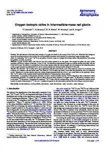
Fig. 1. Synthetic spectrum of 12 C14 N over the whole optical domain (r = 1 AU, r˙ = 0). The y-axis shows the decimal logarithm of the relative intensities (arbitrary units). The blue bands below 5000 Å belong to the B-X system, the red bands to the A-X system. The model is described in Section 6. vide evidence for the 12 C/13 C and 14 N/15 N isotopic ratios being primordial in the parent molecule that produces CN. However, infrared measurements obtained before and after impact showed an enhanced C2 H6 /H2 O ratio, but an unchanged HCN/H2 O ratio relative to the quiescent (pre-impact) source (DiSanti & Mumma 2008). It may therefore be that non-altered CN-bearing material had not been reached by the impact. However, the processes that could affect the isotopic ratios are not the same as those affecting the relative amounts of volatiles near the surface. It is also possible that the nucleus is not differentiated in HCN. The 2007 outburst of the Jupiter Family comet 17P/Holmes allowed us to reconcile the HCN and CN data (Bockelée-Morvan et al. 2008a). Observation of J = 3 − 2 rotational lines of H12 C14 N, H12 C15 N and H13 C14 N yielded 14 N/15 N= 139 ± 26 while the measurements of the CN violet band gave 14 N/15 N= 165 ± 40. Moreover it appeared that the HCN ratios that had been published for Hale-Bopp were seriously overestimated. A reanalysis of the data gave 138 37 K for H2 O (Dello Russo et al. 2007) instead of the more usual 30 K found in other comets for several molecules (see, e.g., Kawakita 2005) may also indicate a peculiar comet. Additional measurements of the nitrogen isotopic ratio in CN and other nitrogen-bearing species in additional comets, especially chemically peculiar ones, are needed to shed more light into these issues. Acknowledgements. This paper includes data taken at the McDonald Observatory of the University of Texas at Austin, at the W. M. Keck Observatory, which is operated as a scientific partnership by the California Institute of Technology, the University of California, and the National Aeronautics and Space Administration, and at the Nordic Optical Telescope (NOT), European Northern Observatory, La Palma, Spain. IRAF is distributed by the National Optical Astronomy Observatory, which is operated by the Association of Universities for Research in Astronomy (AURA) under cooperative agreement with the National Science Foundation.

References A’Hearn, M.F., et al. 2005, Science, 310, 258 Allison, A.C., & Dalgarno, A. 1971, A&A, 13, 331 Anders, E. & Grevesse, N., 1989, Geochim. Cosmochim. Acta, 53, 197 Arpigny, C., Schulz, R., Manfroid et al., 2000, Bull. Amer. Astron. Soc., 32, 1074 Arpigny, C., Jehin, E., Manfroid et al., 2003, Science 301, 1522 Bauschlicher, C.W., Jr., Langhoff, S.R., & Taylor, P.R. 1988, ApJ, 332, 531 Biver, N., Bockelée-Morvan, D., Colom, P., et al. 2002, Earth Moon and Planets, 90, 5 Biver, N., Bockelée-Morvan, Crovisier, J., et al. 2006, A&A, 449, 1255 Bockelée-Morvan, D., & Crovisier, J. 1987, A&A, 187, 425 Bockelée-Morvan, D., Crovisier, J., Colom, P., & Despois, D. 1994, A&A, 287, 647 Bockelée-Morvan, D, Biver, N., Jehin, E. et al. 2008a, A&A, 679, 249 Bockelée-Morvan, D, Dello Russo, N., Jehin, E. et al. 2008b, LPI Contributions, 1405, 8190

8

Table 2. Observed comets.

Comet 122P/de Vicoa C/1996 B2 (Hyakutake) C/1995 O1 (Hale-Bopp)b,c 55P/Tempel-Tuttle C/1999 H1 (Lee) C/1999 S4 (LINEAR) d C/1999 T1 (McNaught-Hartley) C/2001 A2 (LINEAR) C/2000 WM1 (LINEAR)b 153P/Ikeya-Zhang a C/2002 X5 (Kudo-Fujikawa) C/2002 V1 (NEAT) C/2002 Y1 (Juels-Holvorcem) 88P/Howell d C/2002 T7 (LINEAR) C/2001 Q4 (NEAT) c C/2003 K4 (LINEAR) c 9P/Tempel 1 e 73P-B/Schwassmann-Wachmann 3 73P-C/Schwassmann-Wachmann 3 C/2006 M4 (SWAN) 17P/Holmes g 8P/Tuttle h C/2007 N3 (Lulin)

f f

TP (yyyy-mm-dd) 1995-10-06 1996-05-01 1997-04-01 1998-02-28 1999-07-11 2000-07-26 2000-12-13 2001-05-25 2002-01-23 2002-03-19 2003-01-29 2003-02-18 2003-04-13 2004-04-13 2004-04-23 2004-05-16 2004-10-14 2005-07-05 2006-06-08 2006-06-07 2006-09-29 2007-05-04 2008-01-27 2009-01-10

e 0.96271 0.99990 0.99509 0.90555 0.99974 1.00010 0.99986 0.99969 1.00025 0.99010 0.99984 0.99990 0.99715 0.56124 1.00048 1.00069 1.00030 0.51749 0.69350 0.69338 1.00018 0.43242 0.8198 1.00004

a (AU) 17.7 2296 186.0 10.3 2773 – 8502 2530 – 51.2 1175 1010 250.6 3.1 – – – 3.1 3.1 3.1 – 3.6 5.7 –

q (AU) 0.66 0.23 0.91 0.98 0.71 0.77 1.17 0.78 0.56 0.51 0.19 0.10 0.71 1.37 0.61 0.96 1.02 1.51 0.94 0.94 0.78 2.05 1.03 1.21

Aph (AU) 34.7 4591 371.1 19.7 5545 – 17000 5060 – 101.9 2350 2021 500.5 4.9 – – – 4.7 5.2 5.2 – 5.18 10.4 –

i (◦ ) 85 125 89 162 149 149 80 36 73 28 94 82 104 4 161 100 134 11 11 11 112 19 55 178

P (yr) 74.3 110000 2537 33.2 146000 – 780000 127000 – 366.5 40300 32100 3967 5.5 – – – 5.5 5.4 5.4 – 6.9 13.6 –

TJ 0.37 -0.34 0.04 -0.64 -0.90 – 0.23 0.88 – 0.88 -0.03 0.06 -0.23 2.95 – – – 2.97 2.78 2.78 – 2.86 1.60 –

Type L H HF SPI EXT L EXT I HF SPI EXT L NEW L EXT L EXT L NEW L EXT IP EXT L EXT L EXT I JF SPIV NEW L NEW L NEW L JF SPIV JF SPIII JF SPIII NEW L JF SPIV HF SPI NEW L

a Jehin et al. 2004 – b Arpigny et al. 2000, 2003 – c Manfroid et al. 2005 – d Hutsemékers et al. 2005 – e Jehin et al. 2006 – f Jehin et al. 2008 – g Bockelée-Morvan et al. 2008a – h Bockelée-Morvan et al. 2008b The elements are obtained from the JPL Solar System Dynamics website. T P is the epoch of the perihelion, e the eccentricity, q the perihelion distance in AU, Aph the aphelion distance, i the inclination on the ecliptic, P the period, T J the Tisserand parameter relative to Jupiter, the last columns give the classification according to Levison (1996) and Horner et al. (2003). The subdivision I-IV based on T J is given for the SP comets only, all others being of the sub-type I.

I L

SP-I SP-III

SP-IV

14

15

N/ N

250 200 150 100 40

60

80 12

100

120

140

13

C/ C Fig. 8. 14 N/15 N versus 12 C/13 C. Different symbols refer to different comet families. Small shifts have been introduced to reduce overlapping.

Cochran, A.L., & Cochran, W. D., 2002, Icarus, 157, 297 Dahmen, G., Wilson, T.L., & Matteucci, F. 1995, A&A, 295, 194

Dekker, H., D’Odorico, S., Kaufer, A., Delabre, B., & Kotzlowski, H. 2000, Proc. SPIE, 4008, 534 Delbouille, L., Roland, G., & Neven, L. 1973, Atlas photométrique du spectre solaire de 3000 a` 10000 Å, Univ. Liège Dello Russo, N.., Vervack, R. J., Weaver, H. A. et al. 2007, Nature, 448, 172 Disanti, M.A., & Mumma, M. J., 2008, Space Science Reviews, 70 Floss, C., Stadermann, F.J., Bradley, J.P. et al., 2006, Geochim. Cosmochim. Acta, 70, 2371 Gausset, L., Herzberg, G., Lagerqvist, A., & Rosen, B. 1965, ApJ, 142, 45 Horner, J., Evans, N.W., Bailey, M.E., & Asher, D.J., 2003, MNRAS, 343, 1057 Hübner, M., Castillo, M., Davies, P.B., & Röpcke, J. 2005, Spectrochim. Acta A, 61, 57 Hutsemékers, D., Manfroid, J., Jehin, et al., 2005, A&A, 440, L21 Jehin, E., Manfroid, J., Cochran, A.L., et al., 2004, ApJ, 613, L161 Jehin, E., Manfroid, J., Hutsemékers, D., et al., 2006, ApJ, 641, L145 Jehin, E., Manfroid, J., Hutsemékers, D., et al., 2009, EM&P, submitted Jehin, E., Manfroid, J., Kawakita, H. et al., 2008, LPI Contributions, 1405, 8319 Jessberger, E.K., & Kissel, J., 1991, IAU Colloq. 116: Comets in the post-Halley era, 167, 1075 Jewitt, D.C., Matthews, H.E., Owen, T., and Meier, R., 1997, Science 278, 90 Kawakita, H., Watanabe, J., Furusho, R., et al., 2005, ApJ, 623, L49 Kleine, M., Wyckoff, S., Wehinger, P., & Peterson, B.A. 1995, ApJ, 439, 1021 Kobayashi, H., Kawakita, H., Mumma, M.J., Bonev, B.P., et al., 2007, ApJ, 668, L75 Kurucz, R.L. 2005, Mem. Soc. Astron. Italiana Suppl., 8, 189 Labs, D., & Neckel, H. 1970, Sol. Phys., 15, 79 Levison, H.F., 1996, ASPC, 107, 173 Lu, R., Huang, Y., & Halpern, J.B. 1992, ApJ, 395, 710 Lis, D.C., Keene, J., Young, K. et al. 1997a, Icarus, 130, 355 Manfroid, J., Jehin, E., Hutsemékers, D., et al., 2005, A&A, 432, L5 McKeegan, K.D., Aléon, J., Bradley, J., et al., 2006, Science, 314, 1724 Meech, K.J., Ageorges, N., A’Hearn, M.F., et al., 2005, Science, 310, 265 Milam, S.N., Savage, C., Brewster, M.A., et al., 2005, ApJ, 634, 1126 Owen, T. 1973, ApJ, 184, 33

9

Table 3. Observational circumstances.

Run 1 2 3 4 5 6 7 8 9 10 11 12 13 14 15 16 17 18 19 20 21 22 23 24 25 26 27 28 29 30 31 32 33 34 35 36 37 38 39 40 41 42 43 44 45 46

JD 2 400 000+ 49993:49994 50151 50175 50367:50374 50544 50545:50551 50830:50831 51444 51720:51721 51731:51742 51932:51935 52114 52340:52341 52355:52356 52386 52647:52649 52689:52690 52705 52719 52788:52789 52883:52889 53113:53117 53127:53129 53130:53132 53131:53132 53132 53142:53149 53150:53153 53166:53169 53328:53329 53520 53523:53529 53553:53563 53555 53857:53860 53858:53860 53882:53883 53898 53937 54039 54398:54402 54402 54403:54404 54422:54423 54481:54500 54876:54877

Comet 122P/de Vico C/1996 B2 (Hyakutake) C/1996 B2 (Hyakutake) C/1995 O1 (Hale-Bopp) C/1995 O1 (Hale-Bopp) C/1995 O1 (Hale-Bopp) 55P/Tempel-Tuttle C/1999 H1 (Lee) C/1999 S4 (LINEAR) C/1999 S4 (LINEAR) C/1999 T1 (McNaught-Hartley) C/2001 A2-A (LINEAR) C/2000 WM1 (LINEAR) C/2000 WM1 (LINEAR) 153P/Ikeya-Zhang C/2002 V1 (NEAT) C/2002 X5 (Kudo-Fujikawa) C/2002 X5 (Kudo-Fujikawa) C/2002 V1 (NEAT) C/2002 Y1 (Juels-Holvorcem) C/2001 Q4 (NEAT) 88P/Howell 88P/Howell C/2001 Q4 (NEAT) C/2002 T7 (LINEAR) C/2003 K4 (LINEAR) 88P/Howell C/2002 T7 (LINEAR) C/2002 T7 (LINEAR) C/2003 K4 (LINEAR) 9P/Tempel 1 9P/Tempel 1 9P/Tempel 1 9P/Tempel 1 73P-B/Schwassmann-Wachmann 3 73P-C/Schwassmann-Wachmann 3 73P-B/Schwassmann-Wachmann 3 73P-C/Schwassmann-Wachmann 3 73P-C/Schwassmann-Wachmann 3 C/2006 M4 (SWAN) 17P/Holmes 17P/Holmes 17P/Holmes 17P/Holmes 8P/Tuttle C/2007 N3 (Lulin)

r (AU) 0.66 1.35 0.87 2.68:2.77 0.91 0.92:0.94 1.18:1.19 1.54 0.96:0.97 0.78:0.86 1.34:1.36 1.36 1.08:1.1 1.32:1.34 0.92 1.17:1.22 0.69:0.72 1.06 1.01 1.14:1.15 3.66:3.73 1.37 1.38:1.39 0.97 0.68:0.69 2.59 1.42:1.44 0.92:0.97 1.17:1.21 1.19:1.2 1.55 1.53:1.54 1.51 1.51 1.05:1.07 1.05:1.07 0.95 0.94 1.12 0.99 2.44:2.46 2.46 2.46 2.54 1.03:1.04 1.33

r˙ (km/s) -2.89:-1.75 -32.94:-32.93 -38.69:-38.68 -20.78:-20.62 2.98:3 4.04:7.47 -15.5:-15.28 24.94 -19.6:-19.3 -14.9:-7.4 12.81:13.44 23.59 28.25:28.26 27.83:27.88 29.22 -37.11:-36.51 42.6:43.03 37 39.76 24.09:24.18 -18.91:-18.8 0.89:1.5 3:3.27 -5.43:-4.84 15.8:16.7 -20.35 5.04:5.9 25.4:25.9 26.84:26.87 14.55:14.81 -4 -3.7:-3.1 -0.3:0.8 -9.1:-0.1 -11.76:-11.06 -11.77:-11.33 -4.17:-3.79 1.79 13.22 19.48:19.5 5 6.65 5 6.94 -4.34:3.13 10.72:11

∆ (AU) 0.99:1 0.53 0.27 3.02:3.04 1.39 1.41:1.49 0.35 0.85 1.15:1.19 0.44:0.79 1.29:1.3 0.42 1.23 1.23 0.41 0.83:0.84 0.86 0.98 1.6 1.55 3.36:3.45 1.66:1.67 1.64 0.32 0.56:0.6 2.35 1.61:1.62 0.38:0.48 0.95:1.06 1.51:1.52 0.75 0.76:0.78 0.88:0.93 0.89 0.09:0.11 0.1:0.11 0.15 0.25 0.49 1.02 1.63 1.63 1.62 1.64 0.35:0.62 0.53

˙ ∆ (km/s) -14.3:-12.87 -57.03:-56.96 53.08:53.14 3.81:5.94 18.52:18.55 20.23:24.83 -2.37:4.96 -13.13 -62.3:-61.9 -63.2:-40 -6.73:-4.87 21.92 0.12:0.28 -0.25:-0.12 -6.44:-6.39 7.86:8.32 -5.09:-2.5 29.3:29.5 42 -7.23:-7.18 -25.43:-23.55 -4.5:-4.09 -3.3:-3.15 -4.12:2.23 -65.59:-64.8 -43 -2.7:-2.6 51.94:59.3 64.03:64.45 -28.26:-28.2 5.09:5.2 5.3:6.3 8.9:10.3 9.1:9.4 -11.3:-9.19 -12.1:-11.2 12.31:12.53 13.1 7.26 13.2:13.3 -3.8:-2.6 -2.4 -2.2:-1.9 5:5.2 21.64:24.79 -43:-39.7

Spectro

N

2DCoudé 2DCoudé 2DCoudé 2DCoudé 2DCoudé SOFIN 2DCoudé 2DCoudé 2DCoudé 2DCoudé 2DCoudé 2DCoudé UVES UVES 2DCoudé UVES UVES UVES UVES UVES UVES UVES UVES UVES UVES UVES UVES UVES UVES UVES HIRES UVES UVES HIRES 2DCoudé 2DCoudé UVES UVES UVES 2DCoudé 2DCoudé HIRES 2DCoudé 2DCoudé UVES 2DCoude

4 2 3 17 3 23 2 1 2 14 11 1 4 4 3 4 3 3 1 4 4 4 3 10 4 1 4 6 5 2 3 6 20 14 2 3 3 1 1 2 5 1 2 7 6 17

Exp (ks) 3.9 3.6 5.4 30.6 2.8 32.5 3.6 1.8 3.6 22.8 16.4 1.8 6.2 6.3 3.6 8.2 5.1 5.4 0.6 7.2 23.4 14.4 10.8 20.6 3.7 4.3 14.5 15.6 15.7 3 3.6 32.4 147.6 13.6 2.1 5.4 10.8 4.8 5 3.6 2.7 0 2.4 12.6 24 30.6

R 60000 60000 200000 60000 200000 70000 60000 60000 60000 60000 60000 60000 80000 80000 60000 80000 80000 80000 80000 80000 80000 80000 80000 80000 80000 60000 80000 80000 80000 80000 47000 80000 80000 47000 60000 60000 80000 80000 80000 60000 60000 47000 60000 60000 80000 60000

For convenience the data are grouped in observing runs. r is the heliocentric distance in astronomical units (AU), r˙ the heliocentric radial velocity, ∆ is the geocentric distance, ∆˙ the topocentric radial velocity, ’Spectro’ the spectrograph used, N is the number of individual spectra, ‘Exp’ the total exposure time in thousands of seconds, R = ∆λ/λ the resolving power. The nominal size of the entrance slit of the spectrograph is given in arcsec. Specific values relative to individual spectra can be found in Table 8. Owen, T., Mahaffy, P.R., Niemann, H.B., et al., 2001, ApJ, 553, L77 Ram, R.S., Davis, S.P., Wallace, L., Engleman, R., et al., 2006, Journal of Molecular Spectroscopy, 237, 225 Rauer, H., Helbert, J., Arpigny, C. et al., 2003, A&A, 397, 1109 Rodgers, S.D., & Charnley, S.B., 2008, MNRAS, 385, L48 Sauval, J., Asplund, M., Grevesse, N., van Hemert, M.C., & Groenenboom, G.C., 2009, to be published in A&A Solc, M, Vanysek, V. & Kissel, J., 1987, A&A, 187, 385 Stawikowski, A., & Greenstein, J.L., 1964, ApJ140, 1280 Swings, P., 1941, Lick Obs. Bull., 19, 131 Tull, R.G., MacQueen, P.J., Sneden, C., & Lambert, D.L. 1995, PASP, 107, 251 Univ. of Toledo Press, Toledo, p. 499 Wielen, R., & Wilson, T.L., 1997, A&A, 326, 139 Wyckoff, S., Lindholm, E., Wehinger, P.A., et al., 1989, ApJ, 339, 488 Wyckoff, S., & Wehinger, P., 1988, Reports of Planetary Astronomy, NASA, 145 Wyckoff, S.,Kleine, M., Peterson, B., et al., 2000, ApJ, 535, 991 Xie, X., & Mumma, M.J. 1992, ApJ, 386, 720 Ziurys, L.M., Savage, C., Brewster, et al., 1999, ApJ 527, L67 Zucconi, J.M., & Festou, M.C., 1985, A&A, 150, 180

Slit (′′ ×′′ ) 1.2 × 8.2 1.2 × 8.2 1.2 × 8.2 1.2 × 8.2 1.2 × 8.2 0.4 × 3.8 1.2 × 8.2 1.2 × 8.2 1.2 × 8.2 1.2 × 8.2 1.2 × 8.2 1.2 × 8.2 0.45 × 8 0.45 × 8 1.2 × 8.2 0.45 × 8 0.45 × 8 : 12 0.45 × 8 0.45 × 8 0.4 × 8 0.45 × 8 0.44 × 8 0.44 × 8 0.44 × 8 0.44 × 8 0.6 × 8 0.44 × 8 0.40 : 0.44 × 8 0.44 × 8 0.44 × 10 0.8 × 7 0.44 × 10 0.44 × 10 0.8 × 7 1.2 × 8.2 1.2 × 8.2 0.6 × 10 1 × 10 0.6 × 10 1.2 × 8.2 1.2 × 8.2 0.8 × 7 1.2 × 8.2 1.2 × 8.2 0.44 × 10 1.2 × 8.2

10

Table 4. Isotopic ratios in CN. Runs

Comet

12

C/13 C

14

1 2 3 4 5 6 7 8 9,10 11 12 13,14 15 17,18 16,19 20 21 22,23 24 25,28,29 26 30 31,34 32,33 35 36 37 38,39 40 41-44 41,43,44 42 45 46

122P/de Vico C/1996 B2 (Hyakutake) C/1996 B2 (Hyakutake) C/1995 O1 (Hale-Bopp) C/1995 O1 (Hale-Bopp) C/1995 O1 (Hale-Bopp) 55P/Tempel-Tuttle C/1999 H1 (Lee) C/1999 S4 (LINEAR) C/1999 T1 (McNaught-Hartley) C/2001 A2-A (LINEAR) C/2000 WM1 (LINEAR) 153P/Ikeya-Zhang C/2002 X5 (Kudo-Fujikawa) C/2002 V1 (NEAT) C/2002 Y1 (Juels-Holvorcem) C/2001 Q4 (NEAT) 88P/Howell C/2001 Q4 (NEAT) C/2002 T7 (LINEAR) C/2003 K4 (LINEAR) C/2003 K4 (LINEAR) 9P/Tempel 1 9P/Tempel 1 73P-B/Schwassmann-Wachmann 3 73P-C/Schwassmann-Wachmann 3 73P-B/Schwassmann-Wachmann 3 73P-C/Schwassmann-Wachmann 3 C/2006 M4 (SWAN) 17P/Holmes 17P/Holmes 17P/Holmes 8P/Tuttle C/2007 N3 (Lulin)

90 ± 10 ≥ 60 ≥ 50 80 ± 25 90 ± 20 100 ± 30 − ≥ 60 90 ± 30 80 ± 20 ≥ 60 100 ± 20 80 ± 30 90 ± 20 100 ± 20 90 ± 20 70 ± 30 90 ± 15 90 ± 15 85 ± 20 80 ± 20 90 ± 20 110 ± 20 95 ± 15 − − 100 ± 30 100 ± 20 95 ± 25 90 ± 20 ≥ 10 95 ± 20 90 ± 20 105 ± 40

N/15 N

145 ± 20 ≥ 60 ≥ 50 130 ± 40 150 ± 30 135 ± 40 − ≥ 60 150 ± 50 160 ± 50 ≥ 60 150 ± 30 140 ± 50 130 ± 20 160 ± 35 150 ± 35 130 ± 40 140 ± 20 135 ± 20 160 ± 25 150 ± 35 145 ± 25 170 ± 35 145 ± 20 − − 210 ± 50 220 ± 40 145 ± 50 165 ± 35 ≥ 10 165 ± 40 150 ± 30 150 ± 50

Reference Jehin et al. 2004 Manfroid et al. 2005 Manfroid et al. 2005 Manfroid et al. 2005 Hutsemékers et al. 2005 Arpigny et al. 2000, 2003 Jehin et al. 2004

Manfroid et al. 2005 Hutsemékers et al. 2005 Manfroid et al. 2005 Manfroid et al. 2005 Manfroid et al. 2005 Jehin et al. 2006 Jehin et al. 2006 Jehin et al. 2008 Jehin et al. 2008

Bockelée-Morvan et al. 2008a Bockelée-Morvan et al. 2008b

For convenience the data are grouped in observing runs as defined in Table 3. References are given when these are not first determinations, in italics if the values have been revised.

Table 7. Isotopic ratios in CN at various nucleocentric distances. The C/2002 T7 (LINEAR) data include spectra taken at up to 180 000 km but are strongly weighted for the range 24 000 − 45 000 km. Comet

Distance (km)

12

C/13 C

C/2001 Q4 (NEAT) C/2001 Q4 (NEAT) C/2001 Q4 (NEAT) C/2002 T7 (LINEAR) C/2002 T7 (LINEAR)

0 − 3 000 25 000 50 000 0 − 2 000 24 000 − 180 000

90 ± 20 95 ± 20 90 ± 20 85 ± 20 80 ± 25

14

N/15 N

135 ± 25 135 ± 25 145 ± 25 155 ± 25 165 ± 30

11

350

I L SP-I SP-III SP-IV

300

14

15

N/ N

250 200 150 100 50 0 200

100

12

13

C/ C

150

50 0 0.5

1 1.5 2 heliocentric distance (au)

3

4

Fig. 7. 12 C/13 C and 14 N/15 N versus the heliocentric distance. The horizontal lines show the mean values (91.0 and 147.8, respectively). Different symbols refer to different comet families.

3880 3878 3874 3876 wavelength (Å) 3872 3870 0.00

0.20

0.60

0.80

1.00

0.00

0.20

0.40

0.60

0.80

0.40 intensity

1.00

3858

3860

3862

C/2001 Q4 (NEAT)

3864

3866

3868

12

intensity

Fig. 9. Spectra of comet C/2001 Q4 (NEAT) obtained close to the nucleus (solid line) and at about 50000 km (green dashes). The positions of spatially peaked features appearing only in the nucleus spectrum are shown by dots. CH lines are indicated by + symbols. The upper (red) vertical ticks indicate the position of the main lines of 13 C14 N the lower (blue) ticks indicate the position of the main lines of 12 C15 N. The intensity scale is in relative units.

13

Table 5. Lines not identified as CN within the 3857–3880 Å range. Most are not yet identified.

λ (Å) 3857.36 3857.50 3857.58 3858.16 3858.90 3859.02 3859.46 3861.03 3861.68 3862.73 3863.71 3864.41 3865.40 3866.19 3866.28 3867.08 3867.92 3868.27 3873.14 3875.95 3877.09 3877.20 3877.47 3877.56 3877.65 3878.00 3878.40 3878.49 3878.57 3878.91 3879.36

Identification

CH R1 J ′′ = 3.5 CH R2 J ′′ = 1.5

CH R1 J ′′ = 2.5

Table 6. Average isotopic ratios. The weighted mean is computed for a variety of groups : all data, all data excluding 73P/Schwassmann-Wachmann 3 B and C, and each of the categories of Levison (JF, HF, EXT, NEW) or Horner et al. (SP, I, L). Group All comets All without S-W 3 JF JF without S-W Non JF (Oort) HF EXT NEW SPI SPIII SPIV I L

12

C/13 C 91.1 ± 3.7 90.6 ± 3.8 97.2 ± 7.6 96.3 ± 8.6 89.1 ± 4.2 90.0 ± 8.4 89.0 ± 6.9 89.1 ± 6.8 90.0 ± 8.4 100.0 ± 15.1 96.3 ± 8.6 88.2 ± 9.3 89.3 ± 5.8

14

N/15 N 147.8 ± 5.6 145.2 ± 5.6 156.8 ± 12.2 146.4 ± 12.4 144.0 ± 6.5 146.5 ± 15.1 141.3 ± 10.7 145.3 ± 9.5 146.5 ± 15.1 216.1 ± 27.3 146.4 ± 12.4 142.8 ± 14.8 143.8 ± 8.1

, Online Material p 1

Online Material

, Online Material p 2 x5

The analysis is done either by profile fitting around λ = 0 or by direct integration. In the latter case we write Z ∆λ/2 X Z ∆λ/2 X [ wi O(λ+λi )−C]δλ = α wi S 2 (λ+λi )δλ(A.2)

1.00

intensity

0.80 0.60

−∆λ/2

0.40 0.20

−∆λ/2

i

13

i

Fig. A.1. Coadded observed (solid line) and synthetic (with and without the rare isotopologues) spectra of comet C/2002 X5 (Kudo-Fujikawa). The upper panel is centered on 13 C14 N lines (in this instance, R1–R6, R14 and R16), the lower one on 12 C15 N lines (R1–R5, R11–R13, R15–R17). The large number of useable isotopic lines is allowed by the good quality of the spectra used in the combination. Intensity is in arbitrary units.

for the C N lines, and an equivalent formula for the 12 C15 N lines. The choice of the lines i depends on the quality of the spectra and on particular circumstances, especially the heliocentric distance. Figures 3 and 4 shows that the width of the envelope of the CN band decreases at large r. The relative intensity of the lines of high quantum number drops rapidly. Many lines could be used efficiently for the coadded profiles of comets de Vico or X5 (Fig. A.1), up to 11 for 12 C15 N and 8 for 13 C14 N. On the contrary, at large r, a few lines dominate overwhelmingly. As shown in Section 7, some blends may become less troublesome far from the nucleus. R lines of 13 C14 N and 12 C15 N with low quantum numbers are slightly blended and also – depending on the spectral resolution – with the corresponding R line of 12 C14 N. An additional difficulty is the presence of faint lines of the B-X (0-0) band of CH. This region of the spectrum needs special care (e.g., some iterative procedure) and may have to be ignored for the lowest quality spectra.

Appendix A: Estimating the isotopic ratios

Appendix B: Averages

0.00 −1

−0.5

0

0.5

1

−1

−0.5

0 wavelength (Å)

0.5

1

3.00

intensity

2.50 2.00 1.50 1.00 0.50 0.00

14

xi with errors ei Because of uncertainties in the models and systematic errors in While weighted averages of measurements P −2 P −2 (i = 1, . . . , n) are easily defined as m = x e i i the observations, the parameters α and β (Eq. 5) cannot be estii / i ei , estimating the resulting error on this value is less obvious. The global mated directly. Additional parameters are required to deal with the exact central wavelength of the lines, and the exact level of a data set is far from homogeneous. Systematic errors affect the various data sets in different ways. The instrumentation and the possible residual background Ck (λ). The spectra are divided into small domains surrounding the circumstances are never identical. Two estimates of the standard central wavelength λi of the most intense, unblended R lines of error S are sometimes used : 13 14 P C N and 12 C15 N, i.e., regions where αS k,2 (λ) or βS k,3 (λ) ≫ (xi − m)2 e−2 i S k,1 (λ). This is necessary because the accuracy of the 12 C14 N S 12 = i (B.1) P −2 (n − 1) e i i model is not perfect, especially in the wings of intense lines. Lines of other molecules must also be avoided, e.g., an unidenand tified feature at λ ∼ 3867.92 Å precludes the use of the R10 line X 12 15 of C N close to the nucleus (see Section 7). e−2 (B.2) S 22 = 1/ i . The line profile of the strongest lines can be fitted by a i Gaussian, or their intensity can be estimated by direct integraThey are not satisfying, particularly for a small data set. tion, providing sets of α and β which can then be averaged. Equation B.1 does not take properly into account the individual However, in order to reduce the number of free parameerrors, except for the weighting factors, so that a few xi with ters, we used a different procedure. Instead of fitting separately large e but grouped by chance around m would give an unrealisi O(λ) − Ci over the intervals [λi − ∆λ/2, λi + ∆λ/2], we superimpose the profiles by shifting the line centers to λ = 0, opti- tically small S 1 . On the other hand Eq. B.2 does not take into acmally coadd them, and fit the resulting profile over the resulting count the inter-group variations which can be large in the case of domain [−∆λ/2, ∆λ/2] (see Fig. A.1). Hence, dropping the sub- systematic effects. The larger of S 1 and S 2 may be taken, but we choose a different approach by simulating the xi as the average script k, we write, for the 13 C14 N lines, of ni individual observations yi, j ( j = 1, . . . , ni ) with a standard X X X ei . The weighting is obtained by taking ni proportional wi [O(λ+λi )−Ci ] ≡ wi O(λ+λi )−C = α wi S 2 (λ+λi )(A.1) deviation −2 to e i.e., the standard deviation is the same for each data set, i i i i σi = σ and ni = σ2 e−2 i . It is then possible to combine several and the corresponding formula with S 3 and β forP the 12 C15 N xi by merging their respective data sets. The mean value is the lines. The Ci s merge into a single free parameter i wi Ci ≡ C. same as above and the standard deviation of the mean is given The weight factor wi is estimated from the expected intensity by f (λi )Ii of line i in the SN-normalized spectrum (Eqs. P 2,3).  2P P P P 1/2 The width of the observed “coadded” profile Pi wi O(λ + λi )  σ i (ni − 1) + i ni x2i − ( i xi ni )2 / i ni   . e =  (B.3) P P is found P to be equal to that of the synthetic profile i wi S 2 (λ+λi ) i ni ( i ni − 1) (or i wi S 3 (λ+λi )) and it is symmetric about zero. This confirms that the identification of the 13 C14 N and 12 C15 N lines is correct, For large σ, this is equivalent to Eq. B.2, i.e., the result is as well as the theoretical wavelengths adopted for them. dominated by the internal dispersion of each data set. Choosing

, Online Material p 3 a reasonable value of σ is thus critical. We adopt the value of σ yielding the smallest realistic samples, min(ni ) = 2. This gives the largest, conservative estimates of the errors.

Appendix C: Spectra

3874 3872 3870 3868 wavelength (Å) 3866 3864 3862

0.00

0.01

0.03

0.04

0.00 3862 0.05

0.20

0.40

0.60

0.80

0.02 intensity

1.00

16

15

3864

14

13

3866

12

11

10

3868

9

122P/de Vico

8

7

3870

6

5

4

3872

3

2

12 14

C N obs syn

1

3874

0


intensity

Fig. C.1. Observed (2DCoudé) and synthetic (dotted) spectra of comet 122P/de Vico. In this and the following graphs, the upper (red) ticks indicate the position of the major R lines of 13 C14 N the lower (blue) ticks indicate the position of the major R lines of 12 15 C N. The corresponding quantum numbers are indicated in the upper panel midway between the strong 12 C14 N lines and the faint isotopic lines. The intensity scale is in relative units.

12 14

1.00

C N obs syn

intensity

0.80

0.60

16

15

14

13

12

11

10

9

8

7

6

5

4

3

2

1

0

0.40

0.20

0.00 3862 0.05

3864

3866

3864

3866

3868

3870

3872

3874

3870

3872

3874

0.04

intensity

0.03

0.02

0.01

0.00 3862

3868 wavelength (Å)


Fig. C.2. Observed (2DCoudé) and synthetic (dotted) spectra of comet C/1996 B2 (Hyakutake)

C/1996 B2 (Hyakutake)

12 14

1.00

C N obs syn

intensity

0.80

0.60

16

15

14

13

12

11

10

9

8

7

6

5

4

3

2

1

0

0.40

0.20

0.00 3862 0.05

3864

3866

3864

3866

3868

3870

3872

3874

3870

3872

3874

0.04

intensity

0.03

0.02

0.01

0.00 3862



Fig. C.3. Observed (2DCoudé) and synthetic (dotted) spectra of comet C/1996 B2 (Hyakutake)

C/1996 B2 (Hyakutake)

12 14

1.00

C N obs syn

intensity

0.80

0.60

16

15

14

13

12

11

10

9

8

7

6

5

4

3

2

1

0

0.40

0.20

0.00 3862 0.05

3864

3866

3864

3866

3868

3870

3872

3874

3870

3872

3874

0.04

intensity

0.03

0.02

0.01

0.00 3862



Fig. C.4. Observed (2DCoudé) and synthetic (dotted) spectra of comet C/1995 O1 (Hale-Bopp)

C/1995 O1 (Hale−Bopp)

12 14

1.00

C N obs syn

intensity

0.80

0.60

16

15

14

13

12

11

10

9

8

7

6

5

4

3

2

1

0

0.40

0.20

0.00 3862 0.05

3864

3866

3864

3866

3868

3870

3872

3874

3870

3872

3874

0.04

intensity

0.03

0.02

0.01

0.00 3862



Fig. C.5. Observed (2DCoudé) and synthetic (dotted) spectra of comet C/1995 O1 (Hale-Bopp)


12 14

1.00

C N obs syn

intensity

0.80

0.60

16

15

14

13

12

11

10

9

8

7

6

5

4

3

2

1

0

0.40

0.20

0.00 3862 0.05

3864

3866

3864

3866

3868

3870

3872

3874

3870

3872

3874

0.04

intensity

0.03

0.02

0.01

0.00 3862



Fig. C.6. Observed (SOFIN) and synthetic (dotted) spectra of comet C/1995 O1 (Hale-Bopp)


12 14

1.00

C N obs syn

intensity

0.80

0.60

16

15

14

13

12

11

10

9

8

7

6

5

4

3

2

1

0

0.40

0.20

0.00 3862 0.05

3864

3866

3864

3866

3868

3870

3872

3874

3870

3872

3874

0.04

intensity

0.03

0.02

0.01

0.00 3862



Fig. C.7. Observed (2DCoudé) and synthetic (dotted) spectra of comet 55P/Tempel-Tuttle

55P/Tempel−Tuttle

12 14

1.00

C N obs syn

intensity

0.80

0.60

16

15

14

13

12

11

10

9

8

7

6

5

4

3

2

1

0

0.40

0.20

0.00 3862 0.05

3864

3866

3864

3866

3868

3870

3872

3874

3870

3872

3874

0.04

intensity

0.03

0.02

0.01

0.00 3862



Fig. C.8. Observed (2DCoudé) and synthetic (dotted) spectra of comet C/1999 H1 (Lee)

C/1999 H1 (Lee)

12 14

1.00

C N obs syn

intensity

0.80

0.60

16

15

14

13

12

11

10

9

8

7

6

5

4

3

2

1

0

0.40

0.20

0.00 3862 0.05

3864

3866

3864

3866

3868

3870

3872

3874

3870

3872

3874

0.04

intensity

0.03

0.02

0.01

0.00 3862



Fig. C.9. Observed (2DCoudé) and synthetic (dotted) spectra of comet C/1999 S4 (LINEAR)

C/1999 S4 (LINEAR)

12 14

1.00

C N obs syn

intensity

0.80

0.60

16

15

14

13

12

11

10

9

8

7

6

5

4

3

2

1

0

0.40

0.20

0.00 3862 0.05

3864

3866

3864

3866

3868

3870

3872

3874

3870

3872

3874

0.04

intensity

0.03

0.02

0.01

0.00 3862



Fig. C.10. Observed (2DCoudé) and synthetic (dotted) spectra of comet C/1999 T1 (McNaught-Hartley)

C/1999 T1 (McNaught−Hartley)

12 14

1.00

C N obs syn

intensity

0.80

0.60

16

15

14

13

12

11

10

9

8

7

6

5

4

3

2

1

0

0.40

0.20

0.00 3862 0.05

3864

3866

3864

3866

3868

3870

3872

3874

3870

3872

3874

0.04

intensity

0.03

0.02

0.01

0.00 3862



Fig. C.11. Observed (2DCoudé) and synthetic (dotted) spectra of comet C/2001 A2-A (LINEAR)

C/2001 A2−A (LINEAR)

12 14

1.00

C N obs syn

intensity

0.80

0.60

16

15

14

13

12

11

10

9

8

7

6

5

4

3

2

1

0

0.40

0.20

0.00 3862 0.05

3864

3866

3864

3866

3868

3870

3872

3874

3870

3872

3874

0.04

intensity

0.03

0.02

0.01

0.00 3862



Fig. C.12. Observed (UVES) and synthetic (dotted) spectra of comet C/2000 WM1 (LINEAR)

C/2000 WM1 (LINEAR)

12 14

1.00

C N obs syn

intensity

0.80

0.60

16

15

14

13

12

11

10

9

8

7

6

5

4

3

2

1

0

0.40

0.20

0.00 3862 0.05

3864

3866

3864

3866

3868

3870

3872

3874

3870

3872

3874

0.04

intensity

0.03

0.02

0.01

0.00 3862



Fig. C.13. Observed (2DCoudé) and synthetic (dotted) spectra of comet 153P/Ikeya-Zhang

153P/Ikeya−Zhang

12 14

1.00

C N obs syn

intensity

0.80

0.60

16

15

14

13

12

11

10

9

8

7

6

5

4

3

2

1

0

0.40

0.20

0.00 3862 0.05

3864

3866

3864

3866

3868

3870

3872

3874

3870

3872

3874

0.04

intensity

0.03

0.02

0.01

0.00 3862



Fig. C.14. Observed (UVES) and synthetic (dotted) spectra of comet C/2002 X5 (Kudo-Fujikawa)

C/2002 X5 (Kudo−Fujikawa)

12 14

1.00

C N obs syn

intensity

0.80

0.60

16

15

14

13

12

11

10

9

8

7

6

5

4

3

2

1

0

0.40

0.20

0.00 3862 0.05

3864

3866

3864

3866

3868

3870

3872

3874

3870

3872

3874

0.04

intensity

0.03

0.02

0.01

0.00 3862



Fig. C.15. Observed (UVES) and synthetic (dotted) spectra of comet C/2002 V1 (NEAT)

C/2002 V1 (NEAT)

12 14

1.00

C N obs syn

intensity

0.80

0.60

16

15

14

13

12

11

10

9

8

7

6

5

4

3

2

1

0

0.40

0.20

0.00 3862 0.05

3864

3866

3864

3866

3868

3870

3872

3874

3870

3872

3874

0.04

intensity

0.03

0.02

0.01

0.00 3862



Fig. C.16. Observed (UVES) and synthetic (dotted) spectra of comet C/2002 Y1 (Juels-Holvorcem)

C/2002 Y1 (Juels−Holvorcem)

12 14

1.00

C N obs syn

intensity

0.80

0.60

16

15

14

13

12

11

10

9

8

7

6

5

4

3

2

1

0

0.40

0.20

0.00 3862 0.05

3864

3866

3864

3866

3868

3870

3872

3874

3870

3872

3874

0.04

intensity

0.03

0.02

0.01

0.00 3862



Fig. C.17. Observed (UVES) and synthetic (dotted) spectra of comet 88P/Howell

88P/Howell

12 14

1.00

C N obs syn

intensity

0.80

0.60

16

15

14

13

12

11

10

9

8

7

6

5

4

3

2

1

0

0.40

0.20

0.00 3862 0.05

3864

3866

3864

3866

3868

3870

3872

3874

3870

3872

3874

0.04

intensity

0.03

0.02

0.01

0.00 3862



Fig. C.18. Observed (UVES) and synthetic (dotted) spectra of comet C/2002 T7 (LINEAR)

C/2002 T7 (LINEAR)

12 14

1.00

C N obs syn

intensity

0.80

0.60

16

15

14

13

12

11

10

9

8

7

6

5

4

3

2

1

0

0.40

0.20

0.00 3862 0.05

3864

3866

3864

3866

3868

3870

3872

3874

3870

3872

3874

0.04

intensity

0.03

0.02

0.01

0.00 3862



Fig. C.19. Observed (UVES) and synthetic (dotted) spectra of comet C/2001 Q4 (NEAT)

C/2001 Q4 (NEAT)

12 14

1.00

C N obs syn

intensity

0.80

0.60

16

15

14

13

12

11

10

9

8

7

6

5

4

3

2

1

0

0.40

0.20

0.00 3862 0.05

3864

3866

3864

3866

3868

3870

3872

3874

3870

3872

3874

0.04

intensity

0.03

0.02

0.01

0.00 3862



Fig. C.20. Observed (UVES) and synthetic (dotted) spectra of comet C/2001 Q4 (NEAT)

C/2001 Q4 (NEAT)

12 14

1.00

C N obs syn

intensity

0.80

0.60

16

15

14

13

12

11

10

9

8

7

6

5

4

3

2

1

0

0.40

0.20

0.00 3862 0.05

3864

3866

3864

3866

3868

3870

3872

3874

3870

3872

3874

0.04

intensity

0.03

0.02

0.01

0.00 3862



Fig. C.21. Observed (UVES) and synthetic (dotted) spectra of comet C/2003 K4 (LINEAR)

C/2003 K4 (LINEAR)

12 14

1.00

C N obs syn

intensity

0.80

0.60

16

15

14

13

12

11

10

9

8

7

6

5

4

3

2

1

0

0.40

0.20

0.00 3862 0.05

3864

3866

3864

3866

3868

3870

3872

3874

3870

3872

3874

0.04

intensity

0.03

0.02

0.01

0.00 3862



Fig. C.22. Observed (UVES) and synthetic (dotted) spectra of comet C/2003 K4 (LINEAR)

C/2003 K4 (LINEAR)

12 14

1.00

C N obs syn

intensity

0.80

0.60

16

15

14

13

12

11

10

9

8

7

6

5

4

3

2

1

0

0.40

0.20

0.00 3862 0.05

3864

3866

3864

3866

3868

3870

3872

3874

3870

3872

3874

0.04

intensity

0.03

0.02

0.01

0.00 3862



Fig. C.23. Observed (HIRES) and synthetic (dotted) spectra of comet 9P/Tempel 1

9P/Tempel 1

12 14

1.00

C N obs syn

intensity

0.80

0.60

16

15

14

13

12

11

10

9

8

7

6

5

4

3

2

1

0

0.40

0.20

0.00 3862 0.05

3864

3866

3864

3866

3868

3870

3872

3874

3870

3872

3874

0.04

intensity

0.03

0.02

0.01

0.00 3862



Fig. C.24. Observed (UVES) and synthetic (dotted) spectra of comet 9P/Tempel 1

9P/Tempel 1

12 14

1.00

C N obs syn

intensity

0.80

0.60

16

15

14

13

12

11

10

9

8

7

6

5

4

3

2

1

0

0.40

0.20

0.00 3862 0.05

3864

3866

3864

3866

3868

3870

3872

3874

3870

3872

3874

0.04

intensity

0.03

0.02

0.01

0.00 3862



Fig. C.25. Observed (UVES) and synthetic (dotted) spectra of comet 73P-B/Schwassmann-Wachmann 3

73P−C/Schwassmann−Wachmann 3

12 14

1.00

C N obs syn

intensity

0.80

0.60

16

15

14

13

12

11

10

9

8

7

6

5

4

3

2

1

0

0.40

0.20

0.00 3862 0.05

3864

3866

3864

3866

3868

3870

3872

3874

3870

3872

3874

0.04

intensity

0.03

0.02

0.01

0.00 3862



Fig. C.26. Observed (2DCoudé) and synthetic (dotted) spectra of comet 73P-B/Schwassmann-Wachmann 3

73P−C/Schwassmann−Wachmann 3

12 14

1.00

C N obs syn

intensity

0.80

0.60

16

15

14

13

12

11

10

9

8

7

6

5

4

3

2

1

0

0.40

0.20

0.00 3862 0.05

3864

3866

3864

3866

3868

3870

3872

3874

3870

3872

3874

0.04

intensity

0.03

0.02

0.01

0.00 3862



Fig. C.27. Observed (UVES) and synthetic (dotted) spectra of comet 73P-C/Schwassmann-Wachmann 3

73P−B/Schwassmann−Wachmann 3

12 14

1.00

C N obs syn

intensity

0.80

0.60

16

15

14

13

12

11

10

9

8

7

6

5

4

3

2

1

0

0.40

0.20

0.00 3862 0.05

3864

3866

3864

3866

3868

3870

3872

3874

3870

3872

3874

0.04

intensity

0.03

0.02

0.01

0.00 3862



Fig. C.28. Observed (2DCoudé) and synthetic (dotted) spectra of comet 73P-C/Schwassmann-Wachmann 3

73P−B/Schwassmann−Wachmann 3

12 14

1.00

C N obs syn

intensity

0.80

0.60

16

15

14

13

12

11

10

9

8

7

6

5

4

3

2

1

0

0.40

0.20

0.00 3862 0.05

3864

3866

3864

3866

3868

3870

3872

3874

3870

3872

3874

0.04

intensity

0.03

0.02

0.01

0.00 3862



Fig. C.29. Observed (2DCoudé) and synthetic (dotted) spectra of comet C/2006 M4 (SWAN)

C/2006 M4 (SWAN)

12 14

1.00

C N obs syn

intensity

0.80

0.60

16

15

14

13

12

11

10

9

8

7

6

5

4

3

2

1

0

0.40

0.20

0.00 3862 0.05

3864

3866

3864

3866

3868

3870

3872

3874

3870

3872

3874

0.04

intensity

0.03

0.02

0.01

0.00 3862



Fig. C.30. Observed (HIRES) and synthetic (dotted) spectra of comet 17P/Holmes

17P/Holmes

12 14

1.00

C N obs syn

intensity

0.80

0.60

16

15

14

13

12

11

10

9

8

7

6

5

4

3

2

1

0

0.40

0.20

0.00 3862 0.05

3864

3866

3864

3866

3868

3870

3872

3874

3870

3872

3874

0.04

intensity

0.03

0.02

0.01

0.00 3862



Fig. C.31. Observed (2DCoudé) and synthetic (dotted) spectra of comet 17P/Holmes

17P/Holmes

12 14

1.00

C N obs syn

intensity

0.80

0.60

16

15

14

13

12

11

10

9

8

7

6

5

4

3

2

1

0

0.40

0.20

0.00 3862 0.05

3864

3866

3864

3866

3868

3870

3872

3874

3870

3872

3874

0.04

intensity

0.03

0.02

0.01

0.00 3862



Fig. C.32. Observed (2DCoudé) and synthetic (dotted) spectra of comet 8P/Tuttle

8P/Tuttle

12 14

1.00

C N obs syn

intensity

0.80

0.60

16

15

14

13

12

11

10

9

8

7

6

5

4

3

2

1

0

0.40

0.20

0.00 3862 0.05

3864

3866

3864

3866

3868

3870

3872

3874

3870

3872

3874

0.04

intensity

0.03

0.02

0.01

0.00 3862



Fig. C.33. Observed (2DCoudé) and synthetic (dotted) spectra of comet C/2007 N3 (Lulin)

C/2007 N3 (Lulin)

6000

600

5000

500

4000

400 intensity

intensity


3000

300

2000

200

1000

100

0 3863

3864

3865

3866

3867

3868

3869

3870

0 7953

3871

7954

7955

wavelength (Å)

7956

7957

7958

7959

7960

7961

wavelength (Å)

Fig. D.1. Small region of the B-X 0-0 band of the three CN isotopologues. The synthetic spectra were computed using isotopic abundances of 1, 1/89 and 1/145 for 12 C14 N (black), 13 C14 N (red) and 12 C15 N (blue), respectively, in the absence of collisional effects, and with r = 1 AU, r˙ = 0. The Gaussian profile has FWHM= 0.05 Å. The intensity scale is arbitrary, but coherent with the three following plots.

Fig. D.3. Same as Fig. D.1 for a region of the A-X 2-0 band. 1200

1000

800 intensity

600

600

500 400 400 intensity

200 300 0 9221

9222

9223

9224

9225

9226

9227

9228

9229

wavelength (Å)

200

Fig. D.4. Same as Fig. D.1 for a region of the A-X 1-0 band. 100

0 4202

4203

4204

4205

4206 4207 wavelength (Å)

4208

4209

4210

Fig. D.2. Same as Fig. D.1 for a region of the B-X 0-1 band.

Appendix D: Synthetic spectra

, Online Material p 38 Table 8. Individual spectra. r is the heliocentric distance in astronomical units (AU), ∆ the geocentric distance, Spectro the spectrograph used, MJD = JD − 2400000.5 the Modified Julian Day, Run the run number, Exp the exposure time in seconds, R the spectral resolution. Slit and Offset give the size of the entrance slit of the spectrograph and the offset from the nucleus. T and Q are the parameters used for the collisional effects in the synthetic spectra.

Comet deVico deVico deVico deVico Hyakutake Hyakutake Hyakutake Hyakutake Hyakutake HB HB HB HB HB HB HB HB HB HB HB HB HB HB HB HB HB HB HB HB HB HB HB HB HB HB HB HB HB HB HB HB HB HB HB HB HB HB HB HB HB HB HB TT TT Lee 1999S4 1999S4

r (AU) 0.66 0.66 0.66 0.66 1.36 1.36 0.87 0.87 0.87 2.77 2.77 2.77 2.77 2.76 2.76 2.76 2.76 2.76 2.70 2.70 2.70 2.70 2.68 2.68 2.68 2.68 0.92 0.92 0.92 0.92 0.92 0.92 0.92 0.92 0.93 0.93 0.93 0.93 0.93 0.93 0.93 0.93 0.93 0.93 0.94 0.94 0.94 0.94 0.94 0.94 0.94 0.94 1.19 1.18 1.54 0.97 0.96

∆ (AU) 1.00 1.00 0.99 0.99 0.54 0.54 0.28 0.28 0.28 3.02 3.02 3.02 3.02 3.03 3.03 3.03 3.03 3.03 3.04 3.04 3.04 3.04 3.04 3.04 3.04 3.04 1.40 1.40 1.40 1.42 1.42 1.43 1.43 1.43 1.44 1.44 1.44 1.45 1.45 1.45 1.45 1.47 1.47 1.47 1.48 1.48 1.48 1.48 1.49 1.49 1.49 1.49 0.36 0.36 0.85 1.19 1.16

mr 5.60 5.60 5.62 5.62 6.55 6.55 4.79 4.78 4.78 3.19 3.19 3.19 3.19 3.19 3.19 3.19 3.19 3.19 3.08 3.08 3.08 3.08 3.08 3.08 3.08 3.08 -1.12 -1.12 -1.12 -1.15 -1.15 -1.17 -1.17 -1.17 -1.19 -1.19 -1.19 -1.20 -1.20 -1.20 -1.10 -1.12 -1.12 -1.12 -1.14 -1.14 -1.14 -1.14 -1.16 -1.16 -1.16 -1.16 10.24 10.23 8.74 7.81 7.87

Spectro 2DCoudé 2DCoudé 2DCoudé 2DCoudé 2DCoudé 2DCoudé 2DCoudé 2DCoudé 2DCoudé 2DCoudé 2DCoudé 2DCoudé 2DCoudé 2DCoudé 2DCoudé 2DCoudé 2DCoudé 2DCoudé 2DCoudé 2DCoudé 2DCoudé 2DCoudé 2DCoudé 2DCoudé 2DCoudé 2DCoudé 2DCoudé 2DCoudé 2DCoudé SOFIN SOFIN SOFIN SOFIN SOFIN SOFIN SOFIN SOFIN SOFIN SOFIN SOFIN SOFIN SOFIN SOFIN SOFIN SOFIN SOFIN SOFIN SOFIN SOFIN SOFIN SOFIN SOFIN 2DCoudé 2DCoudé 2DCoudé 2DCoudé 2DCoudé

MJD 49993.488 49993.502 49994.475 49994.495 50151.467 50151.490 50175.090 50175.113 50175.134 50367.086 50367.111 50367.141 50367.165 50368.066 50368.091 50368.115 50368.138 50368.162 50373.062 50373.086 50373.110 50373.134 50374.057 50374.080 50374.103 50374.126 50544.068 50544.079 50544.112 50545.863 50545.886 50546.832 50546.839 50546.865 50547.836 50547.862 50547.887 50548.837 50548.856 50548.874 50548.893 50549.837 50549.855 50549.875 50550.836 50550.857 50550.877 50550.896 50551.834 50551.856 50551.874 50551.892 50830.104 50831.158 51444.219 51720.377 51721.362

Run 1 1 1 1 2 2 3 3 3 4 4 4 4 4 4 4 4 4 4 4 4 4 4 4 4 4 5 5 5 6 6 6 6 6 6 6 6 6 6 6 6 6 6 6 6 6 6 6 6 6 6 6 7 7 8 9 9

Exp (s) 600 600 1500 1200 1800 1800 1800 1800 1800 1800 1800 1800 1800 1800 1800 1800 1800 1800 1800 1800 1800 1800 1800 1800 1800 1800 120 900 1800 1814 2106 600 460 3838 1800 1800 1800 1200 1200 1200 1200 1200 1200 1200 1200 1516 1200 1199 1200 1200 1199 1200 1800 1800 1800 1800 1800

R 60000 60000 60000 60000 60000 60000 200000 200000 200000 60000 60000 60000 60000 60000 60000 60000 60000 60000 60000 60000 60000 60000 60000 60000 60000 60000 200000 200000 200000 70000 70000 70000 70000 70000 70000 70000 70000 70000 70000 70000 70000 70000 70000 70000 70000 70000 70000 70000 70000 70000 70000 70000 60000 60000 60000 60000 60000

Slit (′′ ×′′ ) 1.20 × 8.20 1.20 × 8.20 1.20 × 8.20 1.20 × 8.20 1.20 × 8.20 1.20 × 8.20 1.20 × 8.20 1.20 × 8.20 1.20 × 8.20 1.20 × 8.20 1.20 × 8.20 1.20 × 8.20 1.20 × 8.20 1.20 × 8.20 1.20 × 8.20 1.20 × 8.20 1.20 × 8.20 1.20 × 8.20 1.20 × 8.20 1.20 × 8.20 1.20 × 8.20 1.20 × 8.20 1.20 × 8.20 1.20 × 8.20 1.20 × 8.20 1.20 × 8.20 1.20 × 8.20 1.20 × 8.20 1.20 × 8.20 0.45 × 3.80 0.45 × 3.80 0.45 × 3.80 0.45 × 3.80 0.45 × 3.80 0.45 × 3.80 0.45 × 3.80 0.45 × 3.80 0.45 × 3.80 0.45 × 3.80 0.45 × 3.80 0.45 × 3.80 0.45 × 3.80 0.45 × 3.80 0.45 × 3.80 0.45 × 3.80 0.45 × 3.80 0.45 × 3.80 0.45 × 3.80 0.45 × 3.80 0.45 × 3.80 0.45 × 3.80 0.45 × 3.80 1.20 × 8.20 1.20 × 8.20 1.20 × 8.20 1.20 × 8.20 1.20 × 8.20

Offset (′′ ) 0 0 0 100 0 0 0 0 0 0 0 0 0 0 0 0 0 0 0 0 0 0 0 0 0 0 0 0 0 0 0 0 0 0 0 0 0 0 0 0 0 0 0 0 0 0 0 0 0 0 0 0 0 0 0 0 0

T (K) 410 410 410 400 230 230 390 340 380 140 130 – 240 – – 190 110 220 – – 170 200 200 – – 140 300 310 – 280 320 300 300 310 300 300 290 320 320 300 320 250 250 250 300 300 400 380 390 380 350 340 230 190 270 340 300

5 + log Q (s−1 ) 1.9 1.8 1.8 1.7 2.8 2.7 3.1 1.1 3.1 1.0 0.7 – 0.8 – – 0.7 0.1 0.9 – – 1.0 0.1 0.8 – – 0.9 3.2 1.9 – 3.0 3.2 3.0 3.2 2.9 2.9 3.2 3.0 3.1 3.2 3.1 3.0 2.7 2.8 3.0 3.0 2.6 3.2 3.0 2.2 3.2 2.7 3.0 1.7 1.9 1.2 1.9 1.9

, Online Material p 39 Table 8. continued.

Comet 1999S4 1999S4 1999S4 1999S4 1999S4 1999S4 1999S4 1999S4 1999S4 1999S4 1999S4 1999S4 1999S4 1999S4 1999T1 1999T1 1999T1 1999T1 1999T1 1999T1 1999T1 1999T1 1999T1 1999T1 1999T1 2001A2-A 2000WM1 2000WM1 2000WM1 2000WM1 2000WM1 2000WM1 2000WM1 2000WM1 IZ IZ IZ 2002X5 2002X5 2002X5 2002X5 2002X5 2002X5 2002V1 2002V1 2002V1 2002V1 2002V1 2002Y1 2002Y1 2002Y1 2002Y1 Howell Howell Howell Howell Howell Howell Howell Howell

r (AU) 0.86 0.85 0.80 0.80 0.80 0.80 0.79 0.79 0.79 0.78 0.78 0.78 0.78 0.78 1.34 1.34 1.34 1.34 1.34 1.34 1.36 1.36 1.36 1.36 1.36 1.36 1.08 1.08 1.10 1.10 1.33 1.33 1.34 1.34 0.92 0.92 0.92 0.70 0.72 0.72 1.06 1.06 1.06 1.22 1.22 1.18 1.18 1.01 1.14 1.14 1.16 1.16 1.37 1.37 1.37 1.37 1.38 1.39 1.39 1.42

∆ (AU) 0.80 0.76 0.52 0.52 0.52 0.52 0.49 0.46 0.46 0.44 0.44 0.44 0.44 0.44 1.31 1.31 1.30 1.30 1.30 1.30 1.30 1.30 1.30 1.30 1.30 0.43 1.24 1.24 1.24 1.24 1.24 1.24 1.24 1.24 0.42 0.42 0.42 0.87 0.86 0.86 0.99 0.99 0.99 0.83 0.83 0.84 0.84 1.60 1.56 1.56 1.55 1.55 1.68 1.67 1.67 1.67 1.65 1.65 1.64 1.63

mr 8.39 8.50 8.91 8.91 8.91 8.91 8.84 8.86 8.86 8.87 8.87 8.87 8.87 8.88 7.11 7.11 7.12 7.12 7.12 7.12 7.13 7.13 7.13 7.13 7.13 8.45 6.83 6.83 6.83 6.83 8.43 8.43 8.43 8.43 6.39 6.39 6.39 4.81 4.81 4.81 9.32 9.32 9.32 7.89 7.89 7.87 7.87 5.47 7.13 7.13 7.14 7.14 11.07 11.08 8.78 8.79 8.81 8.81 8.82 8.84

Spectro 2DCoudé 2DCoudé 2DCoudé 2DCoudé 2DCoudé 2DCoudé 2DCoudé 2DCoudé 2DCoudé 2DCoudé 2DCoudé 2DCoudé 2DCoudé 2DCoudé 2DCoudé 2DCoudé 2DCoudé 2DCoudé 2DCoudé 2DCoudé 2DCoudé 2DCoudé 2DCoudé 2DCoudé 2DCoudé 2DCoudé UVES UVES UVES UVES UVES UVES UVES UVES 2DCoudé 2DCoudé 2DCoudé UVES UVES UVES UVES UVES UVES UVES UVES UVES UVES UVES UVES UVES UVES UVES UVES UVES UVES UVES UVES UVES UVES UVES

MJD 51731.387 51732.390 51739.388 51739.414 51739.439 51739.459 51740.423 51741.443 51741.463 51742.359 51742.384 51742.419 51742.443 51742.463 51932.520 51932.537 51933.449 51933.476 51933.505 51933.549 51935.439 51935.468 51935.494 51935.522 51935.545 52114.341 52340.362 52340.381 52341.368 52341.387 52355.362 52355.380 52356.363 52356.382 52386.431 52386.447 52386.464 52689.013 52690.007 52690.020 52705.017 52705.039 52705.060 52647.037 52647.062 52649.031 52649.056 52719.985 52788.394 52788.416 52789.393 52789.415 53113.372 53114.364 53115.368 53117.371 53127.372 53128.363 53129.372 53142.358

Run 10 10 10 10 10 10 10 10 10 10 10 10 10 10 11 11 11 11 11 11 11 11 11 11 11 12 13 13 13 13 14 14 14 14 15 15 15 17 17 17 18 18 18 16 16 16 16 19 20 20 20 20 22 22 22 22 23 23 23 29

Exp (s) 1800 1800 1800 1800 1800 1200 1200 1800 1200 1800 1800 1800 1800 1200 1200 1200 1800 1800 1800 700 1800 1800 1800 1800 700 1800 1550 1550 1550 1550 1550 1550 1610 1610 1200 1200 1200 2000 1100 2000 1800 1800 1800 2100 2100 2100 1983 600 1800 1800 1800 1800 3600 3600 3600 3600 3600 3600 3600 3600

R 60000 60000 60000 60000 60000 60000 60000 60000 60000 60000 60000 60000 60000 60000 60000 60000 60000 60000 60000 60000 60000 60000 60000 60000 60000 60000 80000 80000 80000 80000 80000 80000 80000 80000 60000 60000 60000 80000 80000 80000 80000 80000 80000 80000 80000 80000 80000 80000 80000 80000 80000 80000 80000 80000 80000 80000 80000 80000 80000 80000

Slit (′′ ×′′ ) 1.20 × 8.20 1.20 × 8.20 1.20 × 8.20 1.20 × 8.20 1.20 × 8.20 1.20 × 8.20 1.20 × 8.20 1.20 × 8.20 1.20 × 8.20 1.20 × 8.20 1.20 × 8.20 1.20 × 8.20 1.20 × 8.20 1.20 × 8.20 1.20 × 8.20 1.20 × 8.20 1.20 × 8.20 1.20 × 8.20 1.20 × 8.20 1.20 × 8.20 1.20 × 8.20 1.20 × 8.20 1.20 × 8.20 1.20 × 8.20 1.20 × 8.20 1.20 × 8.20 0.45 × 8.00 0.45 × 8.00 0.45 × 8.00 0.45 × 8.00 0.45 × 8.00 0.45 × 8.00 0.45 × 8.00 0.45 × 8.00 1.20 × 8.20 1.20 × 8.20 1.20 × 8.20 0.45 × 8.00 0.45 × 12.00 0.45 × 12.00 0.45 × 8.00 0.45 × 8.00 0.45 × 8.00 0.45 × 8.00 0.45 × 8.00 0.45 × 8.00 0.45 × 8.00 0.45 × 8.00 0.40 × 8.00 0.40 × 8.00 0.40 × 8.00 0.40 × 8.00 0.44 × 8.00 0.44 × 8.00 0.44 × 8.00 0.44 × 8.00 0.44 × 8.00 0.44 × 8.00 0.44 × 8.00 0.44 × 8.00

Offset (′′ ) 0 0 0 0 0 0 0 0 0 0 0 0 0 0 0 0 0 0 0 0 0 0 0 0 0 0 10 10 10 6 2 2 1 1 0 0 52 0 20 20 0 3 3 0 0 0 0 0 0 0 3 3 0 0 0 0 0 0 0 0

T (K) 260 280 400 – 350 400 330 340 350 330 330 400 330 330 – – 300 310 – 270 – 320 270 250 260 270 270 270 270 290 290 300 290 310 310 310 320 400 330 330 300 270 270 310 310 320 300 330 310 340 380 380 260 250 220 260 260 250 240 270

5 + log Q (s−1 ) 2.0 1.9 1.7 – 1.1 1.7 0.1 1.2 1.0 1.1 0.9 0.8 0.1 1.2 – – 2.0 1.1 – 1.9 – 0.9 1.9 -0.4 1.9 1.8 0.1 0.1 0.1 0.1 1.0 1.0 1.1 1.0 2.1 1.2 1.9 1.9 1.2 1.2 1.5 1.2 1.2 1.2 1.2 1.2 1.2 1.9 1.2 1.6 1.2 1.1 1.0 1.2 1.0 1.1 1.2 1.2 1.2 1.2


Comet Howell Howell Howell 2002T7 2002T7 2002T7 2002T7 2002T7 2002T7 2002T7 2002T7 2002T7 2002T7 2002T7 2002T7 2002T7 2002T7 2002T7 2001Q4 2001Q4 2001Q4 2001Q4 2001Q4 2001Q4 2001Q4 2001Q4 2001Q4 2001Q4 2001Q4 2001Q4 2001Q4 2001Q4 2003K4 2003K4 2003K4 Tempel1 Tempel1 Tempel1 Tempel1 Tempel1 Tempel1 Tempel1 Tempel1 Tempel1 Tempel1 Tempel1 Tempel1 Tempel1 Tempel1 Tempel1 Tempel1 Tempel1 Tempel1 Tempel1 Tempel1 Tempel1 Tempel1 Tempel1 Tempel1 Tempel1

r (AU) 1.43 1.44 1.44 0.68 0.68 0.69 0.69 0.93 0.94 0.94 0.96 0.97 0.97 1.17 1.18 1.18 1.20 1.22 3.73 3.73 3.67 3.66 0.98 0.98 0.98 0.98 0.98 0.98 0.98 0.98 0.98 0.97 2.59 1.19 1.20 1.55 1.55 1.55 1.54 1.54 1.53 1.53 1.53 1.53 1.51 1.51 1.51 1.51 1.51 1.51 1.51 1.51 1.51 1.51 1.51 1.51 1.51 1.51 1.51 1.51

∆ (AU) 1.62 1.62 1.62 0.61 0.61 0.57 0.57 0.38 0.41 0.42 0.45 0.48 0.48 0.95 0.99 0.99 1.03 1.07 3.45 3.45 3.37 3.37 0.32 0.32 0.32 0.32 0.32 0.32 0.32 0.32 0.32 0.32 2.35 1.53 1.51 0.75 0.75 0.75 0.76 0.76 0.78 0.78 0.78 0.78 0.89 0.89 0.89 0.89 0.89 0.89 0.89 0.89 0.89 0.89 0.89 0.89 0.89 0.89 0.89 0.89

mr

Spectro

MJD

8.95 8.95 8.95 4.87 4.87 5.02 5.02 5.18 5.01 5.00 4.84 4.79 4.78 6.10 6.12 6.11 6.24 6.36 9.51 9.51 9.56 9.56 6.06 6.06 6.06 6.06 6.06 6.06 6.06 6.06 6.06 6.06 9.14 5.78 5.80 10.71 10.71 10.71 10.69 10.69 10.65 10.65 10.63 10.63 10.36 10.36 10.34 10.34 10.34 10.34 10.34 10.34 10.34 10.34 10.34 10.34 10.34 10.34 10.34 10.34

UVES UVES UVES UVES UVES UVES UVES UVES UVES UVES UVES UVES UVES UVES UVES UVES UVES UVES UVES UVES UVES UVES UVES UVES UVES UVES UVES UVES UVES UVES UVES UVES UVES UVES UVES HIRES HIRES HIRES UVES UVES UVES UVES UVES UVES UVES UVES UVES UVES HIRES HIRES HIRES HIRES HIRES HIRES HIRES HIRES HIRES HIRES HIRES HIRES

53146.371 53147.391 53149.361 53131.406 53131.421 53132.412 53132.424 53150.983 53151.976 53152.036 53152.970 53153.973 53153.986 53166.967 53167.967 53168.012 53168.983 53169.983 52883.293 52883.349 52889.236 52889.320 53130.958 53130.960 53130.962 53130.965 53130.967 53130.975 53131.066 53131.952 53131.991 53132.065 53132.343 53328.347 53329.344 53520.363 53520.378 53520.392 53523.016 53523.083 53528.025 53528.091 53529.033 53529.102 53553.955 53554.041 53554.954 53555.041 53555.238 53555.250 53555.258 53555.267 53555.278 53555.289 53555.300 53555.311 53555.322 53555.333 53555.344 53555.355

Run 29 29 29 25 25 28 28 30 30 30 30 30 30 31 31 31 31 31 21 21 21 21 24 24 24 24 24 24 24 26 26 26 27 32 32 33 33 33 34 34 34 34 34 34 35 35 35 35 36 36 36 36 36 36 36 36 36 36 36 36

Exp (s) 3600 2499 4900 1080 1080 800 800 3208 2677 1800 3900 487 3600 3600 3000 3000 3120 3000 4500 4500 7200 7200 120 120 120 120 600 7200 2185 1782 6300 2144 4380 1500 1500 1200 1200 1200 5400 5400 5400 5400 5400 5400 7200 7200 7200 7200 720 600 600 900 900 900 900 900 900 900 900 900

R 80000 80000 80000 80000 80000 80000 80000 80000 80000 80000 80000 80000 80000 80000 80000 80000 80000 80000 80000 80000 80000 80000 80000 80000 80000 80000 80000 80000 80000 80000 80000 80000 60000 80000 80000 47000 47000 47000 80000 80000 80000 80000 80000 80000 80000 80000 80000 80000 47000 47000 47000 47000 47000 47000 47000 47000 47000 47000 47000 47000

Slit (′′ ×′′ ) 0.44 × 8.00 0.44 × 8.00 0.44 × 8.00 0.44 × 8.00 0.44 × 8.00 0.44 × 8.00 0.44 × 8.00 0.44 × 8.00 0.40 × 8.00 0.40 × 8.00 0.44 × 8.00 0.40 × 8.00 0.44 × 8.00 0.44 × 8.00 0.44 × 8.00 0.44 × 8.00 0.44 × 8.00 0.44 × 8.00 0.45 × 8.00 0.45 × 8.00 0.45 × 8.00 0.45 × 8.00 0.44 × 8.00 0.44 × 8.00 0.44 × 8.00 0.44 × 8.00 0.44 × 8.00 0.44 × 8.00 0.44 × 8.00 0.44 × 8.00 0.44 × 8.00 0.44 × 8.00 0.60 × 8.00 0.44 × 10.00 0.44 × 10.00 0.86 × 7.00 0.86 × 7.00 0.86 × 7.00 0.44 × 10.00 0.44 × 10.00 0.44 × 10.00 0.44 × 10.00 0.44 × 10.00 0.44 × 10.00 0.44 × 10.00 0.44 × 10.00 0.44 × 10.00 0.44 × 10.00 0.86 × 7.00 0.86 × 7.00 0.86 × 7.00 0.86 × 7.00 0.86 × 7.00 0.86 × 7.00 0.86 × 7.00 0.86 × 7.00 0.86 × 7.00 0.86 × 7.00 0.86 × 7.00 0.86 × 7.00

Offset (′′ ) 0 0 0 5 5 110 110 0 0 0 70 70 70 70 245 245 245 245 0 0 0 0 2 3 13 108 108 217 13 110 216 13 0 0 0 0 0 0 0 0 0 0 0 0 1 1 1 1 0 0 0 0 0 0 0 0 0 0 0 0

T (K) 250 260 260 330 420 – – 350 310 340 330 370 340 290 310 290 290 310 160 130 140 – 350 330 420 – 330 330 420 330 400 330 200 320 330 350 380 380 320 290 310 290 320 310 300 280 – 210 420 310 210 200 260 240 210 210 230 230 – 230

5 + log Q (s−1 ) 1.2 1.2 1.2 1.2 1.8 – – 2.1 2.6 2.1 1.1 0.6 0.9 1.1 0.9 0.1 0.1 -0.3 0.1 0.7 0.8 – 2.0 1.2 0.9 – -0.0 0.1 1.0 0.1 0.8 1.2 0.1 1.7 1.7 1.2 1.0 1.1 1.2 1.2 1.2 1.2 1.2 1.2 0.8 0.1 – -0.4 3.2 3.2 1.8 1.7 2.2 1.8 1.2 1.2 1.2 1.2 – 1.2


Comet Tempel1 Tempel1 Tempel1 Tempel1 Tempel1 Tempel1 Tempel1 Tempel1 Tempel1 Tempel1 Tempel1 Tempel1 Tempel1 Tempel1 Tempel1 Tempel1 Tempel1 Tempel1 SW3-B SW3-B SW3-B SW3-B SW3-B SW3-C SW3-C SW3-C SW3-C SW3-C SWAN SWAN Holmes Holmes Holmes Holmes Holmes Holmes Holmes Holmes Holmes Holmes Holmes Holmes Holmes Holmes Holmes Tuttle Tuttle Tuttle Tuttle Tuttle Tuttle Lulin Lulin Lulin Lulin Lulin Lulin Lulin Lulin Lulin

r (AU) 1.51 1.51 1.51 1.51 1.51 1.51 1.51 1.51 1.51 1.51 1.51 1.51 1.51 1.51 1.51 1.51 1.51 1.51 1.05 1.07 0.95 0.95 0.95 1.06 1.07 1.07 0.94 1.13 1.00 1.00 2.44 2.44 2.45 2.45 2.46 2.46 2.46 2.46 2.54 2.54 2.54 2.54 2.54 2.54 2.54 1.04 1.04 1.03 1.03 1.03 1.03 1.33 1.33 1.33 1.33 1.33 1.33 1.33 1.33 1.33

∆ (AU) 0.89 0.89 0.90 0.90 0.90 0.90 0.91 0.91 0.91 0.92 0.92 0.92 0.93 0.93 0.93 0.93 0.94 0.94 0.10 0.12 0.15 0.16 0.16 0.10 0.11 0.12 0.25 0.50 1.02 1.02 1.63 1.63 1.63 1.63 1.63 1.63 1.62 1.62 1.64 1.64 1.64 1.64 1.64 1.64 1.64 0.36 0.36 0.52 0.52 0.62 0.62 0.53 0.53 0.53 0.53 0.53 0.53 0.53 0.53 0.53

mr 10.34 10.34 10.33 10.33 10.41 10.41 10.40 10.40 10.39 10.39 10.38 10.48 10.46 10.46 10.45 10.55 10.54 10.54 11.02 10.65 11.60 11.50 11.50 11.07 10.95 10.79 11.39 14.52 5.25 5.25 1.43 1.43 1.43 1.43 1.43 1.43 1.45 1.45 1.92 1.92 1.92 1.92 1.92 1.92 1.92 8.43 8.42 8.01 8.00 7.73 7.73 6.97 6.97 6.97 6.97 6.97 6.97 6.97 6.97 6.97

Spectro HIRES HIRES UVES UVES UVES UVES UVES UVES UVES UVES UVES UVES UVES UVES UVES UVES UVES UVES 2DCoudé 2DCoudé UVES UVES UVES 2DCoudé 2DCoudé 2DCoudé UVES UVES 2DCoudé 2DCoudé 2DCoudé 2DCoudé 2DCoudé 2DCoudé 2DCoudé HIRES 2DCoudé 2DCoudé 2DCoudé 2DCoudé 2DCoudé 2DCoudé 2DCoudé 2DCoudé 2DCoudé UVES UVES UVES UVES UVES UVES 2DCoudé 2DCoudé 2DCoudé 2DCoudé 2DCoudé 2DCoudé 2DCoudé 2DCoudé 2DCoudé

MJD 53555.372 53555.393 53555.955 53556.043 53557.007 53557.121 53557.955 53558.044 53558.952 53559.041 53559.954 53560.044 53560.952 53561.045 53561.953 53562.041 53562.955 53563.041 53857.209 53860.322 53882.367 53883.353 53883.398 53858.190 53859.212 53860.183 53898.369 53937.345 54039.052 54039.074 54398.400 54398.406 54401.290 54401.300 54402.362 54402.573 54403.362 54404.383 54422.366 54422.388 54422.410 54422.432 54423.253 54423.275 54423.297 54481.021 54481.071 54493.018 54493.071 54500.017 54500.070 54876.328 54876.351 54876.373 54876.395 54876.418 54876.440 54876.463 54876.486 54876.508

Run 36 36 37 37 37 37 37 37 37 37 37 37 37 37 37 37 37 37 38 40 41 41 41 39 39 39 42 43 44 44 45 45 45 45 45 46 47 47 48 48 48 48 48 48 48 49 49 49 49 49 49 50 50 50 50 50 50 50 50 50

Exp (s) 1800 1800 7200 7800 9600 4800 7500 7500 7500 7500 7500 7500 7800 7800 7200 7200 7200 7200 300 1800 4800 3609 2400 1800 1800 1800 4800 5000 1800 1800 60 600 300 600 1200 730 1200 1200 1800 1800 1800 1800 1800 1800 1800 3600 4800 3900 3900 3900 3900 1800 1800 1800 1800 1800 1800 1800 1800 1800

R 47000 47000 80000 80000 80000 80000 80000 80000 80000 80000 80000 80000 80000 80000 80000 80000 80000 80000 60000 60000 80000 80000 80000 60000 60000 60000 80000 80000 60000 60000 60000 60000 60000 60000 60000 47000 60000 60000 60000 60000 60000 60000 60000 60000 60000 80000 80000 80000 80000 80000 80000 60000 60000 60000 60000 60000 60000 60000 60000 60000

Slit (′′ ×′′ ) 0.86 × 7.00 0.86 × 7.00 0.44 × 10.00 0.44 × 10.00 0.44 × 10.00 0.44 × 10.00 0.44 × 10.00 0.44 × 10.00 0.44 × 10.00 0.44 × 10.00 0.44 × 10.00 0.44 × 10.00 0.44 × 10.00 0.44 × 10.00 0.44 × 10.00 0.44 × 10.00 0.44 × 10.00 0.44 × 10.00 1.20 × 8.20 1.20 × 8.20 0.60 × 10.00 0.60 × 10.00 0.60 × 10.00 1.20 × 8.20 1.20 × 8.20 1.20 × 8.20 1.00 × 10.00 0.60 × 10.00 1.20 × 8.20 1.20 × 8.20 1.20 × 8.20 1.20 × 8.20 1.20 × 8.20 1.20 × 8.20 1.20 × 8.20 0.86 × 7.00 1.20 × 8.20 1.20 × 8.20 1.20 × 8.20 1.20 × 8.20 1.20 × 8.20 1.20 × 8.20 1.20 × 8.20 1.20 × 8.20 1.20 × 8.20 0.44 × 10.00 0.44 × 10.00 0.44 × 10.00 0.44 × 10.00 0.44 × 10.00 0.44 × 10.00 1.20 × 8.20 1.20 × 8.20 1.20 × 8.20 1.20 × 8.20 1.20 × 8.20 1.20 × 8.20 1.20 × 8.20 1.20 × 8.20 1.20 × 8.20

Offset (′′ ) 0 0 1 2 1 0 0 0 0 0 0 0 0 0 0 0 0 0 0 0 0 2 2 0 0 0 0 0 0 0 20 20 20 20 20 0 20 20 20 20 20 20 20 20 20 0 0 0 0 0 0 0 0 0 0 0 0 0 0 0

T (K) 250 250 260 260 270 280 240 – 280 – 280 300 290 – 280 270 280 230 320 280 390 350 360 270 340 380 340 370 350 350 160 140 180 170 200 160 160 170 200 180 200 210 210 200 200 400 370 310 290 310 300 280 390 270 300 260 280 290 260 350

5 + log Q (s−1 ) 1.0 1.2 -0.3 0.9 1.1 -0.0 0.1 – 0.9 – 1.2 0.8 1.2 – 1.2 0.9 1.0 0.1 2.5 2.5 1.9 1.2 1.2 2.5 1.9 2.5 1.2 1.7 1.9 1.8 3.2 2.5 0.9 1.0 0.9 2.1 1.1 1.0 1.2 1.0 1.9 0.9 0.8 2.0 0.9 1.7 1.7 1.8 1.9 1.9 1.8 2.5 3.1 2.6 2.8 2.5 2.5 2.7 2.5 2.5


Comet Lulin Lulin Lulin Lulin Lulin Lulin Lulin Lulin

r (AU) 1.33 1.33 1.33 1.33 1.33 1.33 1.33 1.33

∆ (AU) 0.53 0.53 0.53 0.53 0.53 0.53 0.53 0.53

mr 6.87 6.87 6.87 6.87 6.87 6.87 6.87 6.87

Spectro 2DCoudé 2DCoudé 2DCoudé 2DCoudé 2DCoudé 2DCoudé 2DCoudé 2DCoudé

MJD 54877.351 54877.374 54877.397 54877.419 54877.441 54877.463 54877.485 54877.507

Run 50 50 50 50 50 50 50 50

Exp (s) 1800 1800 1800 1800 1800 1800 1800 1800

R 60000 60000 60000 60000 60000 60000 60000 60000

Slit (′′ ×′′ ) 1.20 × 8.20 1.20 × 8.20 1.20 × 8.20 1.20 × 8.20 1.20 × 8.20 1.20 × 8.20 1.20 × 8.20 1.20 × 8.20

Offset (′′ ) 4 4 4 4 4 4 4 4

T (K) 270 280 270 270 280 260 270 260

5 + log Q (s−1 ) 2.5 2.6 2.5 2.5 2.5 2.6 2.7 2.5