Silicon Graphics Origin 2000 and a Digital Alpha Server. 1. Introduction. A computational model defines the behaviour of a theoretic machine. The goal of a ...
The Collective Computing Model
Roda J.L., Sande F., León C., González J.A., Rodríguez C. {roda,sande,cleon,jaglez,casiano}@ull.es Dpto. Estadística, I.O. y Computación Universidad de La Laguna Tenerife – SPAIN
Abstract The parallel computing model presented in this paper, the Collective Computing model (CCM), is an improvement of the well-known Bulk Synchronous Parallel (BSP) model. The synchronicity imposed by the BSP model restricts the set of available algorithms and prevents the overlapping of computation and communication. Other models, like the LogP model, allow asynchronous computing and overlapping but depend on the use of specific libraries. The CCM is asynchronous and describes a system exploited through standard software platforms with functions for group creation and collective operations. Based in the BSP model, two kinds of supersteps are considered: the division and the normal. To illustrate these concepts, the Fast Fourier Transform Algorithm and the Parallel Sorting by Regular Sampling are used. Computational results prove the accuracy of the model in three different parallel computers: a Cray T3E, a Silicon Graphics Origin 2000 and a Digital Alpha Server.
1. Introduction A computational model defines the behaviour of a theoretic machine. The goal of a model is to ease the design and analysis of algorithms to be executed in a wide range of architectures with the performance predicted by the model. The definition of a computational model limits the set of methodologies to design algorithms and how we analyse and evaluate their execution times. These methodologies restrict the design of the programming languages and guide the building of compilers that produce code for the architectures that match the model. In [14], Valiant diagnosed the crisis of parallel computing: the main cause of the crisis is the absence of a parallel computing model that plays the role of bridge between the software and the architecture that is provided by the von Neumann model in the case of sequential computing. The conclusion of Valiant’s work is the need of a simple and precise parallel computing model that guides the design and analysis of
parallel algorithms. In that work [14], Valiant proposed the Bulk Synchronous Parallel (BSP) model. The result of the impact caused by the paper in the theoretic computation community has been the development of BSP algorithms and the software to support their implementation. This software has been specially promoted by the group of McColl and Hill in Oxford, giving place in 1996 to the Oxford BSP Library [8]. The synchronicity proposed by the BSP restricts the set of available algorithms. In 1993 Karp and Culler proposed the LogP model [3]. Culler’s group developed Active Messages [4], a library that supports the LogP model. Afterwards, more libraries and languages oriented to this model have appeared like Fast Messages [10] or Split C [4]. The parallel programming standards have evolved independently of the rising of these two models. In 1989 the first version of Parallel Virtual Machine (PVM) [6] appeared. The capacity of PVM to exploit supercomputers and clusters of workstations contributed to its fast spread. In 1993 PVM was the standard de facto. The success of PVM leads to the first formal definition of Message Passing Interface (MPI) [13] that was presented in the ICS conference in 1994. In the following years, MPI has replaced PVM until reaching its actual position of parallel programming standard. It is necessary to emphasise that MPI offers a programming model but not a computational model. Neither BSP nor LogP models predict correctly the execution times of parallel algorithms developed in MPI or PVM. Due to the difficulty for finding a computational model for current parallel architectures, the best solution until now has been to find models that predict accurately the behaviour of a restricted set of communication functions as in [1] and [2]. In this paper we present a formal generalisation for the Collective Computing Model (CCM). To show how it works, we use two different examples: a parallel version of the Fast Fourier Transform algorithm and the Parallel Sorting by Regular Sampling algorithm. The experiments were performed in a Cray T3E, a Silicon Graphics Origin 2000 and a Digital Alpha Server 8400. MPI was the software platform considered.
The rest of the paper is organised as follows. The next section introduces the Collective Computing Model. Sections 3 and 4 present a comparison between the computational analysis and the experimental results obtained for the examples. In these sections we make a detailed analysis of these algorithms according to the CCM. Finally, section 5 presents some conclusions.
2. The Collective Computing Model. The parallel computational model that we present considers a computer made up by a set of P processing elements and memories connected through a network. The model describes a system exploited through a library with functions for group creation and collective operations. The role of this library can be played for example, by the collective functions of MPI or La Laguna C (llc) [11]. We assume the presence of a finite set P of partition functions and procedures that allow us to divide the actual machine in sub-machines, with the same properties as the initial one, and a finite set F of collective communication functions and procedures whose calls must be executed by all the processors in the actual machine. The computation in the Collective Computing Model (CCM) occurs in steps that we will refer to, following the BSP terminology, as supersteps. In the model we consider two kinds of supersteps. The first kind, called normal superstep, has two stages: 1. Local computation. 2. Execution of a collective communication function f from F. The second kind of superstep defined in the CCM is the division superstep. At any instant, the machine can be divided in a certain set r of submachines with sizes P0, …,Pr-1 as a consequence of the call to a collective partition function g ∈ P. We suppose that after the division phase, the processors in the kth group are renamed from 0 to Pk-1. In its most general form, the division process g implies five stages: 1.
Distribution of the P processors in r groups of sizes P0, …,Pr-1 (Processor Assignment) 2. Distribution of the input data, in0, …,inr-1 for the tasks to be executed (Input Data Assignment) 3. Execution Task0, ..,Taskr-1 over these input data (Task Execution) 4. A phase of reunification (Rejoinment), and 5. Distribution of the results out0,…, outr-1, generated by the execution of the tasks (Result Data Assignment). Some of these stages can be dropped in some division functions (for example, the MPI function MPI_Comm_Split has not associated an input data assignment, neither does it have a result data assignment stage, and the tasks in this case are only one). Therefore, a
division process g is characterised by the way it does each of the five previous stages. The CCM distinguishes the communication and division costs. Associated with each collective communication function f∈F there is a cost function, Tf that predicts the time invested by the communication pattern f depending on the number of processors P of the actual submachine and the length of the messages involved. Similarly, the model assumes the presence of a cost function Tg for each division pattern g ∈ P. The cost Φs of a normal superstep s, composed by a computation W, and the execution of a collective function f, is given by:
Φs = W + Tf = max {Wi / i = 0,…,P-1} + Tf (P, h0, …,hP-1) Where Wi is the time invested in computation by processor i in this superstep and hj is the amount of data (given by the maximum or the sum of the packets sent and received) communicated by processor j=0, ..., P-1 under the pattern f and P denotes the number of processors of the current machine. Let’s consider the other case, where the superstep is a division one with partition function g ∈ P. The time or cost Φs is given by:
Φs
= Tg(P,in0,..,inP-1, r,out0,…, outr-1) + max{ Φ( Task0),...,Φ( Taskr-1) }
Tg corresponds to the time invested in the division process, input data distribution, reunification and output data interchange. The second term is the maximum of the times, recursively computed for each of the tasks Task0, ..,Taskr-1 associated with the division function g. In conclusion, the CCM is characterised by the tuple: (P, F, TF ,P, TP) where • P is the number of processors. • F is the set of collective functions (for example, those from MPI or La Laguna C) • TF is the set of cost functions for each collective function in F. • P is the set of partition functions (for example the ones in MPI or La Laguna C) • TP is the set of cost functions for each partition function in P. Different proposals can be used to determine TF . For example, it would be valid to take as TF the empirical set of linear by pieces functions obtained from Abandah’s [1] and Arruabarrena’s [2] studies, where latency and bandwidth are considered depending on the communication pattern. This will be our choice for the rest of the paper. A different alternative consists in using an existing computational model. For example, we can determine TF from the Culler LogP model [3] or from the
1 void parFFT(Complex *A, Complex *B, int n) { 2 Complex *a2, *A2; /* Even terms */ 3 Complex *a1, *A1; /* Odd terms */ 4 int m, size; 5 6 if(NUMPROCESSORS > 1) { 7 if (n == 1) { /* Trivial problem */ 8 b[0].re = a[0].re; 9 b[0].im = a[0].im; 10 } 11 else { 12 m = n / 2; 13 size = m * sizeof(Complex); 14 Odd_and_even(A, a2, a1, m); 15 PAR(parFFT(a2, A2, m), A2, size, parFFT(a1, A1, m), A1, size); 16 Combine(B, A2, A1, m); 17 } 18 } 19 else 20 seqFFT(A, B, n); 21 }
Figure 1. The Fast Fourier Transform in llc. 3
C model proposed by Hambrush [7]. We could also consider valid the BSP h-relation hypothesis and compute the laws in TF from the values of g and L given in [12]. The CCM can be supported by different computational models. A similar approach could be used for obtaining TP. Following sections show how to use the model in the design and analysis of algorithms, and how to implement the division operations. To achieve this goal we will introduce the concepts of partner, dynamic hypercube, and weighted dynamic hypercube. Both, the division and the normal supersteps, are used in two different and wellknown examples to illustrate how the Collective Computing Model works.
3. An Example: The Fast Fourier Transform The code in Figure 1 shows a natural parallelization of the Fast Fourier Transform (FFT) algorithm using La Laguna C [11], a set of macros and functions that extend MPI and PVM with the capacity for nested parallelism.
The algorithm takes as input a vector of complex A, and the number n of elements in that vector; and returns in vector B the transformed signal. The algorithm is based in the fact that the computation of the transform of the even and odd terms is independent and therefore can be performed in parallel. In La Laguna C, variable NUMPROCESSORS holds the number of processors available at any instant. The algorithm begins testing if there are more than one processor in the current set. If there is only one processor, a call to the sequential algorithm seqFFT, provided by the user, occurs. Otherwise, the algorithm tests if the problem is trivial. If not, function odd_and_even() decompose the input signal A in its odd and even components that are stored in vectors a1 and a2 respectively. After that, the PAR construct in line 15 is employed to make two recursive calls to function parFFT in order to compute in parallel the transform of the even and odd components. The results of these computations are returned in A1 and A2 respectively. The PAR macro deals with the update of variable NUMPROCESSORS for the two sets of processors created (one dealing with the computation of the even
1 main(void) { 2 clock_t itime, ftime; 3 int n; 4 complex *A, *B; 5 6 INITIALIZE; 7 initialize(A); /* Read array A */ 8 itime = clock(); 9 parFFT(A, B, n); 10 ftime = clock(); 11 GPRINTF("\n%d: time: (%lf)\n", NAME, difftime(ftime,itime)); 12 EXIT; 13 } /* main */ Figure 2. The main() function for the code in Figure 1. Notice the same code for all the processors.
1 { 2 PUSHPARALLELCONTEXT; /* Subset division phase */ 3 Compute: 4 NUMPROCESSORS, 5 NAME, 6 NUMPARTNERS AND PARTNERS, 7 INLOWSUBSET 8 /* do the calls and swap the results */ 9 if (INLOWSUBSET) { 10 parFFT(a2, A2, n); 11 SWAP(partner, A2, size, A1, size); 12 } 13 else { 14 parFFT(a1, A1, n); 15 SWAP(partner, A1, size, A2, size); 16 } 17 /* Rejoinment. A new superstep starts, M-step++ */ 18 POPPARALLELCONTEXT; 19 20 } Figure 3. Expansion of the call to the PAR macro. components and the other with the odd ones) accordingly with the distribution policy implemented. Function Combine() combines the resulting transform signals A1 and A2 into the resulting vector, B. The time invested in the division of the original vector takes time O(n), and the combination stage has the same complexity O(n). This example is a particular case of a paradigm that we will call replicated computation. We call it replicated computation when all the processors of the actual machine have a copy of the input data at the beginning of the execution, and a copy of the results is required in all the processors of the machine at the end of the execution of the algorithm. The closure property is the main advantage of the replicated computation: the composition of two replicated algorithms is also a replicated algorithm. A replicated algorithm can be called by another replicated algorithm without need of data movement in a usertransparent fashion. The parallel replicated computation is more portable, eases encapsulation and promotes the use of structured programming. Figure 2 shows the code corresponding to the main function. Although it eases the work of coding, the use of La Laguna C is not essential for our exposition. The methodology employed to provide nested parallelism can be implemented without difficulty using MPI, PVM or any message passing library.
P0 NAME=0
P1
P2
NAME=1
NAME=2
NUMPROCESSORS=4
Figure 3 shows the pseudocode produced by the expansion of the PAR macro in Figure 1. In line 10, INLOWSUBSET macro divides the set of processors in two groups, G and G’. Each processor NAME in a group G chooses a processor PARTNER in the other group G’, and results are interchanged between partners. Figure 4 shows a set with eight processors that is divided in two groups with four processors each and the partnership relations established among the processors in the two groups when a block policy is used. The second recursive call to the PAR macro gives place to the relations presented in Figure 5. Notice that a third recursive call would give place to a set of partnership relations that form a perfect binary hypercube. Each level of parallelism corresponds to a dimension in the hypercube. In the FFT algorithm, the groups of processors are always divided in two sets of equal size because the number of odd and even components of the signal is the same. However, it is sometimes useful to divide the set of processors in sets with different cardinals to balance the workload assigned to each processor. This is the case, for example, for any divide and conquer algorithm where the amount of work associated with each division of the problem could be different. The division of the set of processors available in subsets with different sizes can be reached in La Laguna C through the use of a different
P3 NAME=3
P4 NAME=0
P5 NAME=1
P6 NAME=2
P7 NAME=3
NUMPROCESSORS=4
Figure 4. Division phase. Each of the eight processors chose a partner in the other group.
P0 NAME=0
P1 NAME=1
P2 NAME=0
NUMPROCESSORS= 2
P3 NAME=1
NUMPROCESSORS= 2
P4 NAME=0
P5 NAME=1
P6 NAME=0
NUMPROCESSORS= 2
Figure 5. Both groups split again.
NUMPROCESSORS= 2
4
version of the PAR construct, the WEIGHTEDPAR. If the sets have different sizes, the resulting topology is what we call a weighted dynamic hypercube. Figure 6 shows a division process where an initial group with 6 processors will be divided irregularly. In the first division, the weights are w1=20 and w2=10 and therefore four {0, 1, 2, 3} and two {4, 5} processors are assigned to each group in the first partition. Links labelled 1 in Figure 7 show the partnership relations for this first division. If we suppose that
1
0
2
3
4
5 6,4
5,4
6,5 11,9
w1 = 20, w2 = 10
Figure 6. Division process. successive divisions of the groups of processors take place like Figure 6 shows, then the left group of four processors is divided again with weights w11=11 w12=9 while the right group is divided with weights w21=6 and w22=4. This second division “creates” a new dimension in the weighted dynamic hypercube labelled 2 in Figure 7. The topology resulting from the division process shown in Figure 6 is the hypercube presented in Figure 7.
P7 NAME=1
1
0
1
2
1
3
3
When there are no more processors available in the FFT code in Figure 1, the sequential algorithm seqFFT is called in line 20. The time for the sequential algorithm is O((n/P)*log(n/P) ). At the end of the recursive calls to parFFT, the partners interchange the results of their computation and a communication of n/2 Complex between partners takes place. After the interchange, both groups join in the former group. The time Φ invested by the algorithm following the Computing Collective Model is given by the recursive expression:
Φ = D*n/2 + F*n/2 + max {Φ( parFFT(a2, A2, m)), Φ( parFFT(a1, A1, m))}+ TPAR ( P,0,...,0,2, m, ...,m) The first term corresponds to the division process of the
Cray Model Cray Real Origin Model Origin Real Digital Model Digital Real
40 30 20 10 0 4
6
5
Figure 7. A weighted dynamic hypercube.
60 50
2
2
1 2
80 70
0
1
2
FFT
Time in seconds
3
8
10
12
14
Number of Processors Figure 8. Predicted and actual time curves for the FFT algorithm.
16
original signal into its components. The second term is the time corresponding to the combination of the transformed signals. D and F are the complexity constants for the division and combination stages respectively. The third and fourth terms correspond to the division superstep. The time invested in the division superstep is the maximum invested in each of the parallel transformations plus the time TPAR invested in the interchange of results that takes place following the EXCHANGE pattern in a machine with P processors (first argument), without initial data distribution (P parameters equal to 0) with an interchange where each processor sends and receives m data. We can use the most convenient function TPAR. TPAR ( P,0,...,0,2, m, ...,m) = m*gPAR+LPAR With a recursive reasoning, we can obtain the total time:
Φ = ∑ i = 0, log(P)-1 D * n/2i + C*(n/P)* log(n/P) + ∑s=1, log(P) ( gPAR* 2s* n/P)+LPAR+ F * 2s-1 * n/p ) C is the complexity constant corresponding to the stage where all the processors compute the sequential FFT. Figure 8 compares the predicted and measured times for the FFT algorithm for the Cray T3E, Silicon Graphics Origin 2000 and Digital Alpha Server. The Figure shows the accuracy of the model.
4. The Parallel Sorting By Regular Sampling The Parallel Sorting by Regular Sampling (PSRS) proposed by Li et al. [9], is a straightforward example of a
synchronous algorithm that matches BSP style, even using a library that is not oriented to that model. Figure 9 shows the corresponding MPI code. The algorithm uses several MPI collective functions. In this example, the normal superstep is used to apply the model. The cost for each collective function f, has been obtained experimentally. The algorithm starts with a personalised broadcast (line 2) from processor 0 to the other P-1 processors. Each processor gets a different segment of size N/P from the array A to be sorted. The MPI communicator MPI_COMM_WORLD has been abbreviated to MCW. The time spent by processor NAME in the first superstep Φ1,NAME is:
Φ1,NAME = gS * (P-1) * N / P + LS (S = MPI_Scatter) In the second superstep, each of the P processors spends time B*N/P*log(N/P) to sort its segment (call to SequentialQuicksort() in line 4). After that, each processor chooses one sample set with size P (line 6). These sample sets are collected by processor 0 (MPI_Gather() in line 7).
Φ2,NAME = B* N/P * log(N/P) + C * P+ gG * P * (P-1) + (G = MPI_Gather) LG + Φ1,NAME In the third superstep, processor 0 merges into dest the P sample vectors received in vector S (line 10). The third argument P1 in the call to Pmerge() is a vector whose components contain the sizes of the P vectors to sort. Next, processor 0 chooses the P-1 pivots (line 11) and sends them to the other P-1 processors (line 13).
Φ3,NAME = D * P2 + E * (P-1) + gB * (P-1) * log(P) + LB + Φ2,NAME (B = MPI_Bcast)
1 /* M_step = 1 */ 2 MPI_Scatter(A, N/P,MPI_INT,A,N/P,MPI_INT,0,MCW); 3 /* M_step ++ */ 4 SequentialQuickSort(A,N/P); 5 Rate = N/(P*P); 6 for(i=0;i