NBER WORKING PAPER SERIES
THE DISTRIBUTION OF WEALTH AND FISCAL POLICY IN ECONOMIES WITH FINITELY LIVED AGENTS Jess Benhabib Alberto Bisin Working Paper 14730 http://www.nber.org/papers/w14730
NATIONAL BUREAU OF ECONOMIC RESEARCH 1050 Massachusetts Avenue Cambridge, MA 02138 February 2009
We gratefully acknowledge Daron Acemoglu's extensive comments on an earlier paper on the same subject, which have lead us to the formulation in this paper. We also acknowledge the commments of three referees, as well as conversations with Marco Bassetto, Alberto Bressan, Gianluca Clementi, Isabel Correia, Mariacristina De Nardi, Raquel Fernandez, Xavier Gabaix, Leslie Greengard, Frank Hoppensteadt, Boyan Jovanovic, Nobu Kiyotaki, John Leahy, Omar Licandro, Chris Phelan, Hamid Sabourian, Tom Sargent, Ennio Stacchetti, Pedro Teles,Viktor Tsyrennikov, Gianluca Violante, Ivan Werning, and Ed Wolff. Thanks to Nicola Scalzo and Eleonora Patacchini for help with "impossible" Pareto references in dusty libraries. We also gratefully acknowledge Viktor Tsyrennikov's expert research assistance. This paper is part of the Polarization and Conflict Project CIT-2-CT-2004-506084 funded by the European Commission-DG Research Sixth Framework Programme. The views expressed herein are those of the author(s) and do not necessarily reflect the views of the National Bureau of Economic Research. © 2009 by Jess Benhabib and Alberto Bisin. All rights reserved. Short sections of text, not to exceed two paragraphs, may be quoted without explicit permission provided that full credit, including © notice, is given to the source.
The distribution of wealth and fiscal policy in economies with finitely lived agents Jess Benhabib and Alberto Bisin NBER Working Paper No. 14730 February 2009 JEL No. E21,E25 ABSTRACT We study the dynamics of the distribution of overlapping generation economy with finitely lived agents and inter-generational transmission of wealth. Financial markets are incomplete, exposing agents to both labor income and capital income risk. We show that the stationary wealth distribution is a Pareto distribution in the right tail and that it is capital income risk, rather than labor income, that drives the properties of the right tail of the wealth distribution. We also study analytically the dependence of the distribution of wealth, of wealth inequality in particular, on various fiscal policy instruments like capital income taxes and estate taxes. We show that capital income and estate taxes can significantly reduce wealth inequality. Finally, we characterize optimal redistributive taxes with respect to a utilitarian social welfaremeasure. Social welfare is maximized short of minimal wealth inequality and with zero estate taxes. Finally, we study the effects of different degrees of social mobility on the wealth distribution.
Jess Benhabib Department of Economics New York University 19 West 4th Street, 6th Floor New York, NY 10012 and NBER
[email protected] Alberto Bisin Department of Economics New York University 19 West 4th Street, 5th Floor New York, NY 10012 and NBER
[email protected]
1
Introduction
Rather invariably across a large cross-section of countries and time periods income and wealth distributions are skewed to the right1 and display heavy upper tails,2 that is, slowly declining top wealth shares. The top 1% of the richest households in the U.S. hold over 33% of wealth3 and the top end of the wealth distribution obeys a Pareto law, the standard statistical model for heavy upper tails.4 The Figure below shows the distribution of wealth in the U.S. based on data from the Survey of Consumer Finances in 2004: 0.12
0.1
Density
0.08
0.06
0.04
0.02
0 -2
-1
0 1 2 Ratio of individual wealth to aggregate wealth
3
4
5
Which characteristics of the wealth accumulation process are responsible for these stylized facts? In a dynamic overlapping-generation economy with …nitely lived agents we study the relationship between wealth inequality and the deep structural parameters of the economy, including …scal policy parameters. We aim at understanding …rst of 1
Atkinson (2002), Moriguchi-Saez (2005), Piketty (2001), Piketty-Saez (2003), and Saez-Veall (2003) document skewed distributions of income with relatively large top shares consistently over the last century, respectively, in the U.K., Japan, France, the U.S., and Canada. Large top wealth shares in the U.S. since the 60’s are also documented e.g., by Wol¤ (1987, 2004). 2 Heavy upper tails (power law behavior) for the distributions of income and wealth are also well documented, for example by Nirei-Souma (2004) for income in the U.S. and Japan from 1960 to 1999, by Clementi-Gallegati (2004) for Italy from 1977 to 2002, and by Dagsvik-Vatne (1999) for Norway in 1998. 3 See Wol¤ (2004). While income and wealth are correlated and have qualitatively similar distributions, wealth tends to be more concentrated than income. For instance the Gini coe¢ cient of the distribution of wealth in the U.S. in 1992 is :78, while it is only :57 for the distribution of income (Diaz Gimenez-Quadrini-Rios Rull, 1997); see also Feenberg-Poterba (2000). 4 Using the richest sample of the U.S., the Forbes 400, during 1988-2003 Klass et al. (2007) …nd e.g., that the top end of the wealth distribution obeys a Pareto law with an average exponent of 1:49.
2
all heavy upper tails, as they represent one of the main empirical features of wealth inequality.5 Stochastic labor incomes can in principle generate some skewness in the distribution of wealth, especially if the labor income is itself skewed and persistent. A lucky streak of high labor incomes throughout life or across generations can allow the wealth of some families to grow large. A large literature on incomplete markets studies in fact models with agents that face uninsurable idiosyncratic labor income (typically referred to as Bewley models). Yet the standard Bewley models of Aiyagari (1994) and Huggett (1993) produce low Gini coe¢ cients and cannot generate heavy tails in wealth. The reason is that precautionary savings tapers o¤ too quickly with high wealth. In order to generate skewness with heavy tails in wealth distribution, a number of authors have therefore introduced new features like e.g., heterogeneity of entrepreneurial talent (Quadrini (1999, 2000), Cagetti and De Nardi, 2006).6 In fact, capital income risk is a signi…cant component of the lifetime income uncertainty of individuals and households, in addition to labor income risk. Owner-occupied housing prices have a large idiosyncratic component (see Flavin and Yamashita, 2002) and so do private equity holdings of entrepreneurs (Moskowitz and Vissing-Jorgensen, 2002).7 In this paper we introduce uninsurable idiosyncratic shocks to capital income in addition to labor income in a overlapping generation economy where agents are …nitely lived and have a "joy of giving" bequest motive.8 Capital income risk, by inducing idiosyncratic returns to wealth accumulation, also generates lucky streaks. But the multiplicative nature of rates of return on wealth generates skewness and thick tails without relying e.g., on non-homogeneous bequest functions or other forms of heterogeneity across agents. 5
A related question in the mathematics of stochastic processes and in statistical physics asks which stochastic di¤erence equations produce stationary distributions which are Pareto; see e.g., Sornette (2000) for a survey. For early applications to the distribution of wealth see e.g., Champernowne (1953), Rutherford (1955) and Wold-Whittle (1957). For the recent econo-physics literature on the subject, see e.g., Mantegna-Stanley (2000). The stochastic processes which generate Pareto distributions in this whole literature are exogenous, that is, they are not the result of agents’ optimal consumptionsavings decisions. This is problematic, as e.g., the dependence of the distribution of wealth on …scal policy in the context of these models would necessarily disregard the e¤ects of policy on the agents’ consumption-saving decisions. 6 See also Krusell and Smith (1998) for heterogenous discount rates, Castaneda, Gimenez and RiosRull (2003) for life cycle features with social security and progressive taxes, De Nardi (2004) for nonhomogeneous bequest functions, Becker and Tomes (1979) for heterogeneous propensities to save correlated with propensities to bequeath. 7 The sum of primary residence (home), private business equity, and investment real estate account for more than half the total asset of U.S. households in 1998 (Bertaut and Starr-McCluer (2002) from the Survey of Consumer Finances). See Angeletos (2007) and Benhabib and Zhu (2008) for more evidence on the macroeconomic relevance of idiosyncratic capital income risk. 8 Angeletos (2007) also studies an economy with idiosyncratic capital income risk, though with a focus on aggregate savings. In McKay (2008) idiosyncratic capital income risk is derived endogenously from agents’optimal search for asset in …nancial markets.
3
More speci…cally, in our economy the stationary wealth distribution is a Pareto distribution in the right tail.9 Furthermore, consistently with the di¢ culties of Bewley models in capturing heavy tails, we analytically show that it is capital income risk, rather than labor income, that drives the properties of the right tail of the wealth distribution. By means of comparative statics exercises we study the dependence of the distribution of wealth, of wealth inequality in particular, on various …scal policy instruments like capital income taxes and estate taxes. We show that capital income and estate taxes reduce wealth inequality. This is in contrast with the conclusions of Becker and Tomes (1979).10 In Becker and Tomes (1979), in fact, because parents can adjust their bequests, capital and estate taxes have little, if any, impact of wealth inequality. In our model capital and estate taxes have instead an e¤ect on the wealth distribution because they dampen the lucky streaks of persistent high realizations in the rates of return on wealth. We show by means of simulation that this e¤ect is potentially very strong. Finally, we study the e¤ects of di¤erent degrees of social mobility on wealth distribution. Section 2 introduces our model and derives the solution to the individual agent’s optimization problem. Section 3 gives the characterization of the stationary wealth distribution as a Pareto law and a discussion of the assumptions underlying the result. In Section 4 our results for the e¤ects of capital income and estate taxes on wealth inequality are stated. Section 4 also reports on comparative statics for the bequest motive, the volatility of returns, and the degree of social mobility as measured by the correlation of rates of returns on capital across generations. Most proofs and several technical details are buried in Appendices A-C.
2
An OLG economy with bequests
Consider the overlapping generation (OLG) economy in Yaari (1965) and Blanchard (1985).11 But consider the case in which each agent lives T periods.12 We assume that both the rate of return on wealth as well earnings are stochastic across agents 9
In Benhabib and Bisin (2006) we instead obtain a Pareto distribution of wealth in an economy with no income shocks and a constant probability of death. 10 Similarly to Becker and Tomes (1979), Castaneda, Diaz Jimenez, and Rios Rull (2003) and CagettiDe Nardi (2007) …nd, in calibrated models, small e¤ects of estate taxes on the wealth distribution. 11 More speci…cally, we consider the formulation with endogenous bequests in Yaari (1965). Bequests however do not fully re‡ect the intergenerational transfers, in particular inter-vivos transfers, that play an important role in the aggregate capital accumulation. Kotliko¤ and Summers (1981) …nd that intergenerational transfers account for sustaining the vast majority, up to 70%, of the aggregate U.S. capital formation. See also Gale and Scholtz (1994) for more moderate …ndings on this topic, estimating intergenerational transfers at 50%. For an account of the the role of inhertance for the Forbes 400 see Elwood et al. (1997) and Burris (2000). 12 In Blanchard (1985) and Yaari (1965) each agent at time t has instead a constant probability of death, p. This assumption about the demographic structure is often referred to as perpetual youth. We study the dynamics of the wealth distribution in this case in a companion paper, Benhabib-Bisin (2008).
4
and generations in the economy. We shall impose however the rate of return that an agent earns during his lifetime is constant, and that his income at birth, drawn from a distribution, grows deterministically until his death at age T . We …rst describe then the deterministic problem of a generic agent born at time s. An agent born at time s; besides inheriting initial wealth w(s; s); also receives labor income y (t) during t 2 [s; T ]. We assume that there is no stochastic component a¤ecting wealth accumulation once the rate of return on wealth r is drawn at birth, and that each agent’s initial income endowment, also drawn from a distribution at birth, grows at a deterministic rate g : y (t) = yeg(t s) . The rate of return on wealth r, is net of the capital income tax ; imposed for simplicity on wealth holdings. Let c(s; t) and w(s; t) denote, respectively, consumption and wealth at t of an agent born at s. An agent born at time s dies, at s + T , with wealth w(s; s + T ): Each agent has a single child, born in the economy at the agent’s death. Let b denote the estate tax. At birth, each child inherits w(s; s) = (1 b)w(s T; s) from his parent. Each agent’s momentary utility function, u (c (s; t)), satis…es the standard monotonicity and concavity assumptions. Agents also have a preference for leaving bequests to their children. In particular, we assume "joy of giving" preferences for bequests: the parent’s utility from bequests is ((1 b)w(s; s + T )), where denotes an increasing bequest function.13 Assumption 1 Preferences satisfy: u(c) = with elasticity
c1 1
;
(w) =
1: Furthermore, we require r
w1 1
;
+ g and
> 0:
The condition 1 is required to produce a stationary non-degenerate wealth distribution. It guarantees in particular that the interest rate r on wealth is larger than the endogenous rate of growth of consumption, r .14 The condition r + g 15 guarantees that agents will not borrow during their lifetime. Finally, > 0 guarantees positive bequests.16 The maximization problem of an agent born at time s involves choosing a consumption path, c(s; t); to maximize 13
Note that we assume that the argument of the parents’preferences for bequests is after-tax bequests. We also assume that parents correctly anticipate that bequests are taxed and that this accordingly reduces their "joy of giving." 14 The assumption could be relaxed if we allowed the elasticity of substitution for consumption and bequest to di¤er, at a notational cost. 15 Since r is net of the capital income tax ; the assumption r + g implies an upper bound on : 16 Restricting estate taxes to be less than 100%, b < 1; is necessary for preferences for bequests to be well de…ned.
5
U=
Z
1 t c (s; t)
s+T
e
subject to
dt + e
1
t=s
T
b) w (s; s + T )]1 1
[(1
w_ (s; t) = rw (s; t) + y (t)
2.1
c (s; t)
(1)
(2)
The optimal consumption path
Let an individual’s age be denoted at time t; h(s; t); be de…ned as:
s: Let human capital of an agent born at s
=t
h (s; t) =
Z
s+T
y( )e
(r)
d
t
We aim at solving for consumption c (s; t) in terms of …nancial and human capital w (s; t) + h (s; t): We have the following characterization of consumption. Proposition 1 The optimal consumption path satis…es c (s; t) = m( ) (w (s; t) + h (s; t)) ; where the propensity to consume out of …nancial and human wealth, m( ); is independent of w (s; t) and h (s; t). Furthermore, m( ) is i) decreasing in age ; ii) decreasing in the estate tax b and in capital income tax , iii) independent of b for = 1: See Appendix A for the proof. The closed form solution for m( ) is equation (12).
2.2
The dynamics of individual wealth
Let w ( ) be the wealth of an agent of age born with wealth w (0) : Substituting the optimal consumption path into (2), we can write the dynamics of individual wealth as a function of age , to obtain the following linear di¤erential equation with variable coe¢ cients: w_ ( ) = r~ ( ) w ( ) + q ( ) y (3) It has a solution of the form w( ) =
w (r;
)w (0) +
y (r)y
The closed form solution is given in Appendix A, Proposition A.1.
6
3
The distribution of wealth
We now characterize the properties of the wealth distribution in our OLG economy with …nitely lived agents, inter-generational transmission of wealth, and redistributive …scal policy. We show that the stationary wealth distribution obeys a Pareto law in the right tail. As we already noted, the Pareto distribution is the standard statistical model for random variables displaying a thick upper tail, whose density declines as a power law.
3.1
The initial wealth of dynasties
Exploiting the solution for w (T ) in terms of w (0) ; we can construct a discrete time map for each dynasty equating post-tax bequests from parents with initial wealth of children. Let wn = w ((n 1) T; nT ) be the initial wealth of the n’th dynasty. As noted before, a generic individual of the n’th dynasty faces constant rate of return of wealth and initial earnings over his/her lifetime. On the other hand, the rate of return of wealth 0 and earnings are stochastic across individuals and generations; we let (rn )n and yeg n n denote, respectively the stochastic process for the rate of return of wealth and initial earnings; over dynasties n. We can then construct a stochastic di¤erence equation for the initial wealth of dynasties, mapping wn 1 into wn .17 It is in fact convenient to work with discounted variables: zn = e
g0
n
wn ;
zn
1
= e
g0
n 1
wn
1
We thus obtain the following a stochastic di¤erence equation of the form: zn+1 =
n zn
+
(4)
n
where ( n ; n )n = ( (rn ) ; (rn ; yn ))n are stochastic processes induced by (rn ; yn )n ; see Appendix B, equations (16-18) for closed form solutions of (rn ) and (rn ; yn ). A simple form for (rn ) and (rn ; yn ) is obtained for logarithmic preferences, = 1; if we also require that = : In this case
n n 17
= (1 = (1
b)e(rn
)T g 0
rn T g 0 1
b) e
e
(rn g)T
See Appendix A for the derivation.
7
1+e rn
e(rn g
g)(T
)
1
yn
3.1.1
The stationary distribution of initial wealth
In this section we study conditions on the stochastic process (rn ; yn )n which guarantee that the initial wealth process de…ned by (4) is ergodic.18 We then apply a theorem from Saporta (2004, 2005) to characterize the tail of the stationary distribution of initial wealth. While the tail of the stationary distribution of initial wealth is easily characterized in the special case in which (rn )n and (yn )n are i:i:d:,19 more general stochastic processes are required for a theory of distribution of wealth. A positive auto-correlation of rn and yn is required to capture variations in social mobility in the economy, e.g., economies in which returns on wealth and labor earning abilities are in part transmitted across generations. Similarly, it is important to allow for the correlation between rn and yn , that is, to allow e.g., for agents with high labor income to have better opportunities for higher returns on wealth in …nancial markets.20 We proceed therefore with appropriately weaker assumptions on (rn ; yn )n : Assumption 2 The stochastic process (rn ; yn )n is a real, irreducible, aperiodic, stationary Markov chain with …nite state space r y := fr1 ; :::; rm g fy 1 ; :::; y l g. Furthermore satis…es: Pr (rn ; yn j rn 1 ; yn 1 ) = Pr (rn ; yn j rn 1 ) ; where Pr (rn ; yn j rn 1 ; yn 1 ) denotes the conditional probability of (rn ; yn ) given (rn 1 ; yn 1 ) : While Assumption 2 requires rn to be independent of (yn 1 ; yn 2 :::), it leaves the autocorrelation of (rn )n unrestricted, in the space of Markov chains.21 Also, Assumption 2 allows for (a restricted form of) auto-correlation of (yn )n and for the correlation of yn and rn : This assumption would be satis…ed, for instance, if a single Markov process, corresponding e.g., to productivity shocks, drove returns on capital (rn )n ; as well as labor income (yn )n : Following Roitershtein (2007), we say that a stochastic process (rn ; yn )n which satis…es Assumption 2 is a Markov Modulated chain.22 Recall the stochastic di¤erence equation zn+1 = n zn + n ; where zn is the discounted initial wealth of generation n: The multiplicative component n can be interpreted as the e¤ective lifetime rate of return on initial wealth from one generation to the next, 18
We avoid as much as possible the notation required for formal de…nitions on probability spaces and stochastic processes. The costs in terms of precision seems overwhelmed by the gain of simplicity. Given a random variable xn ; for instance, we simply denote the associated stochastic process as (xn )n : 19 The characterization is an application of the well-known Kesten-Goldie Theorem in this case, as n and n are i.i.d. if rn and yn are. See Appendix C. 20 See Arrow (1987) and McKay (2008) for models in which such correlations arise endogenously from non-homogeneous portolio choices in …nancial markets. 21 In fact the restriction to Markov chains is just for convenience. See Roitersthein (2007) for a related analysis applicable to general Markov processes. 22 For the use of Markov Modulated chains, see Saporta (2005) in her remarks following Theorem 2, or Saporta (2004), section 2.9, p.80. See instead Roitersthein (2007) for general Markov Modulated processes.
8
after subtracting the fraction of lifetime wealth consumed, and before adding e¤ective lifetime earnings, netted for the a¢ ne component of lifetime consumption.23 The additive component n can in turn be interpreted as a measure of e¤ective lifetime labor income (again after subtracting the a¢ ne part of consumption). Intuitively then, to induce a limit stationary distribution of (zn )n it is required that the contractive and expansive components of the e¤ective rate of return tend to balance, i.e., that the distribution of n display enough mass on n < 1 as well some as on n > 1; and that e¤ective earnings n be positive and bounded, hence acting as a re‡ecting barrier.We say that a stochastic process ( n ; n )n which statis…es this properties is re‡ective. We hence impose assumptions on (rn ; yn )n which guarantee that the induced process ( n ; n )n = ( (rn ) ; (rn ; yn ))n is re‡ective. Let P denote the transition matrix of (rn )n . Let (r) denote the state space of ( n )n as induced by the map (rn ) :24 Assumption 3 r = fr1 ; :::; rm g, y = fy 1 ; :::; y l g and P are such that: (i) ri ; y j > 0, for i = 1; :::m and j = 1; :::l; (ii) P (r) < 1; (iii) 9ri such that (ri ) > 1, (iv) the elements of the trace of the transition matrix P are positive; that is Pii > 0; for any i: Note that condition ii), P (r) < 1; implies that the column sums of AP 0 are < 1: In turn, the i0 th column sum of AP 0 equals the expected value of n conditional on i . Condition ii) therefore implies that, for any given n 1, n is < 1 in n 1 = expected value. Let the shorthand = f (r1 ) ; :::; (rm )g = f 1 ; ::: m g denote the induced state space of ( n )n and = 1 ; ::: lm the state space of ( n )n . Proposition 2 Assumptions 2 on (rn ; yn )n imply that ( n ; n )n is a Markov Modulated chain. Furthermore, Assumption 3 implies that ( n ; n )n is re‡ective, that is, it satis…es: (i) ( n ; n )n is > 0; (ii) P < 1; (iii) i > 1 for some i = 1; :::m, (iv) the diagonal elements of the transition matrix P of n are positive: Let A be the diagonal matrix with elements Aii = i ; and Aij = 0; j 6= i: Having established that ( n ; n )n is a re‡ective process, we can prove the following Proposition, based on a Theorem by Saporta (2005). 23
A realization of n = (rn ) < 1 should not, however, be interpreted as a negative return in the conventional sense. At any instant the rate of return on wealth for an agent is a realization of rn > 0; that is, positive. Also, note that, because bequests are positive under our assumptions, n is also positive; see the Proof of Proposition 2. 24 In the proof of Proposition 2, Appendix B, we show that the state space of ( n ; n )n is well de…ned. Note also that, by Assumption 2, (rn )n converges to a stationary distribution and hence ( (rn ))n also converges to a stationary distribution.
9
Theorem 1 (Saporta (2005),Thm 1).Consider zn+1 =
n zn
+
n;
z0 > 0
Let ( n ; n )n be a re‡ective and regular (as in Assumption A.1, Appendix B in Section 7.1) Markov Modulated process.25 Then the tail of the stationary distribution of zn , P:> (zn > z); is asymptotic to a Pareto law Pr where
> (zn
> z)
cz
> 1 satis…es (A P 0 ) = 1
and where
(A P 0 ) is the dominant root of A P 0 :
Proof. The Proposition follows from Saporta (2005), Theorem 1, if we show i) that there exists a that solves (A P 0 ) = 1; and that ii) such is > 1. Saporta shows that = 0 is a solution to (A P 0 ) = 1; or equivalently to ln ( (A P 0 )) = 0: This follows from A0 = I and P being a stochastic matrix. Let E (r) denote the expected value of n at its stationary distribution (which exists as it is implied by the ergodicity of (rn )n , in turn a consequence of Assumption 2). Saporta, under the assumption E (r) < 1; 0 shows that d ln (A P ) < 0 at = 0; and that ln ( (A P 0 )) is a convex function of .26 Therefore, if there exists another solution > 0 for ln ( (A P 0 )) = 0; it is positive and unique. To assure that > 1 we replace the condition E (r) < 1 with (ii) of Proposition 3, P < 1: This implies that the column sums of AP 0 are < 1: Since AP 0 is positive and irreducible, its dominant root is smaller than the maximum column sum. Therefore for = 1; (A P 0 ) = (AP 0 ) < 1. Now note that if ( n ; n )n is re‡ective, by Proposition 2, Pii > 0 and i > 1; for some i:This implies that the trace of A P 0 goes to in…nity if does (see also Saporta (2004) Proposition 2.7). But the trace is the sum of the roots so the dominant root of A P 0 ; (A P 0 ) ; goes to in…nity with . It follows that for the solution of ln ( (A P 0 )) = 0;we must have > 1: This proves ii). Recall that the matrix AP 0 has the property that the i0 th column sum equals the expected value of n conditional on n 1 = i . When ( n )n is i:i:d:, P has identical rows, so transition probabilities do not depend on the state i : In this case A P 0 has identical column sums given by E and equal to (A P 0 ) : 25
The conditions required on the state-space of the process (rn ; yn )n to guarantee that ( n ; n )n is regular are innocuous and hold generically. We impose them throughout. See Appendix B for technical details. 26 This follows because limn!1 n1 ln E ( 0 1 ::: n 1 ) = ln ( (A P 0 )) (see Remark 1 below) and the log-convexity of the moments of non-negative random variables (see Loeve(1977), p. 158).
10
Remark 1 The analysis of this section holds more generally, when ( n ; n )n is not restricted to be a …nite Markov chain. For general Markov processes, an appropriate de…nition of Markov Modulated processes, as well as of the regularity and re‡ectivity conditions, allows us to apply Theorem 1 in Roitershtein (2007) to show that the tail of the distribution is asymptotic to a Pareto law Pr where
> (zn
> z)
cz
> 1 satis…es lim
N !1
E
N Y1
(
n)
n=0
! N1
= 1:27
(5)
In fact, Saporta (2005, Proposition 1, section 4.1) establishes that, for …nite Markov ! N1 N Y1 chains, limN !1 E ( n) = (A P 0 ). Note also that, when ( n )n is i:i:d:; condition n=0
(5) reduces to E ( ) = 1; a result established by Kesten (1973) and Goldie (1991); see Appendix C. We now turn to the characterization of the stationary wealth distribution.
3.2
The stationary wealth distribution
We have shown that the stationary distribution of initial wealth in our economy has a power tail. The stationary wealth distribution can be constructed as follows. By Proposition A. 1 in Appendix A, the wealth at age of an agent born with wealth z (0), return r, and income y is z( ) =
w (r;
)z (0) +
(6)
y (r)y
Note that (6) is a deterministic map, as we assumed that r and y are …xed for any agent during his/her lifetime. If we denote with f0 (z(0)) the density of the stationary distribution of initial wealth, therefore, the density of the stationary distribution of wealth of agent of age ; f (z( )) is obtained simply by a change of variable through the map (6).28 27
Of course the term
N Y1
n
arises from using repeated substitions for zn : See Brandt (1986) for
n=0
general conditions to obtain an ergodic solution for stationary stochastic processes satisfying (4). 28 The change of variable implies: f (z( )) = f0 (
z( )
y (r)y w (r;
Recall that (rn ; yn )n is bounded and therefore so are totic to a Pareto law with tail if f0 (z(0)) is.
11
)
w (r;
)
1 w (r; )
) and
y (r)y:Therefore,
f (z( )) is asymp-
The density of the distribution of wealth z in the population is then Z T f (z)d f (z) = 0
But the asymptotic power law property with the same power served under integration. We can then conclude the following:
for each age is pre-
Proposition 3 Suppose the tail of the limiting distribution of initial wealth zn is asymptotic to a Pareto law, P:> (zn > z) cz ; then the tail of the distribution of wealth in the population is also asymptotic to a Pareto law, with the same exponent :
4
Wealth inequality: some comparative statics
We study in this section the tail of the stationary wealth distribution as a function of preference parameters and …scal policies. In particular, we study stationary wealth inequality as measured by the Gini coe¢ cient of the tail of the distribution of wealth. Theorem 1 allows us to solve for the exponent of the Pareto distribution, , which characterizes the tail of the distribution of normalized wealth. But, for a Pareto distribution, the exponent is inversely linked to the Gini coe¢ cient G of the distribution, a measure of its inequality:29 1 : (7) G= 2 1 However, the e¤ects of the structural parameters and of …scal policy on wealth inequality depend in turn on the auto-correlation of returns and earnings, a measure of social mobility. We distinguish two di¤erent cases in our analysis. First consider the case in which ( n , n ) are independent over generations (not auto-correlated). Independence implies that the children of generations which experienced high (resp. low) e¤ective returns on wealth and/or high (resp. low) e¤ective earnings will not, on average, experience high (resp. low) returns on wealth and/or high (resp. low) earnings. We refer to this case, abusing words somewhat, as the case of perfect social mobility.30 The second case we study is naturally one in which ( n , n ) are positively auto-correlated, so that social mobility is reduced. We refer to this case as the case of moderate social mobility. We may in fact use the auto-correlation in the stochastic process of ( n , n ) as an inverse measure of social mobility. We have therefore the tools to study how wealth inequality, as measured by the Gini coe¢ cient of the tail of the stationary distribution of wealth G; depends on the 29
See e.g., Chipman (1976). Words are abused because in priciple an economic environment in which ( n ; n ) are negatively auto-correlated could represent more social mobility . We do not consider this case of any relevance in practice. 30
12
structural parameters of our economy and on …scal policies. First, we shall study how di¤erent compositions of capital and labor income risk a¤ect wealth inequality. Second, we will study the e¤ects of preferences, in particular the intensity of the bequest motive. Third, we will characterize the e¤ects of both capital income and estate taxes on wealth inequality. Finally, we will address the relationship between social mobility and wealth inequality.
4.1
Capital and labor income risk
Theorem 1 characterizes the tail of the wealth distribution when the process ( n ; n )n is re‡ective. It follows from the Theorem that, as long as ( n ; n )n is re‡ective, the stochastic properties of labor income risk, ( n )n ; have no e¤ect on the tail stationary distribution of wealth. In fact heavy tails in the stationary distribution require that the economy has su¢ cient capital income risk, with some i > 1. Consider instead an economy with limited capital income risk, where i < 1 for all i and where is the upper bound of n : In this case it is straightforward to show that the stationary distribution of wealth would be bounded above by 1 .31 More generally, we can also show that wealth inequality increases with the capital income risk agents face in the economy, as measured by a "mean preserving spread" on the distribution of the stochastic process of "e¤ective return on wealth" ( n )n : De…nition 1 De…ne a mean preserving spread on the distribution of the stochastic process of ( n )n as any change of the state space and/or of the transition matrix P 1 ! N N Y1 while keeping the mean constant. which increases the variance of limN !1 n n=0
Note that, for a …nite Markov chain, the mean of the random variable limN !1 is equal to the dominant root of AP 0 ;
(AP 0 ) : In the i:i:d: case, E ( ) =
N Y1 n=0
(AP 0 ).
Proposition 4 Wealth inequality, as measured by the Gini coe¢ cient of the tail G, increases with a mean preserving spread on the distribution of the stochastic process of ( n )n . Proof. De…ne the random variable under Assumption 2). Since 31
> 1;
= limN !1
N Y1 n=0
n
! N1
(the limit is well-de…ned
is a convex function, and hence
Of course this is true a fortiori in the case where there is no capital risk and
13
n
a concave =
< 1:
n
! N1
function in . Suppose we perform a mean preserving spread of the random variable ; given by 0 (let a prime denote a variable after the spread). By second order stochastic dominance we have E ( ) > E ( ( 0 ) ) so E ( ) < E (( 0 ) ) and 1 = E 0 E ( 0 ) : It follows that if 0 solves E ( 0 ) = 1 we must have 0 ; and a higher 0 associated Gini coe¢ cient G > G: We conclude that it is capital income risk (idiosyncratic risk on return on capital), and not labor income risk, that determines the wealth inequality of the tail of the stationary distribution given by G: the higher capital income risk, the more unequal is wealth.
4.2
The bequest motive
Wealth inequality depends on the bequest motive, as measured by the preference parameter : An agent with a higher preference for bequests will save more and accumulate wealth faster with a higher n ; which in turn will lead to higher wealth inequality. Proposition 5 Wealth inequality, as measured by the Gini coe¢ cient of the tail G; increases with the bequest motive : Proof. From the de…nition of n ,32 we obtain @@ n > 0:Thus an in…nitesimal increase in shifts the state space a to the right. Therefore elements of [A P 0 ] increase, which implies that the dominant root (A P 0 ) increases. However we know from Saporta (2005) that ln ( (A P 0 )) is a convex function of ; and is increasing at the positive value of which solves ln (A P 0 ) = 0: Therefore to preserve ln ( (A P 0 )) = 0, must decline and G must increase.
4.3
Fiscal policy
Fiscal policies in our economy are captured by the parameters b and ; representing, respectively, the estate tax and the capital income tax.33 Proposition 6 Wealth inequality, as measured by the Gini coe¢ cient of the tail G, is decreasing in the estate tax b and in the capital tax : Proof. From (17), we have n 32 33
= (1
b)e
g0
A(rn )B(b)ern T A(rn )B(b) 1 + e(A(rn )T
See Appendix B, equation (17). Recall that the random rate of return rn in our economy is de…ned net of the capital income :
14
where A(rn ) = rn rn and B(b) = and b for notational simplicity, denoting simpli…cations, we obtain: sign
@ n @b
1
1
(1 b) : Dropping the dependence on rn dB 0 with B ; and computing @@bn ; after tedious db
< 0 if (1
b)B 0
B 0: Furthermore, let (rn ) denote a non-linear tax on capital, such that the net rate of return of monetary wealth for generation n becomes rn (1 (rn )) : Since @@rn > 0; the Corollary below follows immediately from the argument used in the proof of Proposition 6.
Corollary 1 Wealth inequality, as measured by the Gini coe¢ cient of the tail G, is decreasing if a non-linear tax on capital (rn ) is applied which induces a relative shift of the state space:to the left. The results above indicate that taxes have a dampening e¤ect on the tail of wealth distribution. This is the case despite the presence of bequest motives. Becker and Tomes (1979), on the contrary, …nd that tax increases ambiguous e¤ects on wealth inequality at the stationary distribution. In their model the utility of parents depends on the expected income of children, and parents can anticipate and essentially o¤set any …scal policy, dampening any wealth equalizing aspects of these policies. In our model both capital income and estate taxes dampen the e¤ect of luck acting through the stochastic returns on capital. The e¤ect of a streak of luck acting multiplicatively on wealth can be powerful and in fact generates the skewness and fat tails of the wealth distribution. Any dampening either of returns to wealth through capital taxes or of the transmission of wealth through estate taxes will therefore tend to ‡atten the heavy tails of the wealth distribution. We conclude that capital income risk, inducing a stochastic return on capital, is the main reason why our results on …scal policies di¤er substantially from those of Becker and Tomes (1979). In Section 5, we will also show by means of a simple calibration that the tail of the stationary wealth distribution, hence its inequality, is in fact quite sensitive to variations in …scal policy, both capital income taxes as well as estate taxes.
4.4
Social mobility
We consider here an example for the case in which social mobility is moderate to study how social mobility a¤ects the wealth inequality index G: Consider the simple case in 15
which
n
is an two-state irreducible Markov Chain on[ l ; 1
l
P =
1
h
h ];
with
l
1 ( < 1): the stationary distribution of wealth does not have a mean, and the Gini coe¢ cient is not well de…ned. However: replacing Condition (8) above with (ii) in Proposition 2 gives P < 1 which implies: l
(1
( l ) + (1 h) ( l)
+(
l) ( h) h) ( h)
Therefore if l = h = ; h = 1:15 and 1 < 2 (1:98; 3:46) or G 2 (0:17; 0:34) :
l
< 1; which implies
l
< 1; which implies
= 0:8 we obtain
18
2
h
h h
h
1 el
1
l
h
>
0; for any
) r
d
> 0: 1
1
Proof of Proposition A.1. Let A(r) = r r and B(b) = ((1 b)) : We drop the argument of A(r) and of B(b) for simplicity in the following. We …rst compute Z Z 1 r~ ( ) d = r d 1 A(T ) ) + e A(T )B (A) (1 e 1 = A (T ) + r + ln eAT + (AB 1) eA + C1 AT (AB 1) e 27
for C1 to be determined by initial conditions. Therefore, R
e We then compute 0
q ( ) = @1 q( ) =
1
r~( )d
1 e
(r g)(T
C1
e
A(T
) r
))
r g 1
r
r
1 r g
A
(AB 1) eAT e eAT + (AB 1) eA
=
1
(1
1
1
e A(T
e
r e(
r)(T
(r g)(T ))
+e
)
) A(T
)B
r + e( !
r )(T
)
1
((1
b))
eg
We have, therefore, ~ (r; ) = Q = and
Z
~T
Q (t) =
Z
Z
q( )e
R
r~( )d
d
(AB 1) eAT q ( ) AT e e + (AB 1) eA
A(T
) r
C1
e
A(T
) r
d j
=T
q( )
(AB 1) eAT e eAT + (AB 1) eA
C1
e
A(T
) r
d j
=0
w( ) =
eAT + (AB 1) eA C1 A(T e e (AB 1) eAT
)+r
~ (r; ) Z + yQ
eAT + (AB 1) eAT C1 rT ~ T (r) e e Z + yQ w (T ) = AT (AB 1) e AB ~ T (r) = erT eC1 Z + y Q (AB 1) w (0) =
eAT + (AB 1) C1 ~ 0 (r) e Z + yQ (AB 1)
We can now solve for Z : e
d
(AB 1) eAT e eAT + (AB 1) eA
Z
so that
e
q( )
~0
Q (r) =
C1
C1
(AB 1) w (0) + AB 1)
(eAT
28
~ 0 (r) = Z; yQ
1
1
A eg
and hence, (AB 1) AB ~ 0 (r) + y Q ~ T (r) eC1 erT e C1 AT w (0) y Q (AB 1) (e + AB 1) AB erT (AB 1) ~ T (r) Q ~ 0 (r) w (0) + eC1 erT y Q = (AB 1) eAT + (AB 1)
w (T ) =
We can factor out e
C1
~ (r; ) ; so that Q ~ (r; ) = e from Q
AB (AB 1) AB w (T ) = (AB 1) w (T ) =
C1
Q (r; ). Then
erT (AB 1) w (0) + erT y QT (r) (eAT + (AB 1)) erT (AB 1) w (0) + erT y QT (r) AT (e + (AB 1))
Q0 (r) Q0 (r)
and
w( ) =
eAT + (AB 1) eA A(T e (AB 1) eAT
(AB 1) w (0) + y QT (r) + AB 1)
)+r
(eAT
Q0 (r)
We now show that w ( ) > 0: We have w( ) =
eAT + (AB 1) eA A(T )+r e eAT 1 y(QT (r) w (0) + (eAT + AB 1) (AB
Q0 (r)) 1)
We compute QT (rn )
Q0 (rn ) : We have Z (AB 1) eAT e Q(rn ; ) = q ( ) AT e + (AB 1) eA
QT (rn ) Q0 (rn ) Z q ( ) (AB 1) eAT = e eAT + (AB 1) eA
A(T
) r
d j
=T
Z
A(T
) r
d
q ( ) (AB 1) eAT e eA)T + (AB 1) eA
A(T
) r
d j
=0
Then w( ) =
eAT + (AB 1) eA A(T e eAT h 0 R q( y w (0) @ + AT (e + AB 1)
)+r )(AB 1)eAT e A(T eAT +(AB 1)eA
) r
d j
=T
(AB 29
R
q( )(AB 1)eAT e A(T eAT +(AB 1)eA
1)
) r
d j
=0
i1 A
w( ) =
eAT + (AB 1) eA A(T )+r e eAT Z T q( ) 1 w (0) + y e(A AT + (AB A (eAT + AB 1) e 1) e 0
r)
d r
0 and A = r Consider the case < T . Note that eAT + (AB 1) eA 1 r (1 )+ > 0: It follows that w ( ) > 0 if q ( ) > 0:We have ! 1 (r g)(T ) 1 e r g q( ) = 1 eg 1 A(T ) A(T ) A (1 e )+e B So a su¢ cient condition for q ( ) > 0 is r 1 g 1 e (r g)(T ) < A 1 1 Since x 1 1 e x(T ) is declining in x; q ( ) > 0 if A > 0, that is if r > + g: Furthermore, w (T ) = ABerT (eAT
1 + AB
1)
w (0) + y
Z
e r
)
. > g or
(15) T
eAT
0
q( ) e(A + (AB 1) eA
r)
and the same argument apply to show that w (T ) > 0 if B > 0, that is, if b < 1:
7
A(T
=
d > 0 and
Appendix B: Dynamics of Wealth
We can construct a stochastic di¤erence equation for the initial wealth of dynasties, mapping wn 1 into wn . From Proposition 1, in fact, dynasty n’s initial wealth wn satis…es: wn+1 = (1
b)
A(rn )B(b)ern T wn + (1 (A(rn )B(b) 1) + eA(rn )T
0
b) ern T yn eg n QT (rn )
Q0 (rn ) :
Working with discounted variables, zn = e
g0
n
wn ;
zn
1
= e
g0
n 1
wn
1
we obtain the following stochastic di¤erence equation: zn+1 =
n zn
+
(16)
n
where n (rn ) = (1
n
(rn ; yn ) = (1
b)
A(rn )B(b)ern T e A(rn )B(b) 1 + eA(rn )T
b) ern T yn e 30
g0
QT (rn )
g0
Q0 (rn )
(17) (18)
Thus ( n )n is driven by (rn )n and is independent of (yn )n : Proof of Proposition 2: Let R = fr1 ; :::; rm g denote the state space of rn : Similarly, let Y = fy 1 ; :::; y l g denote the state space of yn : Let A = f 1 =; ::: m g and denote the state spaces of, respectively, n and n ; as they are inB = 1 ; ::: lm duced through the maps (16-18): We shall show that the maps (16-18) are bounded in rn and yn : Therefore the state spaces of n and n are well de…ned. It immediately follows then that, if (rn ; yn )n is a Markov Modulated chain (Assumption 2), so is ( n ; n )n : We now show that under Assumption 3 (i), ( n ; n )n is > 0; we also show that ( n ; n )n are bounded with probability 1 in rn and yn : Recall that A(rn ) = rn rn > 0 1
1
(1 b) > with probability 1 (w.p. 1); since 1 by Assumption 1: Also, B(b) = A(rn )T 0:The denominator of 17 is positive since A(rn )B(b) > 0 and e > 1 and therefore n > 0 and bounded. Therefore ( n ; n ) is a Markov Modulated Process provided ( n )n is positive and bounded. We now show that ( n )n 0 and is bounded. Recall that QT (rn ) = fQ(rn ; )g j =T ; Q0 (rn ) = fQ(rn ; )g j =0 ; Z (A(rn )B(b) 1) eA(rn )T e A(r)(T Q(rn ; ) = q ( ) A(rn )T A(r ) n e + (A(rn )B(b) 1) e ! A(r) 1 e (r g)(T ) r g q( ) = 1 eg (1 + e A(r)(T ) (A(r)B(b) 1)) It is straightforward to see that q ( ) is bounded for q( )
) r
d ;
2 [0; T ]:Therefore
(A(rn )B(b) 1) eA(rn )T e eA(rn )T + (A(rn )B(b) 1) eA(rn )
A(r)(T
2 [0; T ]:It follows that Z (A(rn )B(b) 1) eA(rn )T e Q(rn ; ) = q ( ) A(rn )T e + (A(rn )B(b) 1) eA(rn )
) r
is bounded for
A(r)(T
) r
d
is bounded for 2 [0; T ]: We conclude then that QT (rn ) Q0 (rn ) is bounded. But since 0 the support of yn is bounded by Assumption 2, n = (1 b) ern T e g yn QT (rn ) Q0 (rn ) is also bounded. 0 We now show n = (1 b) ern T e g yn QT (rn ) Q0 (rn ) > 0: To see this, …rst note that QT (rn ) Q0 (rn ) is independent of w (s; t) ; and in particular, of w (s; s) = w (0) : So set w (0) = 0 If w (0) = 0; then w (T )
erT A (rn ) B (b) (eA(rn )T + (A (rn ) B (b)
1))
w (0) = w (T ) = w (s; s + T ) = erT QT (rn )
31
Q0 (rn )
So we have to show that w (T ) = w (s; s + T ) > 0 if w (0) = 0: Using (9) and (2), integrating and using (10) to eliminate w(s; s + T ); we get Z s+T 1 + ) 1 )(T ) d e (r(1 (19) c (s; t) t
= w (s; t) + h (s; t)
= w (s; t) + h (s; t) c (s; t) =
1
)r+
)(s+T
1
w (s; t) + h (s; t) 1 1 1 e (r(1 )
1
(r (1
r(s+T t)
w(s; s + T )e c (s; t) e ((1
)+ +e ((1
1
)r+
1
)(s+T
1
t)
1
1
t)
)+
((1
b))
)(s+T
1
b))
((1
1
(20) (21)
t)
1
From (10) we also have w (s; s + T )
c (s; s + T ) =
1
((1
b))
(22)
1
1 c (s; s + T ) = c (s; s) e( (r ))T w (s; s + T ) 1 c (s; s) e( (r ))T = 1 1 ((1 b))
(23) (24)
Using de…nition of h; and the assumption that w (s; s) = 0; c (s; s)
1
(r (1
1
)+ +e ((1
1
1 + ) 1 e (r(1 )T 1 ((1 b)) 1
1
)
)r+
1
1
)T = y (t) (r
1
g)
1
e
(r g)T
Substituting into 10, y (r 1)
(r (1 =
1
((1
1
+
b))
1
1
)
1
g)
(1
e
1
(r(1
1 )+
e
(r g)T
e(
(r g)T
e
1
)T )
))T
1 (r
+e
((1
1 (r
))T
1 )r+
1
1
)T
((1
b))
1
w (s; s + T ) y (r
1) + (r (1 = w (s; s + T )
1
g) )
1
1
1
(1
e
e(
1 )+
(r(1
1
)T )
+e
1
((1
b))
1 )r+
((1
1
1
)T
1
((1
b))
1
But (ro g) 1 1 e (r g)T and n the left side is positive since the brackets 1 + 1 1 r 1 T 1 ) ) (r (1 )+ 1 ) 1 e (( are always positive.40 So we conclude that ( n ; n )n is > 0 and bounded with probability 1. 40
n
Note
r 1
that 1
+
1
n (r 1
g) 1
1
1
e (r(1
e
(r g)T 1
)+
1
o
)T
o
32
=1
if
= 1 if r 1
r
g 1
+
!
1
1
!0
0;
and
Furthermore, Assumption 3 (ii) implies directly that (ii) P < 1: Assumption 3 (iii) also directly implies i > 1 for some i = 1; :::m. Finally P is the transition matrix of both rn as well as of n : Therefore Assumption 3 (iv) implies that the elements of the trace of the transition matrix of n are positive:
7.1
Regularity conditions on the Markov Modulated process ( n ; n )n
In singular cases, particular correlations between n and n can create degenerate distributions that eliminate the randomness wealth. We rule this out by means of technical regularity conditions.41 Assumption A 1 The Markov Modulated process ( Pr (
0x
and the elements of the vector the same number.
+
0
n;
n )n
is regular, that is
= x) 6= 1 f or any x 2 R+
= fln
1 ::: ln
mg
Rm + are not integral multiples of
Theorems which characterize the tails of distributions generated by equations with random multiplicative coe¢ cients of the type (3) rely on this type of "non-lattice" assumptions from Renewal Theory; see for example Saporta (2005). Versions of these assumption are standard in this literature; see Feller (1966).)
8
Appendix C: The Kesten-Goldie Theorem
Consider the special case in which ( n )n , and ( n )n are > 0, bounded with probability 1; i:i:d:, and n satis…es: E n < 1 and i > 1 for some i: In this case, Kesten (1973) and Goldie (1991) show that the tail of the distribution is asymptotic to a Pareto law Pr where
> (zn
> z)
cz
> 1 satis…es E(
n)
= 1:
A simple very heuristic proof of the Theorem follows. Consider the stochastic di¤erence equation zn+1 = n zn + n 41
We formulate these regularity conditions on ( n ; into conditions on the stochastic process (rn ; yn )n .
33
n )n ,
but they can be immediately mapped back
It has solution: zn+N =
N Y1
n+l
l=0
!
zn +
N X1
n+l
l=0
N Y1
n+m
m=l+1
where n+N = 1 by de…nition for the special value l = N 1 in the last term. Assume n has bounded support for any n. Given realizations of n ; n , to attain zn+1 = z the prior period value must be zn = z n n : For simplicity take n = constant (but constant support will do as well). Then, letting P (z) denote the stationary distribution of (zn )n ; Z z P (zn ) = P ( n) d n n
where ( n ) is the density of by the solution to
n.
For large z;in the tail, we can approximate the solution
P (zn ) = by P (zn ) = Cz
P
z
(
n) d n
n
:
Cz Therefore,
Z
solves
=
Z
Cz
(
n)
Z
(
(
n)
n) d n
(
= Cz
n) d n
34
= 1:
Z
(
n)
(
n) d n