distances in visual imagery ... point distance was best described by a power function with ... portrayed within a visual image and transformations within a visual.
Psychobgical Research
Psychol Res (1993) 55:223-236
PsychologischeForschung © Springer-Verlag 1993
The effects of size, clutter, and complexity on vanishing-point distances in visual imagery Timothy L. Hubbard 1 and John C. Baird 2 1 Department of Psychology, Eastern Oregon State College, La Grande, OR 97850, U. S. A. 2 Dartmouth College, Hanover, U. S. A. Received May 27, 1992/Accepted March l, 1993
Summary. The portrayal of vanishing-point distances in visual imagery was examined in six experiments. In all experiments, subjects formed visual images of squares, and the squares were to be oriented orthogonally to subjects' line of sight. The squares differed in their level of surface complexity, and were either undivided, divided into 4 equally sized smaller squares, or divided into 16 equally sized smaller squares. Squares also differed in stated referent size, and ranged from 3 in. to 128 ft along each side. After subjects had formed an image of a specified square, they transformed their image so that the square was portrayed to move away from them. Eventually, the imaged square was portrayed to be so far away that if it were any further away, it could not be identified. Subjects estimated the distance to the square that was portrayed in their image at that time, the vanishing-point distance, and the relationship between stated referent size and imaged vanishingpoint distance was best described by a power function with an exponent less than 1. In general, there were trends for exponents (slopes on log axes) to increase slightly and for multiplicative constants (y intercepts on log axes) to decrease as surface complexity increased. No differences in exponents or in multiplicative constants were found when the vanishing-point was approached from either subthreshold or suprathreshold directions. When clutter in the form of additional imaged objects located to either side of the primary imaged object was added to the image, the exponent of the vanishing-point function increased slightly and the multiplicative constant decreased. The success of a power function (and the failure of the size-distance invariance hypothesis) in describing the vanishing-point distance function calls into question the notions (a) that a constant grain size exists in the imaginal visual field at a given
Correspondence to: T. Hubbard
i It should be stressed that the phrases "imaged distance" and "imaging the object moving" do not refer to instructing subjects to project their images outside of their heads. Instead, these phrases refer to the distance portrayed within a visual image and transformations within a visual image.
location and (b) that grain size specifies a lower limit in the storage of information in visual images.
Introduction
Structural properties of visual images have been a topic of interest for several years (for review, see Finke, 1989; Kosslyn, 1980; Shepard & Cooper, 1982). One of the prime structural properties is metric space and the question of whether such space is preserved in images has been cause for lengthy debate (e.g., see Kosslyn, 1981; Pylyshyn, 1981). One aspect of metric space has involved the notion of minimum resolution and the question of whether images possess a minimum resolution. This issue is often couched in terms of the grain of the image, where grain is analogous to the minimum resolution in a photograph or to the size of pixels on a CRT screen. Some theorists have proposed that the grain of the image may change across the surface of the image (paralleling the lessening of acuity from fovea to periphery on the retina, e.g., Finke & Kosslyn, 1980, Finke & Kurtzman, 1981; but see also IntonsPeterson & White, 1981). Implicit in this idea is that the grain size at any given point in the image remains constant, just as the grain size at any given point in the visual field remains constant. Another aspect of this problem involves the specification of object size and distance. Studies that examine the effects of the relative size of imaged objects have been in circulation for years now (e.g., Kosslyn, 1975), but studies of the portrayed distance of imaged objects are more recent. Three types of characteristic distances in imagery have been examined: overflow, first-sight, and vanishing-point. The initial work was done by Kosslyn (1978, 1980), who reported a series of experiments measuring the overflow distance in images - that is, the imaged distance at which the subjective size of an imaged object becomes too large to be seen all at once (i. e., in a single glance of the "mind' s eye"). 1 Overflow distance was typically obtained by
224 having the subject image an object and then transform the image by "mentally walking" toward the object in the image. Overflow distance conformed to the size-distance invariance hypothesis (SDIH; for reviews of SDIH see Baird, 1970; Epstein, Park & Casey, 1961; Sedgwick, 1986) tan 0 = S/D
(1 a)
or equivalently D = (1/tan O)S
(1 b)
where S represents the stated size of the referent object, D represents the distance portrayed in the image, and 0 represents the visual angle resulting from the relationship between size and distance. Kosslyn (1978, 1980) found a linear relationship between the stated physical size of the object and the minimum distance (maximum angular size) portrayed in an image of that object. This linear relationship defined the maximum "visual angle of the mind's eye," and while such a visual angle was constant for a particular class of objects, it differed greatly between different classes of objects. The second type of distance examined was first-sight distance, the distance at which an imaged object is initially portrayed in an untransformed image. Hubbard, Kall, and Baird (1989; Hubbard & Baird, 1988) found a nonlinear relationship between the stated size of an object and the distance at which that object was initially imaged, a relationship best described by a power function with an exponent less than 1: D = )vS7
(2)
where y represents the curvature of the function and )v is a scaling factor dependent upon the units of measurement (notice that Equations 1 a and 1 b are special cases of Equation 2 [in which y = 1]). First-sight distance, while determined partly by the metric size of the referent object, was also affected by the type of object. In general, smaller objects were imaged at closer distances than larger objects, but smaller objects that were typically experienced at farther distances (e. g., a bird' s nest) were imaged at farther distances, while larger objects typically experienced at nearer distances (e. g., a refrigerator) were imaged at nearer distances. As a result, the first-sight functions were more variable than the overflow functions. A third type of distance examined was vanishing-point distance, the distance at which an imaged object is portrayed at so great a distance from the observer that it is barely discernible. If, in fact, the notion of grain is correct and the grain size at a given point in the image is constant, then we should obtain a constant minimum resolution (a minimum visual angle of the mind's eye), and imaged vanishing-point distance should be linearly related to the stated object size. The logic is as follows. Grain size corresponds to the minimum subjective size of the object, and subjects' knowledge of the stated size of a physical exemplar of the type of object they image allows them to estimate the distance (using the SDIH) that the object would
have to be in order to appear the minimum subjective size. Since size and distance in the SDIH are linearly related (see Equations 1 a and l b), the relationship between object (grain) size and vanishing-point must also be linear. Hubbard and Baird (1988), however, reported that the function relating stated size to imaged vanishing-point distance was not linear, but was instead a power function with an exponent (y) of approximately 0.7. Similar functions were found when descriptions of both familiar objects and featureless rods were used as stimuli, suggesting that this function was due to properties of the imagery system and not to the properties of the particular stimuli. It is not immediately clear how to reconcile these results with the predictions made from the SDIH and structural theories of imagery. We report a series of experiments that examine vanishing-point distance in imagery in greater detail. Several questions are examined. (a) What is the relationship between first-sight and vanishing-point estimates? Both functions are described by similar exponents; one possibility is that vanishing-point estimates may simply be some multiple of first-sight estimates. Because previous work has collected first-sight and vanishing-point estimates from separate groups of subjects, the relationship between the two types of distances cannot be interpreted as clearly as if both types of estimate had been collected from the same subjects. (b) What is the role of surface detail in reported imaged vanishing-point distance? For overflow, surface detail is thought to be less important than length along the longest axis (Kosslyn, 1978), but it is not clear that a similar relationship holds for vanishing-point. For example, considerations of acuity suggest that less detailed objects might be recognizable at greater distances. (c) Could the vanishing-point functions reported earlier result from errors of anticipation or habituation inherent in the psychophysical methods employed? (d) Can the distance portrayed in an image be influenced by the content of the image? Previous investigation into the effects of clutter (e. g., intervening objects such as buildings, railroad tracks, or cities) in cognitive maps have shown that the presence of clutter leads to larger estimates of distances than are obtained when clutter is not present (e. g., Thorndyke, 1981). Could the presence of clutter in a visual image influence the function that relates imaged vanishing-point distance to object size?
Experiment 1 In this experiment subjects give estimates of both firstsight and vanishing-point imaged distances for 30 objects of various stated sizes and levels of detail. The effect of surface detail is not easy to predict, but there are three obvious possibilities: (a) surface detail may not have any effect on the imaged vanishing-point distance; (b) surface detail may increase the imaged vanishing-point distance; (c) surface detail may decrease the imaged vanishing-point distance. This third possibility is the more intuitive one, because acuity may demand that a surface with fine details becomes indiscernible at a much closer distance than a surface that is relatively featureless.
225
Procedure. Subjects were run in groups of four or five, but worked !
empty 4 cell 16 cell
o rI . u
121 e-
[] []
I .,n Lt.
[]
I 41,
0
• []
gg
[]
-1 -1
i
i
i
i
0
I
2
3
4-
empty 4 cell 16 cell
e-
[]
3.
[]
O
.i
0
Results
"e- 8 ' .i
l-
individually. Each subject was given a booklet. Subjects read the size and complexity of the first square, then were instructed to form a visual image (a mental picture) of what a square of that size and complexity would look like. They were asked to make their image of the square as vivid as possible. They then estimated the distance to the square that was portrayed in their image and wrote that distance in the first blank next to the description of the square (first-sight distance). Subjects then reformed their image and were asked to imagine that the square moved away from them. Eventually, there would come a time when the square had moved so far away that they could just barely see it and still identify it. They then estimated that distance and wrote it in the second blank next to the description of the square (vanishing-point distance). The instructions emphasized that at the vanishing-point subjects should still be able to "see" that the imaged object was a square (as opposed to merely an unidentifiable shape) and that they should also still be able to "see" the surface detail (i. e., identify whether the square was empty, 4-cell, or 16-cell). Such strict criteria for vanishing-point were used in order to help insure that subjects were truly discriminating the information on their images (in which case the details would need to be larger than the grain) and not merely detecting whether or not some stimulus was present in their images (in which case the details could be smaller than the grain). Subjects repeated this procedure for all subsequent squares. They were allowed as much time as they needed to complete the experiment, but all were finished within 30 rain.
2"
•
Taking the logarithm of each side of Equation 2, we obtain
•
[]
e•
1
@ [] []
log D = y log S + log X i
i
Square Size (log feet) Fig. 1. Median distance judgments as a function of object size in Experiment 1. Data for the first-sight estimates are displayed in the top panel and data for the vanishing-point estimates are displayed in the bottom panel
Method Subjects. The subjects were 21 Dartmouth College undergraduates who were recruited from introductory psychology classes. All subjects were naive to the hypotheses and received extra credit in an introductory psychology class in return for participation.
Stimuli. The stimuli were descriptions of squares that varied along two dimensions: complexity (i. e., surface detail) and size. Each square was divided into either 0, 4, or 16 equal-sized cells and was described as either an empty, 4-cell, or 16-cell square. The outer sides of the squares were described as being either 0.25, 0.5, 1, 2, 4, 8, 16, 32, 64, or 128 ft in length. The design crossed complexity and size, yielding a total of 30 stimuli (3 complexities x 10 sizes). The descriptions were assembled into a six-page booklet. The first page of the booklet gave sample drawings of each type of square (empty, 4-cell, and 16-cell), and the second page gave detailed instructions. The third through fifth pages each contained four columns, with the complexity and size of each stimulus listed in the two left-hand columns and blanks for subjects' estimates in the two right-hand columns. The stimuli were listed in a different random order for each subject. On the sixth page a series of questions asked the subjects if they had used any particular strategies during the experiment and what they thought the predictions and purposes of the experiment were.
(3)
in which the exponent 7 in Equation 2 is now the slope in Equation 3, and is easily determined by calculating the slope of the best-fitting line via least-squares regression. Accordingly, the logarithm of the median distance judgment for each of the stimuli was computed for both firstsight and vanishing-point conditions, and these medians were plotted against the logarithm of the stated size of the stimuli. The first-sight data are shown in the top panel of Figure 1 and the vanishing-point data are shown in the bottom panel. For both first-sight and vanishing-point, the slope of the best-fitting line was taken as an estimate of 7 and the y intercept was taken as an estimate of log X. The power function offers a valid description of the relationship between object size and both first-sight and vanishing-point distances (all r2s >.96). For first-sight, least-squares regression yields a log )v of 0.27 and a 7 of 0.76 for the empty square, a log )v of 0.31 and a 7 of 0.70 for the 4-cell square, and a log )v of 0.24 and a 7 of 0.79 for the 16-cell square. These first-sight functions are less variable than those found previously when descriptions of more familiar objects were used as stimuli, supporting our earlier suggestion that familiarity with typical distances influences firstsight distance. The artificial squares used in the current experiments would not have had familiar distances associated with them, and so might thus offer a purer (or at least a less variable) indication of the influence of object size on imaged distance. For vanishing-point, least-squares regression yields a log )v of 1.76 and a 7 of 0.71 for the empty square, a log )v of 1.87 and a y o f 0.68 for the 4-cell
226 Table 1. Exponents (7) and y intercepts 0~) in Experiments 1 - 6
Experiment
Surface Detail Empty
4-cell
16-cell
y
log )~
7
log ~
7
log )~
1
first sight vanishing-point
0.77 0.69
0.27 1.82
0.76 0.72
0.26 1.80
0.76 0.78
0.29 1.72
2
vanishing-point
0.76
1.85
0.80
1.77
0.81
1.72
3
predicted vanishing-point calculated vanishing-point
0.72 0.79
1.69 1.82
0.72 0.76
1.62 1.84
0.71 0.80
1.52 1.79
4
clutter vanishing-point clear vanishing-point
0.71 0.68
2.18 1.95
0.71 0.65
2.19 1.82
0.73 0.68
2.19 1.70
5
clutter first-sight clear first-sight clutter vanishing-point clear vanishing-point
0.52 0.43 0.63 0.64
0.59 0.62 2.04 2.03
0.50 0.45 0.63 0.62
0.57 0.65 2.03 2.05
0.52 0.43 0.7 t 0.63
0.55 0.61 1.94 2.06
6
asymmetric partial clutter vanishing-point symmetric partial clutter vanishing-point
0.70 0.71
1.98 2.11
0.69 0.72
1.92 2.08
0.71 0.72
1.85 2.03
square, and a log )~ of 1.72 and a 7 of 0.79 for the 16-cell square. Equation 3 was also used to calculate individual functions for each subject for each distance type (first-sight, vanishing-point) and complexity level (empty, 4-cell, 16cell). These estimates of subjects' slopes and intercepts were analyzed in separate 2 (Distance Type) x 3 (Complexity) ANOVAs, and the mean exponents and multiplicative constants for each of the distance type and complexity levels are listed in Table 1. A linear-model description of both first-sight and vanishing-point distances can be rejected because all of the exponents are well below the y of 1 predicted by a linear model. First-sight and vanishingpoint exponents did not differ, F(1,20) = .85, p = .37, nor did Complexity influence the exponents, F(2,40)= 1.35, p = .27, or y intercepts, F(2,40) = 1.01, p = .37. The interaction of Distance Type and Complexity was marginally significant for exponents, F(2,40) -- 3.13, p = .055, and as is shown in the top panel of Figure 1, this appears to be due to more complex images demonstrating larger vanishingpoint exponents than less complex images. First-sight y intercepts are significantly smaller than vanishing-point y intercepts, F(1,20)= 146.40, p .96) and data f r o m the clear condition plotted in the b o t t o m panel (all r2s >.88). F o r the clutter condition, least-squares regression yields log )vs o f 2.28, 2.24, and 2.25, and 7s o f 0.68, 0.71, and 0.73 for the e m p t y square, 4-cell square, and 16-cell square, respectively. F o r the clear condition, least-squares regression yields log )~s o f 2.13, 1.82, 1.68, and 7s o f 0.55, 0.56, and 0.64 for the e m p t y square, the 4-cell square, and the 16-cell square, respectively. Clutter appears to have raised both log )v and 7, and consistent with E x p e r i m e n t s 1 and 2, w e again see a trend for m o r e detailed objects to exhibit larger exponents. I n d i v i d u a l functions for each subject for each context (clutter, clear) and c o m p l e x i t y (empty, 4-cell, 16-cell) were calculated as in E x p e r i m e n t 1 and a n a l y z e d in separate 2 (Context) x 3 ( C o m p l e x i t y ) A N O V A s , and the m e a n exponents and m u l t i p l i c a t i v e constants for each o f the distance type and c o m p l e x i t y levels are listed in T a b l e 1. Clutter d i d not significantly influence the v a n i s h i n g - p o i n t exponent, F(1,44) = .43, p = .52, although there was a trend for clutter subjects (7 = 0.72) to have slightly larger exponents than clear subjects (7 = 0.67). Clutter i m a g e s p r o d u c e d significantly larger y intercepts than did clear images, F(1,44) = 4.15, p = .05; this pattern is in the predicted direction, and is perfectly consistent with the i d e a that distances that are m o r e cluttered or filled (or alternatively, that a distance within an i m a g e that is p o r t r a y e d as being cluttered or filled) are j u d g e d to b e greater than distances that are uncluttered or unfilled. Neither C o m plexity, F(2,88) = .60, p = .55, nor the C o m p l e x i t y x Context interaction, F(2,88) = .171, p = .84, influenced exponents. Consistently with previous experiments, m o r e complex images lead to smaller y intercepts, F(2,88) = 5.58, p = .005, although the effect o f c o m p l e x i t y is seen m o s t strongly in clear conditions and is practically absent in clutter conditions, F(2,88) = 6.712, p = .002.
Discussion It is s o m e w h a t surprising that exponents in the clutter condition are slightly higher, albeit nonsignificantly, than exponents in the clear condition, a result opposite to that f o u n d in T h o r n d y k e (1981). W h y m i g h t there be an in-
231
crease in the exponent rather than a decrease? One possibility involves the percent of the visual field involved in the judgment. Presumably for Thorndyke's subjects, images of the map (or at least of the cities involved in any given judgement) were both within the central areas of the image (either because the map was imaged small enough that the subject could image both cities simultaneously or because the subject sequentially scanned from the first city to the second). It is probable that only rarely did subjects image the map so that one city was at one extreme edge of the image and the second city at the other extreme edge. Thus, in most cases the percentage of the visual field involved in the judgement would be less than 100%. In Experiment 4, however, subjects judged a much greater extent of their possible imaginal visual field, an extent ranging from their viewpoint out to the maximum possible distance from their viewpoint. It is possible that the greater extent involved in Experiment 4 contributed to the differences in exponents between Thorndyke's experiment and Experiment 4.
Experiment 5 One way to determine if the extent of the visual field is critical to the behavior of the exponent is to compare firstsight estimates in both clutter and clear conditions, because the extent of first-sight distance is generally less than the extent of vanishing-point distance for any given object. If first-sight clutter exponents are lower than first-sight clear exponents, this would be consistent with Thorndyke' s data and suggest that the pattern found for vanishing-point might be accounted for by the extent of the imaged distance. If, however, first-sight clutter exponents are higher than first-sight clear exponents, this would suggest that the pattern found with vanishing-point exponents need not be due to the greater extent.
MeNod Subjects. The subjects were 42 Eastern Oregon State College undergraduates drawn from the same pool as in Experiment 3. None of the subjects had participated in the previous experiments. There were 22 subjects participating in a clutter group and 20 in a clear group. Stimuli. The stimuli were the same as in Experiment 4, with the following exception: the instructions were modified so that subjects gave distance estimates before and after transforming their images to vanishingpoint. Procedure. The procedure was the same as in Experiment 4, with t h e following exception: subjects estimated the distance to the square initially portrayed in their image (before transforming their image to vanishing-point), as well as the distance portrayed in their image after the images had been transformed.
Results
When the first-sight distance estimates were examined, an unexpected pattern emerged. Six subjects (three in the clutter condition and three in the clear condition) listed the
same first-sight distance for all of the squares. The explanation given by these subjects was that the flatcar, when initially imaged, was always at the same distance (and hence always occupied the same visual angle). After the flatcar was imaged, they would place a square of the appropriate size and surface detail on the flatcar. Thus, the size of the flatcar (which stayed constant), rather than the size of the square, determined first-sight distance. The estimates of these subjects were not included in any further analyses. The logarithms of the median estimates for the clutter condition are displayed in Figure 5 and the logarithms of the median estimates for the clear condition are displayed in Figure 6; in Figures 5 and 6 the first-sight data are plotted in the top panels and the vanishing-point data in the bottom panels. For first-sight distances (all r2s >.96), leastsquares regression of the clutter data yields log )vs of 0.56, 0.55, and 0.58 and ys of 0.53, 0.55, and 0.49 for the empty, the 4-cell, and the 16-cell conditions, respectively. These exponents are slightly lower than those obtained in Experiment 1, but are similar to other previously reported values (Hubbard et al., 1989). The slight decline from the values found in Experiment 1 may be due to the increased cognitive demands in the current experiment, as subjects imaged not only a single object, but an object surrounded by a rich context. For vanishing-point distances (all r2s >.90), leastsquares regression of the clutter data yields log )~s of 2.02, 2.03, and 1.85 and 7s of 0.63, 0.60, and 0.69 for the empty, 4-cell, and 16-cell conditions, respectively. These exponents are similar to those obtained in Experiment 4. For first-sight distances (all r2s >.90), least-squares regression of the clear data yields log )~s of 0.59, 0.58, and 0.61 and 7s of 0.40, 0.40, and 0.41 for the empty, the 4-cell, and the 16-cell conditions, respectively. These exponents are slightly lower than those obtained in the first-sight clutter condition, a result contrary to predictions based on Thorndyke (1981), but consistent with the data from Experiment 4. For vanishing-point distances (all r2s >.77), least-squares regression of the clear data yields log ~s of 2.07, 2.06, and 2.11 and 7s of 0.57, 0.56, and 0.63 for the empty, the 4-cell, and the 16-cell conditions, respectively, although the fit of the functions is not as good as that found previously. Individual functions for each subject for each distance type (first-sight, vanishing-point), context (clutter, clear), and complexity (empty, 4-cell, 16-cell) were calculated as in Experiment 1 and analyzed in separate 2 (Distance type) x 2 (Context) x 3 (Complexity) ANOVAs, and the mean exponents and multiplicative constants for each of • the distance type, context, and complexity levels are listed in Table 1. First-sight exponents were significantly less than the vanishing-point exponents, F(1,43)= 10.88, p