THE METHOD OF SOFTWARE RELIABILITY GROWTH MODELS ...

The Method of Software Reliability Growth Models Choice Using Assumptions Matrix

1

THE METHOD OF SOFTWARE RELIABILITY GROWTH MODELS CHOICE USING ASSUMPTIONS MATRIX Kharchenko V., Tarasyuk O. National Aerospace University Department of Computer Systems and Networks Kharkiv, 61070, Ukraine

Sklyar V., Dubnitsky V. Kharkiv Military University Department of Maintenance Systems Kharkiv, 61003, Ukraine

Abstract The method of choice of the software reliability models based on the analysis of assumptions and compatibility both input and output parameters is offered. This method is illustrated on the software reliability growth models (SRGM). The classification SRGM is carried out and its accordance to the known classifications is ascertained. The approach to build of the SRGM database is designed and its analysis is fulfilled. For choice SRGM it is offered to use assumptions matrixes taking into account the features of software engineering and testing processes . The SRGM choice and complexing procedures are designed. The examples of implementation and testing of these procedures are performed. The features of SRGM choice for predeveloped software are described. Keywords: Software Reliability Growth Model, Assumption Matrix, Complexing Procedure, Predeveloped Software. Introduction A lot of software reliability growth models (SRGM) developed in 1970s-2000s are known [1]. However, now practically every software designing company (or other organization interested in quantitative assessments of software reliability) has to solve its problem of model choice anew, with due account of experience and skill of its programmers and designers, specificity of developed systems (unique or “typical”, maintained or unmanned), reliability and safety requirements, economic factors, etc. This problem is to be solved again and again due to narrow specialization of almost all existing models and difficulty for any of them to be chosen for a particular software. The approach based on developing of new software reliability models for the each next project or for group of the projects is extensive in a certain sense. The alternative approach may be based on systematization of known models set, choice and subsequent models fitting. Hence, it is important to have universal methods of model selection which allow to evaluate software reliability in the process of development and operation. Known techniques [1], as a rule, solve the problem of model choice using methods of mathematical statistics. It is necessary to pay attention that the obtaining of adequate SRGM is straitened because software statistical defect information is poor. It is especially characteristic for unique systems software or systems with a small software replicating. To such systems can be deliver some types of computer-based systems important to safety NPP, airspace complex, etc. The choice and correction of software reliability models should take into account an expansion of a part of predeveloped software (including COTS-software) in systems important to safety. It is allow implement cost-effective technologies in critical applications. Herein we propose the approach of SRGM choice allowing to select a model basing on assumptions fixation. These assumptions take into consideration the software features and features of software usage and engineering process. Corresponding author: Kharchenko Vyacheslav S., Doctor of Technical Science, Professor, Head of Computer Systems and Networks Department of National Aerospace University “KhAI”. Address: Department of Computer Systems and Networks, 503, National Aerospace University “KhAI”, 17, Chkalov str., Kharkiv, 61070, Ukraine. Tel. office: +380-572-44-25-14, tel. home: +380-572-44-47-68, e-mail: [email protected]


2

The following problems must be solved: 1. SRGM classification and development of the models database. 2. Synthesis of SRGM assumptions matrix and input parameters matrix. 3. Development of SRGM (or subset of SRGMs) choice procedure. 4. Development of SRGM complexing procedure. 5. Testing of SRGM choice and complexing procedure. 6. Considering of the features of SRGM choice for software with predeveloped components.

Classification and Development Principles of SRGM Database As far as we know the most complete review of SRGMs is contained in [1]. Here SRGMs are also classified referring to [2]. This scheme contains of five classification criteria: 1. Time domain. Depends on type of time used in a model: operative (processor) or calendar time. 2. Category. Depends on the number of defects capable of being found in software during a finite time: finite or infinite. 3. Type. Depends on time distribution of defect random demonstrations: usually Poisson's or binomial distribution is used. 4. Class. Depends on the form of function applied to intensity of defects (used for finite models only). 5. Family. Same as 4, but for infinite models. The finite models are divided into two classes [1]: Exponential Failure Time and Weibull & Gamma Failure Time. Besides, some groups were chosen within those two classes and within infinite models. In some other papers SRGMs have been partially classified [3]. Those classification schemes possess some lacks: 1. The classification criteria are poorly connected. Therefore, the classification is presented in a facet form when a plurality of element-models are decomposed by different set into unconnected subsets, though it can be presented in a facet hierarchical form. 2. Assumptions and SRGM input parameters were not completely systemized. If we overcome those lacks the systemization of SRGMs within the frames of classification as proposed in [1, 2] may be improved. The obtained classification is shown in Figure 1. Time domain criterion is not specified in the figure as it refers rather to time measurement methods than to model creation method. Therefore, we assume that all models except Musa SRGM operate calendar time. The fact that Musa SRGM uses processor time of software execution is accounted for in our model assumptions (see below). The basic assumptions formulated below allow to produce a prior choice of model even if a software failure statistics is absent or when this statistics is not representative. These assumptions describe a bounded set of reliability growth models already included in SRGM database. With the help of these assumptions it is possible to determine the type of random distribution of the execution times between the failures. The basic assumptions may be detailed taking into account of software features and features of software engineering processes. It will allow to spread-out of SRGM database and to provide a precision growth of model choice. On the basis of proposed classification a database of SRGM has been created [4]. Each existing model can be attributed to a particular SRGM class. The database is “opened”, i.e. may be expanded by new models. When information of a new SRGM appears it is classified and included into the database.


Category

Family Exponential

Weibull & Gamma

Geometric

Weibull

3

Type

Infinite Logarithmic Poisson NHPP Finite

Category

S-shaped

Hiperexponential De-entrophication

Weibull

Exponential

Weibull & Gamma Class

Binomial

Type

Figure 1. SRGM facet hierarchical classification

Synthesis of SRGM Assumptions Matrix and Input Parameters Matrix Naturally, one cannot take into due account all factors of software development and operation within a single model, and in some cases it is unnecessary. Therefore, the whole diversity of real medium conditions during software development and functioning shall be fixed on the basis of various assumptions. The assumptions define much of SRGM “image”. Thus, it is expedient to systemize those assumptions. Then, having information of the software, one could select the most plausible assumptions at a certain stage of software lifecycle and in this way choose a SRGM or a models subset corresponding to them. If such a SRGM is not found, one can try to synthesize a new model on the basis of assumptions available. To solve this problem one should systemize SRGM assumptions. It must be noted that various assumptions have different degrees of community. Some assumptions may be applied to all SRGMs without exception, others are applicable to all SRGMs of a certain type, category, group or only to individual models. In the process of generalization we could single out four hierarchic levels in the total structure of assumptions. Below the assumptions are listed with division into levels. It must be noted that some basic models exist totally defined by assumptions of higher levels. Besides, the same assumptions may be used for detailing of different models at different levels. Here is a list of assumptions according to levels determined. Group and model levels are numbered in the same way as in SGRM database: I. SRGM level – assumptions refer to all SRGMs. I.1. Software testing and reliability assessment is performed in actual operating conditions. I.2. Defects are removed immediately. I.3. New defects are not brought in the process of debugging. I.4. All defects are occurred independently from each other. II. Classification scheme level (Type/Category/Distribution level) – assumptions refer to all SRGMs of certain types, categories, classes or families. II.1. Type level. II.1.1. The number of defects in a software is finite (finite SRGM). II.1.2. The number of defects in a software is infinite (infinite SRGM). II.2. Category level. II.2.1. Poisson SRGM level. II.2.1.1. Cumulative number of the defects occurred at a time interval, follows a Poisson process. II.2.1.2. Current number of software defects is estimated to be α.


II.2.1.3. II.2.2. II.2.2.1. II.2.2.2. II.3. II.3.1. II.3.2. III. III.1. III.2. III.3. III.4. III.5. III.6. III.7. IV. IV.1. IV.1.1. IV.1.2. IV.2. IV.2.1. IV.2.2. IV.2.3. IV.3. IV.3.1. IV.3.2. IV.4. IV.4.1. IV.4.2. IV.4.3. IV.4.4. IV.5. IV.5.1. IV.5.2. IV.6. IV.6.1. IV.6.2. IV.6.3. IV.7. IV.7.1.

4

Number of defects detected at a time interval is proportional to the current number of unfound defects. Binomial SRGM level. Equal probability of defects occurrence. Current number of defects in software is estimated to be a fixed number N. Class/Family (Distribution) level. The number of detected defects is exponentially distributed (Exponential SRGM). The number of detected defects follows a Gamma or Weibull’s distribution (Weibull & Gamma SRGM). Group level – assumptions refer to all SRGMs of separate groups of models. Frequency (rate) of fault detection remains constant within the interval between occurrence of defects (De-eutrofication SRGM). SRGM NHPP group is completely determined by higher level assumptions. Software defects are divided into several classes and for each of them higher level assumptions are applied separately (Hyperexponential SRGM). The time between two failures depends on time before the first one (S-shaped SRGM). SRGM Weibull group is completely determined by higher level assumptions. Frequency of defects occurrence forms a geometric progression (Geometric SRGM). Frequency of defects occurrence is subjected to logarithmic function (Logarithmic SRGM). Model level – assumptions refer only to individual models. De-eutrofication SRGM level. Jelinski-Moranda SRGM is completely determined by higher level assumptions. The scope of software is not substantially changed while testing (Shooman SRGM). NHPP SRGM level. Goel-Okumoto SRGM is completely determined by higher level assumptions. Later errors affect software reliability to a larger extent (Schneidewind). Software operation time is expressed as processor time units (Musa SRGM). Hyperexponential SRGM level. Basic Hyperexponential SRGM is completely determined by higher level assumptions. Software contains two classes of defects (Lapri SRGM). S-shaped SRGM level. Basic S-shaped SRGM is completely determined by higher level assumptions. Software defects are divided into several classes and for each of them higher level assumptions are applied separately (Hyperexponential S-shaped SRGM, this assumption is similar to III.3). Frequency of defects occurrence depends on the ratio of the number of detected defects to their initial number in software (S-shaped Ohba SRGM). Frequency of defects display depends on test efforts applied (S-shaped Test Effort SRGM). Weibull SRGM level. Shick-Wolverton SRGM is completely determined by higher level assumptions Duane SRGM is completely determined by higher level assumptions. Geometric SRGM level. 1-st Moranda Geometric SRGM is completely determined by higher level assumptions Index of geometric progression is the ordinal number of test interval (2-nd Moranda Geometric SRGM). Index of geometric progression is total number of defects detected before beginning of a current test interval (Lipow Geometric SRGM). Logarithmic SRGM level. Musa-Okumoto SRGM is completely determined by higher level assumptions.


5

Table 1. Extended SRGM Database

Number of faults at start, N Failure intensity function at start, D (λ0) One constant, φ

1. Deeutrophication

Number of time period, i Shaped function (inflection rate), ψ(r) Faults detection intensity function to unit of test effort, ρ

Lapri

Basic

Hyperexponential

Ohba

Test Effort

ShickWolverton

Duane

1-st Moranda

2-nd Moranda

Lipow

MusaOkumoto

5. Weibull

Basic

4. S-shaped

1.1

1.2

2.1

2.2

2.3

3.1

3.2

4.1

4.2

4.3

4.4

5.1

5.2

6.1

6.2

6.3

7.1

1

1

1

1

1

1

1

1

1

1

1

1

1

1

1

1

1

1 1 1 1

1 1 1 1

1 1 1 1

1 1 1 1

1 1 1 1

1 1 1 1

1 1 1 1

1 1 1 1

1 1 1 1

1 1 1 1

1 1 1 1

1 1 1 1

1 1 1

1 1 1

1 1 1

1 1 1

1 1 1

1 1 1

1 1 1

1 1 1

1 1 1

1 1 1

1 1 1

1 1 1

1 1 1

1 1 1

1 1 1 1

1 1 1 1

1 1 1 1

1 1 1 1

1 1 1 1

1

1

1

1

1

1

1

1 1 1 1

1 1 1

1 1 1

1

1

1

1 1

1

1

1

1

1

1

1

1

1

1

1

1 1

1

1 1

1

1 1 1 1 1 1 1 1 1 1 1 1 1 1 1 1 1 1 1

1

1

1

1

1

1

1

1

Two constants, α, β Number of faults classes, K K constants according to number of faults classes, βj K probability of faults from j-го classes display, pj Software volume at start, V0

3. Hyperexponential

2. NHPP

Poisson Exponential 7. Loga6. Geometric rithmic

Musa

II.1.1 II.1.2 II.2.1.1 II.2.1 II.2.1.2 II.2.1.3 II.2 II II.2.2.1 II.2.2 II.2.2.2 II.3.1 II.3 II.3.2 III.1 III.2 III.3 III.4 III III.5 III.6 III.7 IV.1.1 IV.1 IV.1.2 IV.2.1 IV.2.2 IV.2 IV.2.3 IV.3.1 IV.3 IV.3.2 IV.4.1 IV IV.4.2 IV.4 IV.4.3 IV.4.4 IV.5.1 IV.5 IV.5.2 IV.6.1 IV.6 IV.6.2 IV.6.3 IV.7 IV.7.1 Parameters (for failure intensity function) Time, t II.1

Bin-l Weibull & Gamma

Schneidewind

I

Assumptions I.1 I.2 I.3 I.4

Poisson Exponential

GoelOkumoto

Model

Binomial

Infinite

Shooman

Group

Finite

JelinskiMoranda

Attributes Category Type Family/Class

1

1

1

1

1

1

1

1

1

1

1

1

1

1

1

1

1

1

1

1

1

1

1 1

1

1

1

1

1

1

1

1

1

1

1

1

1

1

1 1 1 1

1

1


6

Thus, the developed SRGM database should be supplemented with information on assumptions. Besides, it would be expedient to systemize the types of input parameters used in SRGM equations. Here we propose to use assumptions matrix (AM) and input parameters matrix (IPM). AM is a table in which lines correspond to various assumptions and columns to SRGMs. Elements maij from AM take one of two values: maij = {1, ∅}. If maij = 1 (symbol «1» at crossing of j-th column and i-th line), then in j-th SRGM i-th assumption is used. If maij = ∅ (empty table cell at crossing of j-th column and i-th line), then in j-th SRGM i-th assumption is not used. IPM is built in a similar way. Its elements mрij also take one of two values: mрij = {1, ∅} of the same sense as in AM. An extended SRGM database supplemented with AM and IPM is specified in Table 1.

Development of SRGM Choice Procedure Systemization of SRGM assumptions makes the process of model choice more purposeful. The choice can be divided into preliminary (choice of a group of SRGMs) and final (choice of one or several models for immediate study of software reliability) stages. The main task is correct choice of group of models as distinctions between models within a group are less significant. For preliminary choice of models one should successively test software for conformity to assumptions of two higher levels. The choice problem is solved with the use of a binary search tree, its tops corresponding to assumption layer, whereas branches correspond to alternative subset of models at this layer. This process is illustrated in Figure 2. As we see, the use of assumptions matrix allows a sufficiently rapid localization of a group where the SRGM sought for is. If necessary, binary search tree may be detailed to a single model, but the tree structure would be constantly altering. This is caused by possibility of SRGM database expansion as well as by uncertainty of lower level assumptions. This method may be extended by systemic inclusion of other classes of models, complexity among them (Figure 2). Then one or several SRGMs must be chosen to be used for reliability evaluation. As the model groups contain a small number of SRGM, principally all of them may be used for software reliability evaluation (as it allows improve a precision of prediction). There are some choice strategies: 1. Choice of SRGM by expert evaluation method (using data of this model application in other projects, judgment of specialists, etc.) 2. Choice of SRGM by using assumptions matrix. Continuing assumptions application to software under study we must go on with search until final choice of model has been performed. The following options are possible here: 2а. Choice of SRGM from a fixed set. As a result of search a SRGM meeting all assumptions has been chosen. In this case assumptions formulated for software coincide with one of AM columns. 2b. Choice by repeated analysis of assumptions. If software under study does not fully meet available assumptions the divergent assumptions must be analyzed again. If we can refuse from divergent assumptions, then by sorting out less significant assumptions we should choose the closest SRGM. This process may be iterative in general case. 2c. Choice by modification or synthesis of a new SRGM. If the above method failed to choose the SRGM, then one must modify the existing model or synthesize a new one on the basis of assumptions selected. 3. If necessary, a set of models can be reduced to a single one. The following approaches are possible: 3a. The application of SRGM choice tools and procedures in a number of cases allows determine a set of reliability models, which may be applied to the parsed software. In this connection the task of choice of the most adequate model is actual. For the estimate of model adequacy the following model-evaluation criteria can be used [5, 6]: ! Kolmogorov-Smirnov test; ! Prequential likelihood; ! Model Bias;


7

! Model Bias Trend; ! Chi-square test; ! Sum of squared errors; ! Model noise; ! Goodness-of-fit. The majority of these criteria can be applied only to probability models at a testing phase. 3b. Besides, there is a set of tests that can be applied to identify trends in the failure data and to determine most appropriate model [6]: ! Arithmetic tests; ! Laplace test; ! Spearman test; ! Kendall test. By comparing model-evaluation criteria sole SRGM can be selected or the weight coefficients for all parsed SRGM for obtaining complex result can be determine.

Development of SRGM Complexing Procedure The procedure of SRGM choice having been finished, numerical values of model input parameters must be determined. This is an extremely important task as the accuracy of model parameters definition directly affects the accuracy of software reliability measures evaluation. Usually model parameters are determined statistically [1]. Herein we propose an approach based on usage of parameters from other models. There are two ways of doing this. First, if a SRGM was applied at previous lifecycle stages its parameters may be used at subsequent stages as well. However, in general case such an approach requires a respective adjustment of parameters. Second, SRGM input parameters may be taken from output parameters of other SRGMs (those parameters may be obtained either at current or previous lifecycle stages). Such an approach is called SRGM complexing (or “concatenation” of models). Thus, we have two complexing options. 1. Complexing by software lifecycle stages. We take as SRGM input parameters their values obtained at an earlier SRGM lifecycle stage using the same model or another model of the same group. 2. Complexing by input data. As SRGM input parameters we use the values obtained from a model of another group: а) at the same stage of software lifecycle; b) at an earlier stage of software lifecycle. I.1-3

Complexity

I.4

Bayesian models

SRGM level

II.1

Type level

Finite

Infiite

II.2

II.2

Binomial

Poisson

Poisson

II.3

II.3

II.3

SRGM level

Family/Class level

Exponential

W&G

Exponential

W&G

Exponential

W&G

De-entroph.

Weibull

S-shaped

NHPP Hiperexp.

Geometric Logarithmic

Weibull

Figure 2. SRGM search process


8

During SRGM complexing one should take into account intercorrespondence of assumptions applied to the models used. However, if SRGM choice procedure was performed correctly, the assumptions in chosen SRGMs must not be contradictory. To analyze compatibility of various SRGM classes the information on model input parameters must be used (IPMs, Table 1). Software reliability evaluation by model complexing may be more accurate than by standard determination of SRGM parameters by maximum likelihood method. The procedure of SRGM complexing may be combined to the above SRGM choice procedure. It is also may be applied in part or as a whole to software reliability evaluation during all its lifecycle. For successful application of this method already at specification stage the software reliability analysis requirements must be developed in advance. To summarize, software reliability evaluation using SRGM complexing method includes the procedures as follows: 1. Analysis of software requirements and software engineering process. 2. Obtaining of the information about assumptions usable to the developed software. 3. SRGM choice using AM. 4. Determination of SRGM input parameters and analysis of their complexing opportunities using IPM. 5. SRGM parameters fitting. 6. Calculation of software reliability measures and statistical analysis of obtained data.

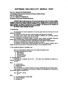
Testing of SRGM Choice and Complexing Procedures To test the developed procedures one of the software testing reports for critical application system was chosen (set of data SYS1 from [1]). A plot of failure intensity function λ(t) alteration in time for software under study is shown in Figure 3. The results of SRGM choice are given below. Analysis of software testing results and their application terms allowed to form the following higher level assumptions: ! I.1 & I.2 & I.3 & I.4; ! II.1.1 & II.2.1.1 & II.2.1.2 & II.2.1.3 & II.3.1. Using binary search tree (Figure 2) we get to a segment of SRGM groups corresponding to NHPP and Hyperexponential models. Having no information of the character of defects we cannot apply Hyperexponential SRGM. Among NHPP SRGM we choose Musa model, as this one permits operating processor time to execute software (Assumption IV.2.3). Thus, we have choice option 1а – SRGM choice from a fixed plurality. Define the form for software failure intensity function. According to IPM for Musa SRGM (Table 1) we have the following input parameters: time (t) and two constants (α, β). As recommended in [7] the model constants would be: 1 α = М 0, β = , М 0 ∗ T0 where М0 – expected number of software failures; Т0 – mean time between failures at the beginning of tests. Thus, for Musa model the failure intensity function is calculated from expression: 1 λ (t ) = exp[ − t /( М 0 T 0 )]. T0

(1)

Usually model parameters in such cases are found by least squares method (LSM) [1, 3]. In order to estimate accuracy of SRGM choice and complexing method compare the accuracy of estimates obtained by this method and LSM.


9

Let us determine the parameters of Musa SRGM. Mean time between failures of software at the beginning of tests increases in the process of program testing and operation. Therefore, it is proposed to select as a period for determination of Т0 in [7] t = 0.1T (T – time of supposed testing). Testing period for software under study was set to be 100000 seconds ≈ 28 hours. From testing protocol [1] we define Т0 (10000 с) = 204 с. The second model parameter, М0 – expected number of failures in software we define by mean arithmetic criterion: S

∑ (λi actual (t ) − λi MusaSRGM (t )) = 0,

(2)

i =1

where S –number of time intervals for which failures intensity was determined. As a result we got an estimate of М0 = 156. According to recommendations in [7] this value may be also taken for the number of expected defects in software. Is should be noted that from test results cited in [1], the total number of defects detected at the testing В = 136. Thus, using chosen SRGM we obtained a sufficiently accurate and verified estimate for one of the most important software reliability measure (relative error less than 15%). A plot of failure intensity obtained with Musa SRGM is given in Figure 5. Further we perform modeling of failure intensity function λ(t) using LSM. For regression equation we take an exponential function of similar form to that in Musa SRGM: λ ( t ) = n exp( − mt ). (3) To define parameters of equation (3) we take the whole set of data on software testing [1], i.e. obtain a degree of accuracy as large as possible in LSM application. The data area being narrowed accuracy of LSM estimate will diminish. To define parameters of LSM function (3) a system of equations must be solved S S  S 2 m t + n t − t ln λ ( t ) = 0 ∑ ∑ ∑  i = 1 i =1 i =1 (4) .  S S  m ∑ t + S ln n − ∑ ln λ ( t ) = 0  i = 1 i =1 After solution of system (4) the following parameters of equation (3) were obtained: m = 0.00002; n = 0.00223. Failure intensity function plots with LSM obtained equation are shown in Figure 3. Comparative analysis of those plots shows that the failure intensity function plot obtained after Musa SRGM better reflects the trends in actual variation of failure intensity function. As to numerical value of criterion (2), for model (3) we have S

∑(λi actual(t ) − λi MusaSRGM(t)) = 0.04. i =1

Thus, a higher accuracy and validity in determination of failure intensity function in this case is attained by proposed method of assumptions matrix analysis (AMA-method). Besides, for two models used multiple determination coefficients were found. Their values made: for Musa SRGM R2 = 0.933187, for LSM R2 = 0.24998, which is also indicative of better quality of λ(t) plot selection performed by AMA-method. The estimate of anticipated number of software failures (corresponding to anticipated number of software defects) as obtained from comparison of expressions (1) and (3) made M 0 = 1 /(т ∗ n) = 112 . Thus, a more accurate estimation of the number of program defects М0 in this case was also obtained using AMA-method. The approbation of the complexing technique was executed for the onboard real-time control system software. The value of output measure (the total number of software faults before beginning of testing) of a parametric reliability model (Halstead model) was taken as SRGM input parameter. The reliability assessment obtained with the help of complexing technique (Halstead and Musa-Okumoto models) gave coincidence with experimental results for 90 per cent of time intervals.


10

λ , 1/second 0,014

actual failure intensity function Musa SRGM

0,012

LSM 0,01

0,008

0,006

0,004

0,002

t, second 0 0

10000

20000

30000

40000

50000

60000

70000

80000

90000

100000

Figure 3. Prediction of software failure intensity using Musa model and least squares method

Features of AMA-Method Using for Reliability Assessment of Software with Predeveloped Components I&C System SW, including software for critical application, consists of the different software components. Some from these components are specialized, i.e. developed specially for the given system (for example, drivers of special-purpose hardware, application software etc.). Other components are predeveloped commercial and specialized software (for example, some application software, operational systems etc.), including COTS-software. The features of application of the offered method for such software (first developed, predeveloped, COTS-software) are analysed in the Table 2. Thus, the proposed technique may be applied for reliability assessment of separate software components, and then for assessment of the multicomponent software as a whole. Table 2. Features of AMA- method application for multicomponent software reliability assessment Analyzed features Exploitation data

First developed software Absent

Software reliability

Reliability is unconfirmed

Necessity of SRGM correction (correction of parameters values)

The model must be chosen taking into account testing data

Features of AMAmethod application

The AMA-method may be used for SRGM choice and reliability assessment

Type of software components Predeveloped software Exist Reliability may be insufficient or unconfirmed The correction may be required (taking into account exploitation data and features of usage of this component in new system) The AMA-method may be used for a reliability reassessment (choice of other SRGM or correction of values of parameters)

COTS-software Exist High reliability The correction is not required The AMA-method is not used


11

Conclusion The proposed method is aimed not to find a universal model of software reliability, but to find a universal method of model synthesis (choice, complexing, fitting). SRGM database must be supplemented and qualified with due consideration of system applications for which software is developed. Joint usage of assumptions matrices and models compatibility analysis permits a purposeful process of SRGM choice. This method is applied in practice for reliability evaluation of an onboard computer-based control system and allowed to improve evaluation accuracy. Usage of the AMA-method for reliability assessment of a multicomponent software containing first developed software components, predeveloped software and COTS-software, is performed in two step: at the first step this technique is applied to choice of SRGM for separate software components, at the second step the generalized software reliability model is composed. This task still requires an additional research. The tools based on proposed technique are developed for decision of these problems [8]. This tools will be joined into the development support system consisting of SRGM database, software defects database, and means of testing, choice and verification of software reliability models.

References [1] Lyu M.R., editor (1996). Handbook of Software Reliability Engineering, McGraw-Hill Company, USA. [2] Musa J.D. and Okumoto K. (1993). Software Reliability Models: Concepts, Classification, Comparisons and Practice. Electronic Systems Effectiveness and Life Cycle Costing, Skvirzynski J.K. (ed.), NATO ASI Series, F3, Springer-Verlag, Heidelberg, 395-424. [3] Polonnikov R.I. and Nikandrov A.V. (1992). Software Reliability Assessment Methods, Polytechnic, San-Petersburg. (Russia). [4] Kharchenko V.S., Sklyar V.V., Vilkomir S.A. (2000). Models Fitting of Software Reliability Assessment for Critical Application Systems. Control Systems and Machines 3, 59-69. (Ukraine). [5] Nikora A. P. and Lyu M. R. (1995). An experiment in determining software reliability model applicability. Proceedings of the 6th International Symposium on Software Reliability Engineering, 304-313. [6] Everett W., Keene S., Nikora A. (1998). Applying Software Reliability Engineering in the 1990s. IEEE Transactions on Reliability 47, 372-378. [7] Musa J.D. (1980). The Measurement and Management of Software Reliability. Proceedings of the IEEE 68:9, 1131-1143. [8] Vilkomir S.A., Kharchenko V.S., Ponomaryev A.I., Gorda A.A. (1999). The System Safety Assessment by the Use of Programming Tools during the Licensing Process. Proceedings of the 17th International System Safety Conference, Orlando, 222 - 227.