the quantum NLS hamiltonians are conserved quantities in these models. ... insight will give us a reasonably simple method for constructing these charges.
hep-th/9210029 IASSNS-HEP-92/57
arXiv:hep-th/9210029v1 6 Oct 1992
Aug 1992
The Nonlinear Schr¨ odinger Equation and Conserved Quantities in the Deformed Parafermion and SL(2,R)/U(1) Coset Models
Jeremy Schiff Institute For Advanced Study Olden Lane, Princeton, NJ 08540
Abstract The relationship between the nonlinear Schr¨odinger hierarchy and the parafermion and SL(2,R)/U(1) coset models, analogous to the relationship between the KdV hierarchy and the minimal models, is explained. To do this I first present an in depth study of a series of integrable hierarchies related to NLS, and write down an action from which any of these hierarchies, and the associated second Poisson bracket structures, can be obtained. In quantizing the free part of this action we find many features in common with the bosonized parafermion and SL(2,R)/U(1) models, and particularly it is clear that the quantum NLS hamiltonians are conserved quantities in these models. The first few quantum NLS hamiltonians are constructed.
1. Introduction It is often stated that there are deep connections between conformal field theories and integrable partial differential equations in 1 + 1 dimensions. The most cited pieces of evidence for this are (1) that the second Poisson bracket structures associated with equations of KdV type are classical limits of the conformal algebras [1] and (2) that the integrals of motion that exist in certain perturbed conformal field theories are quantum analogs of the conserved quantities (“hamiltonians”) of certain integrable PDEs [2]. As has been appreciated in some of the literature (see for example [3]), these two statements are really the same in origin. Most conformal field theories studied to date are themselves integrable, in the sense that in the enveloping algebra of the chiral algebra there exist an infinite number of algebraically independent commuting quantities, and that in some sense which we cannot currently define well, the number of these “integrals of motion ” is half the total number of degrees of freedom of the system*. Given an integrable conformal field theory we can perturb by adding a hamiltonian which is a sum of the conserved quantities; this will give a new theory which is still integrable, having the same conserved quantities. In the context of quantum field theory we are only really interested in relevant, Lorentz invariant perturbations, i.e. adding to the action (`a la Zamolodchikov [2]) integrals of primary fields with dimension less than two. This is in fact mathematically convenient; it seems (but has certainly not been proven) that in general in the conformal field theory there is not a unique way to choose the conserved quantities, but the requirement that the set we choose should include a particular physical hamiltonian pins down the set uniquely. Assuming now that the chiral algebra has some identifiable classical limit, it is quite clear that associated with any integrable conformal field theory and choice of the set of conserved quantities there will be a classical hierarchy of KdV type, with Poisson bracket algebra the classical limit of the chiral algebra, and with hamiltonians the classical limits of the quantum hamiltonians. What might seem surprising is that this construction also seems to work in reverse, that is, all known classical hierarchies of KdV type seem to arise from the classical limit of some conformal field theory. To understand this we need a procedure to obtain a conformal field theory from a classical hierarchy (from the Poisson bracket algebra of the * I thank E.Witten for persuading me that generic conformal field theories are probably not integrable. In any conformal field theory there will be an infinite number of integrals of motion, just by virtue of the fact that the enveloping algebra of the chiral algebra contains the Virasoro algebra. The question is whether there are a sufficiently large number of them. 1
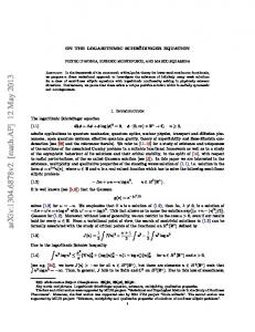
hierarchy we can presumably guess what the chiral algebra of the corresponding theory is, but this is not sufficient). In [4] I described how to construct an action that gave (for the correct choice of parameters) an arbitrary equation in the KdV hierarchy as equation of motion**; this action consisted of a “free” part and a sum of terms proportional to the KdV hamiltonians. I then showed that in quantizing the theory described by the “free” action, with a suitable choice of the coupling constant, we are led to the Feigin-Fuchs description of the (holomorphic sector of the) minimal models, and it becomes clear why the quantum KdV hamiltonians are the conserved quantities associated with the Φ(1,3) perturbation of minimal models [2]. It is obviously of interest to find generalizations of [4], that is to find actions for other integrable hierarchies, and thereby hopefully reveal the underlying conformal field theories; this paper is devoted to doing just this for the case of the non-linear Schr¨odinger (NLS) hierarchy. We will see that the NLS hierarchy is related to the parafermion and SL(2, R)/U (1) coset models, and that the quantum NLS hamiltonians give us give conserved quantities of these models and their deformations. Our classical insight will give us a reasonably simple method for constructing these charges. The action construction for the KdV hierarchy exploited the “quasi-hamiltonian” (or “antiplectic”) formalism for the KdV hierarchy studied by Wilson [6] (see also [7]), and we need an analog of this for the NLS hierarchy. The bulk of this paper (sections 2 and 3a) is devoted to an understanding of the NLS hierarchy and related hierarchies, including the two “Ur-NLS” hierarchies. We establish that the NLS hierarchy is just one in a large tower of hierarchies related by Miura maps; the first non-trivial equations of the ten hierarchies we will have reason to consider, and the principal Miura maps between them, are given in figure 1. Any equation in any of these hierarchies can be obtained by varying a single action with respect to appropriate fields. I hope that the developments in sections 2 and 3a will be of interest beyond the current conformal field theoretic application, and no knowledge of conformal field theory is necessary to read them. I note that certain hierarchies in the NLS tower have been of some interest recently in the context of matrix models [8]. The detailed contents of sections 2 and 3a are as follows: in 2a I introduce the NLS hierarchy and its hamiltonian structures; in 2b I examine four related hierarchies essentially obtained from the standard gauge equivalence class of the NLS hierarchy; in 2c I present the two Ur-NLS hierarchies; in 2d I display the diverse symmetries of the Ur-NLS quasi** Since writing [4] I have been informed that this action is actually well-known, see for example [5]; but in the literature I only see it used as an action for the MKdV hierarchy, and in [4] crucial information is gained by understanding how it serves as an action for the KdV hierarchy too. 2
hamiltonian structures, and use them to gain some insight into the numerous hierarchies in the NLS tower; in 2e I discuss the Toda flows associated with NLS; finally in 3a I introduce three more hierarchies and give the NLS action. The reader is advised to keep figure 1 handy throughout these sections. The remainder of this paper is devoted to finding the conformal field theory related to NLS, and exploiting our understanding of the classical limit of this conformal field theory. In section 3b I explain how the free part of the NLS action is actually related to two different conformal field theories; one of these is of little interest for reasons we shall see, but the other is (depending on the value of the coupling constant) either a parafermion or a SL(2, R)/U (1) coset model, and I show that the quantum NLS hamiltonians are conserved quantities of suitable deformations of these models. In section 3c I point out how the free part of the NLS action is apparently related to a gauged WZW model. This should come as no surprise. Most, if not all, known integrable hierarchies are of Drinfeld-Sokolov type [9] or its generalizations [10]. The second Poisson bracket structures of these hierarchies are all reductions of a Kac-Moody algebra and hence we can construct an associated gauged WZW model as a candidate associated conformal field theory. Finally in section 3d I construct the first few quantum NLS hamiltonians; the results we find are in accord with both the work of Fateev on deformed parafermionic models [11] and the work of Bakas and Kiritsis on conserved quantities in the SL(2, R)/U (1) coset models [12]. Despite work in the literature on both the classical limit of the nonlocal parafermion algebra (which is the second hamiltonian structure of NLS) and integrable deformations of the parafermion models, the relationship of parafermions with NLS seems not to have been observed before. One final comment is in order in this introduction. In [13] a quantization of the NLS hierarchy was proposed along the lines of the quantizations of the MKdV and KdV hierarchies of Sasaki and Yamanaka [14]. Unfortunately in this work the first Poisson bracket of the NLS hierarchy was quantized, and so it is not directly relevant for our work in section 3d where we need quantum NLS hamiltonians with respect to the second Poisson bracket (from work on the quantum KdV equation we do not expect the bihamiltonian structure to survive quantization). But the success of [13] is definitely a positive sign for us. 2. Understanding the Hierarchies related to NLS Throughout this paper I will use the title “the NLS equation” to refer to the coupled system of equations
ψt = ψxx − 2ψ 2 ψ¯
ψ¯t = −ψ¯xx + 2ψ¯2 ψ 3
(2.1)
Here ψ, ψ¯ are independent real fields and x and t are real coordinates. The more usual form of the nonlinear Schr¨odinger equation is obtained by considering (2.1) for t pure imaginary, ψ complex, and ψ¯ the complex conjugate of ψ (then the two equations in (2.1) become complex conjugates of each other). 2a. The bihamiltonian structure of (2.1) and the NLS hierarchy Magri [15] showed that (2.1) has a bihamiltonian structure. The first hamiltonian structure is local, with Poisson brackets � � � � ¯ {ψ(x), ψ(y)} {ψ(x), ψ(y)} 0 −1 = δ(x − y) (2.2) ¯ ¯ ¯ {ψ(x), ψ(y)} {ψ(x), ψ(y)} 1 0 R and hamiltonian H4 = dx (ψx ψ¯x +ψ 2 ψ¯2 ). The second hamiltonian structure is non-local,
with brackets � � � � ¯ {ψ(x), ψ(y)} {ψ(x), ψ(y)} 2ψ∂x−1 ψ ∂x − 2ψ∂x−1 ψ¯ = δ(x − y) (2.3) ¯ ¯ ¯ ¯ −1 ψ ¯ −1 ψ¯ {ψ(x), ψ(y)} {ψ(x), ψ(y)} ∂x − 2ψ∂ 2ψ∂ x x R ¯ x . In (2.3) the matrix on the RHS is evaluated at x, and hamiltonian H3 = dx ψψ Rx Rx and the operator ∂x−1 are defined by ∂x−1 f (x) = 21 ( 0 dx′ f (x′ ) + 2π dx′ f (x′ )), so that R 2π R 2π −1 f2 (x)∂x−1 f1 (x) (the range of x throughout this paper is taken f (x)∂ f (x) = − 1 2 x 0 0 to be [0, 2π]). An infinite number of conserved quantities for the NLS equation are defined by the recursion relation δHn+1 δψ δHn+1 ¯ δψ
!
=
�
¯ −1 ψ ∂x − 2ψ∂ x −2ψ∂x−1 ψ
¯ −1 ψ¯ 2ψ∂ x −∂x + 2ψ∂x−1 ψ¯
� � δHn � δψ δHn ¯ δψ
(2.4)
R ¯ which generates H3 ,H4 as given The recursion is started by setting H2 = − dx ψ ψ, above. The infinite number of conserved quantities generate higher equations in the NLS hierarchy, in the usual fashion. An important point about the Poisson bracket algebra (2.3), which underlies much of what we will do later, was pointed out in [16]; the algebra (2.3) is precisely the Dirac reduction [17] of the SL(2) Kac-Moody algebra under the constraint that the diagonal current is set to zero. 2b. The gauge equivalence class of the NLS equation The NLS equation is a representative of a whole class of integrable evolution equations whose general form is dt = −2φx − (ef )x
et = exx + 4e(φ + d2 ) + 2edx + 4dex
ft = −fxx − 4f (φ + d2 ) + 2f dx + 4dfx 4
(2.5)
This set of equations emerges naturally in the context of reductions of the self-dual YangMills equations; see for example [18]. Equations (2.5) describe the evolutions of functions d, e, f in terms of d, e, f and some auxiliary field φ. The presence of φ allows us to choose some combination of d, e, f that we set to zero (this is called a “gauge choice”), only we then have to adjust φ so that the time derivative of our constraint is zero. This freedom arises because for an arbitrary function α, the replacements d → d + αx /α e → eα−2
f → f α2
(2.6)
φ → φ − αt /2α map solutions of (2.5) to solutions. The NLS equation (2.1) is (2.5) with d = 0, φ = − 12 ef ¯ Note that setting d = 0 in (2.5) does not uniquely determine φ, so (and e = ψ, f = ψ). this is an incomplete gauge fixing; looking at (2.6), we see that this corresponds to the invariance of the (2.1) under ψ → α−2 ψ, ψ¯ → α2 ψ¯ where α is constant. Possible complete
gauge fixings include
1. e = 1, d = A, f = B (φ = −d2 − 12 dx ). The equations are At = Axx + (2A2 − B)x Bt = −Bxx + (4AB)x
(2.7)
A solution of (2.1) gives a solution of (2.7) via A = ψx /2ψ B = ψ ψ¯ 2. f = 1, d = C, e = D (φ = −d2 + 21 dx ). The equations are Ct = −Cxx + (2C 2 − D)x Dt = Dxx + (4CD)x
(2.8)
(2.9)
A solution of (2.1) gives a solution of (2.9) via C = −ψ¯x /2ψ¯
D = ψ ψ¯
(2.10)
There is an obvious invertible map from the solutions of (2.7) to those of (2.9); set C = −A, D = B and let t → −t. But from the gauge transformation relations we get another 5
invertible map not involving change of coordinates C = A − Bx /2B
(2.11)
D=B
Equations (2.7) and (2.9) are thus equivalent, and in the sequel we will just use (2.7). The bihamiltonian structure of the NLS equation (2.1) induces a local bihamiltonian structure for (2.7), the Poisson brackets being � � � � {A(x), A(y)} {A(x), B(y)} 0 ∂x 1 = −2 δ(x − y) (2.12) ∂x 0 {B(x), A(y)} {B(x), B(y)} �
�
� ∂x (∂x + 2A) = δ(x − y) (2.13) 2(∂x B + B∂x ) R (induced by (2.2) and (2.3) respectively). The hamiltonian is H4 = 2 dx (ABx − 2A2 B + R 1 2 B ) for the brackets (2.12) and H = 2 dx AB for the brackets (2.13). The recursion 3 2 relation for the conserved quantities of equation (2.7) (which reduce to those of the NLS {A(x), A(y)} {A(x), B(y)} {B(x), A(y)} {B(x), B(y)}
1 2
�
−∂x −(∂x − 2A)∂x
equation via the substitution (2.8)) is � δHn+1 � δA δHn+1 δB
=
�
∂x − 2∂x−1 A∂x 1
−2(B + ∂x−1 B∂x ) −(∂x + 2A)
� � δHn � δA δHn δB
(2.14)
R R and H2 = − dx B, H1 = − dx A. The A, B hierarchy is an instance of the Broer-Kaup hierarchy studied in [19]. The relationship between equations (2.1) and (2.7) is somewhat analogous to the relationship between the modified KdV and KdV equations. I therefore propose for (2.7) the name the unmodified NLS (M−1 NLS) equation. One other incomplete gauge fixing of the system (2.5) is important. Requiring 2d − e + f = 0, we can take φ = − 1 (ex + fx + (e − f )2 ). Writing e = j, f = ¯j we obtain the 4
equations
jt = (jx + j 2 − 2j ¯j)x
¯jt = (−¯jx − ¯j 2 + 2j ¯j)x
(2.15)
These equations appeared in [20]. Since both (2.1) and (2.15) are incomplete gauge fixings, there is no explicit Miura map between them, but from the gauge transformation laws (2.6) it can be seen that a solution of (2.1) can be found from a solution of (2.15) by quadratures. Solutions of (2.15) generate solutions of (2.7) directly, however, via the map A = 21 (j − ¯j + jx /j)
B = j ¯j
6
(2.16)
For want of a better name I will call (2.15) the NLS2 equation. In the “tower” of equations we are building around the NLS equation, the NLS2 equation is in three ways more analogous to the MKdV equation than the original NLS equation: 1. Whereas for NLS the first bracket structure was local and the second non-local, for NLS2 the first bracket structure is non-local and the second local; explicitly they are [20] � � {j(x), j(y)} {j(x), ¯j(y)} = {¯j(x), j(y)} {¯j(x), ¯j(y)} �
j(∂x + j + ¯j)−1 + (∂x − j − ¯j)−1 j 1 − ¯j(∂x + j + ¯j)−1 + (∂x − j − ¯j)−1 j �
−1 + j(∂x + j + ¯j)−1 − (∂x − j − ¯j)−1 ¯j −¯j(∂x + j + ¯j)−1 − (∂x − j − ¯j)−1 ¯j
{j(x), j(y)} {j(x), ¯j(y)} {¯j(x), j(y)} {¯j(x), ¯j(y)}
�
=
�
0 ∂x
∂x 0
�
δ(x − y)
�
δ(x−y)
(2.17a) (2.17b)
2. The right hand sides of (2.15) are total x-derivatives, unlike those of (2.1), so from ¯ by j = hx , (2.15) we can naturally define a “potential” NLS equation; introducing h, h ¯ satisfy ¯ x we see that if h, h ¯j = h ¯x ht = hxx + h2x − 2hx h
¯ t = −h ¯ xx − h ¯ 2 + 2hx h ¯x h x
(2.18)
then j, ¯j satisfy (2.15). In fact solutions of (2.18) also give rise to solutions of (2.1), but the Miura map is less obvious: ¯ ψ = eh−h hx (2.19) ¯ ¯ ψ¯ = e−(h−h) h x 3. As noted above, the NLS equation has a very obvious invariance under ψ → α−2 ψ, ¯ which is effectively “modded out” when we pass to the M−1 NLS equation. The ψ¯ → α2 ψ,
corresponding invariance of NLS2 is hidden, like that of the MKdV equation [6]. For completeness I note that the recursion operator for the NLS2 equation is � � ∂x + ∂x−1 jx + ¯j − j ∂x−1¯jx − 2¯j (2.20) −∂x−1 jx + 2j −∂x − ∂x−1 ¯jx + ¯j − j and the first few conserved quantities are Z 1 H1 = − 2 dx (j − ¯j) Z H2 = − dx j ¯j Z H3 = dx (¯jjx + (j − ¯j)j ¯j) 7
(2.21)
Note also that the NLS2 equation (2.15) reduces to Burger’s equation [21] on setting ¯j = 0. So far in this section I have described the NLS, M−1 NLS, and NLS2 equations, all of which emerge from the scheme (2.5), and the potential NLS equation, which has an “obvious” relationship to NLS2. There is one more equation that has an “obvious” relationship to NLS2; given a solution of NLS2, construct U, V by U = j − ¯j
(2.22)
V = (j + ¯j)x − 21 (j + ¯j)2 Then U, V satisfy Ut = Vx + 3U Ux
(2.23)
Vt = Uxxx + Vx U + 2Ux V
I will call this the M−1 NLS2 equation. M−1 NLS2 inherits local bihamiltonian structure from NLS2, with brackets � � � {U (x), U (y)} {U (x), V (y)} 0 =2 {V (x), U (y)} {V (x), V (y)} ∂x �
{U (x), U (y)} {U (x), V (y)} {V (x), U (y)} {V (x), V (y)}
�
�
= −2
∂x 0
∂x −(∂x U + U ∂x )
�
0 3 ∂x + V ∂ x + ∂x V
δ(x − y)
(2.24)
�
(2.25)
δ(x − y)
R The respective hamiltonians are H4 = 41 dx (V 2 + 3U 2 V + 54 U 4 − Ux2 ) and H3 = R − 21 dx (U V + 21 U 3 ). Further hamiltonians can be defined by the recursion relation � δHn+1 � δU δHn+1 δV
and H1 = − 12
R
=−
dx U , H2 =
1 2
∂x2 + V + ∂x−1 V ∂x 0
� � δHn �
�
U + ∂x−1 U ∂x 1
R
dx (V + 21 U 2 ). It is not clear that the hamiltonians defined
δU δHn δV
(2.26)
here coincide with those we have used previously, but it turns out this is indeed the case (i.e. Hn [U, V ] and Hn [A, B] agree when written as functionals of j, ¯j). Now in some sense M−1 NLS and M−1 NLS2 are not really distinct. If U, V satisfy M−1 NLS2 (2.23) then A˜ = 12 U (2.27) ˜ = 1 (−2V + 2Ux − U 2 ) B 4 satisfy M−1 NLS (2.7). Furthermore (2.27) maps the second hamiltonian structure (2.25) of M−1 NLS2 to that (2.13) of M−1 NLS, and the first hamiltonian structure (2.24) is taken to minus (2.12). So although because of this minus sign the map (2.27) is not strictly a Miura map of the M−1 NLS2 hierarchy to the M−1 NLS hierarchy, we might wish to consider M−1 NLS and M−1 NLS2 as equivalent. But remarkably the composite Miura map from 8
NLS2 to M−1 NLS defined by (2.22) and (2.27) is not the same as the direct map (2.16). So if we were to regard M−1 NLS and M−1 NLS2 as the same, each time we wished to use a Miura map to pass from NLS2 to the single “unmodified” equation, we would have to specify which map we were using. This is potentially confusing. So we will opt, in the rest of this paper, to treat M−1 NLS and M−1 NLS2 as distinct; thus all our Miura maps are genuine maps of hierarchies, and different Miura maps go to different equations. Still, the existence of two distinct Miura maps from the NLS2 equation to the M−1 NLS equation is a most remarkable result. To summarize section 2b: using the scheme (2.5) we have obtained five of the equations indicated in figure 1. I should point out here that (2.5) is really only a restricted set of the equations in the gauge equivalence class of the NLS equation. For further details see [18]. 2c. Antiplectic formalism for the NLS equation From the work of Wilson [6] we recognize the need to find an “Ur-NLS” hierarchy; this should generate solutions of the potential NLS hierarchy (2.18) via a Miura map (and hence will give us solutions of the NLS, NLS2, M−1 NLS, and M−1 NLS2 hierarchies), and it should have an inverse-local bihamiltonian form. We expect the two inverse-local hamiltonian structures to induce the second and third Poisson bracket structures of the various equations of section 2b. The third Poisson bracket structures are obtained by letting the recursion operators act (from the right) on the matrices appearing in the second bracket structures; I will just give the explicit form of the third bracket structure for the NLS2 equation, which is of particular interest since it is local [20]: �
{j(x), j(y)} {j(x), ¯j(y)} {¯j(x), j(y)} {¯j(x), ¯j(y)}
�
=
�
∂x j + j∂x 2 ∂x + ∂x ¯j − j∂x
−∂x2 − ∂x j + ¯j∂x −(∂x¯j + ¯j∂x )
�
δ(x − y)
(2.28)
It turns out that there are actually two Ur-NLS hierarchies (related in the same way as M NLS and M−1 NLS2). I do not plan to give a full derivation here of these hierarchies, since much will be obvious after reading sections 2d and 3a below; here I will just give the −1
equations, their two Poisson bracket structures and the associated local symplectic forms, and the Miura maps to the potential NLS hierarchy. I will call the following equation the Ur-NLS1 equation: Tt = Txx + 2Tx Sx 2Sx Txx + 3Sx2 − Sxx St = Tx It is a straightforward but tedious business to check the following results: 9
(2.29)
1. If S, T satisfy Ur-NLS1 then h=S
(2.30)
¯ = −S + ln(Sx T −1 ) h x satisfy the potential NLS equation. 2. The bracket structure � � � {S(x), S(y)} {S(x), T (y)} 0 = −1 {T (x), S(y)} {T (x), T (y)} ∂x Tx ∂x−1
−∂x−1 Tx ∂x−1 2∂x−1 Tx ∂x−1 Tx ∂x−1
�
δ(x − y)
(2.31)
induces, via the various Miura maps given, the second hamiltonian structures of the NLS, NLS2, M−1 NLS and M−1 NLS2 equations. The inverse of the matrix on the right hand side of (2.31) is � � 2∂x ∂x Tx−1 ∂x (2.32) −∂x Tx−1 ∂x 0 which is a local operator, associated with the symplectic form Z Ω2 = 2 dx δ(S + ln Tx ) ∧ δSx 3. The bracket structure � � � {S(x), S(y)} {S(x), T (y)} Sx ∂x−1 + ∂x−1 Sx =− {T (x), S(y)} {T (x), T (y)} Tx ∂x−1
∂x−1 Tx 0
(2.33)
�
δ(x − y)
(2.34)
induces, via the various Miura maps given, the third hamiltonian structures of the NLS, NLS2, M−1 NLS and M−1 NLS2 equations. The inverse of the matrix on the right hand side of (2.34) is � � 0 −∂x Tx−1 (2.35) −Tx−1 ∂x ∂x Sx Tx−2 + Sx Tx−2 ∂x which is a local operator, associated with the symplectic form � � Z Sx Ω3 = −2 dx δT ∧ δ Tx
(2.36)
I will call the following equation the Ur-NLS2 equation: τt = −τxx − 2τx σx 2σx τxx σt = σxx − 3σx2 − τx This is (2.29) with t → −t. We check: 10
(2.37)
1. If σ, τ satisfy Ur-NLS2 then h = −σ
(2.38)
¯ = σ + ln τx h
satisfy the potential NLS equation. 2. The � bracket structure � � {σ(x), σ(y)} {σ(x), τ (y)} 0 = −1 {τ (x), σ(y)} {τ (x), τ (y)} ∂x τx ∂x−1
−∂x−1 τx ∂x−1 2∂x−1 τx ∂x−1 τx ∂x−1
�
δ(x − y)
(2.39)
induces, via the various Miura maps given, the second hamiltonian structures of the NLS, NLS2, M−1 NLS and M−1 NLS2 equations. Comparing with (2.31) we see that the inverse of the matrix on the right hand side of (2.39) is a local operator, associated with the symplectic form Z ˜ 2 = 2 dx δ(σ + ln τx ) ∧ δσx Ω (2.40) 3. The �bracket structure � � {σ(x), σ(y)} {σ(x), τ (y)} σx ∂x−1 + ∂x−1 σx = {τ (x), σ(y)} {τ (x), τ (y)} τx ∂x−1
∂x−1 τx 0
�
δ(x − y)
(2.41)
induces, via the various Miura maps given, the third hamiltonian structures of the NLS, NLS2, M−1 NLS and M−1 NLS2 equations. Comparing with (2.34), the inverse of the matrix on the right hand side of (2.41) is a local operator, associated with the symplectic form ˜3 = 2 Ω
Z
dx δτ ∧ δ
�
σx τx
�
(2.42)
As mentioned above we see that the relationship between the two Ur-NLS hierarchies is the same as that between the two M−1 NLS hierarchies. The two Ur-NLS equations are related by a t → −t transformation, the second bracket structures are identical, and the third bracket structures are identical up to an overall minus sign. Again though, because of these sign differences, and more importantly because of the different forms of the Miura maps (2.30) and (2.38), we will regard Ur-NLS1 and Ur-NLS2 as distinct. In sections 2d and 3 we will see how Ur-NLS1 is related to M−1 NLS and how Ur-NLS2 is related to M−1 NLS2, thus explaining why I have chosen to number the two equations in this way. 2d. Group-theoretical origin of the antiplectic formalism The symplectic forms Ω2 , Ω3 that appeared in section 2c in the context of the Ur-NLS1 equation, have a natural group theoretical origin. Consider an SL(2) matrix valued function g(x) such that the diagonal component of g −1 gx vanishes. Choosing a Gauss decomposition for g �� � � � � −S 1 0 1 T e 0 (2.43) g= φ 1 0 1 0 eS 11
where S, T, φ are functions of x, the requirement that the diagonal component of g −1 gx vanishes can be solved to give Sx e−2S (2.44) φ= Tx and we then have g=
�
e−S (1 + T Sx Tx−1 ) Sx Tx−1 e−S
T eS eS
�
With this choice of g it can be checked that Z Ω2 = − dx T r[δgg −1 ∧ ∂x (δgg −1)] � �� � �� Z 1 1 0 −1 −1 Ω3 = dx T r g δg ∧ , g δg 0 −1 2
(2.45)
(2.46)
The first of these formulas is an analogue of the one given for the KdV equation in [6]. For the KdV equation the SL(2) matrix g has to satisfy the constraint that the (12) entry of g −1 gx is 1; this constraint can be solved to give all the components of g in terms of two functions, but it turns out that the form Ω2 is independent of one of these. The resulting symplectic form is the form associated with the second hamiltonian structure of the UrKdV equation. The symplectic form associated with the third hamiltonian structure of the Ur-KdV equation can also be obtained from a formula to the second one in � similar � 0 0 (2.46); just the matrix appearing should be replaced by [18]. 1 0 Having obtained the formula for Ω2 in (2.46) we can now examine its symmetries, to obtain an “explanation”, in the sense of Wilson, as to why some of the equations in the NLS tower exist. Looking at (2.33) we observe that Ω2 is invariant under S → S + s, T → T + t, where s, t are constants, but from (2.46) we see that it is also invariant under
g → hg where h is a constant SL(2) matrix (and this preserves the constraint that g −1 gx should have vanishing diagonal component). Writing h=
�
a b c d
�
(2.47)
where ad − bc = 1, the corresponding action on S, T is given by eS → (cT + d)eS aT + b T → cT + d
(2.48)
Taking a = d = 1, c = 0 we replicate the translational symmetry in T observed before; the translational symmetry in S is however distinct from the SL(2) invariance. Thus we have 12
in total an SL(2) × R symmetry group, with parameters a, b, c, d, s with ad − bc = 1. Some of the equations in the NLS tower now become clear. In moving from Ur-NLS1 to potential NLS we mod out by just the T translational symmetry; in moving from Ur-NLS1 to NLS we mod out by the full SL(2) symmetry, leaving the non-hidden residual one-parameter symmetry that we have mentioned; in moving from Ur-NLS1 to NLS2 however, we mod out by the S translational symmetry and the subgroup of upper triangular matrices in SL(2), which is not a normal subgroup and hence leaves us with a hidden residual one-parameter symmetry; finally in moving to the M−1 NLS equations we mod out by the full SL(2) × R symmetry. ˜ 2 are identical But what of the Ur-NLS2 and M−1 NLS2 equations? Because Ω2 and Ω ˜ 2 is invariant under translation of σ and an SL(2) action like (2.48). we know that Ω Comparing (2.30) and (2.38) we see that S translation and σ translation are equivalent, but the SL(2) actions on the S, T variables and the σ, τ variables are at least partially ¯ variables are distinct since distinct (by this I mean that their induced actions on the h, h we cannot compare their full actions directly). One way to verify that the two SL(2) actions are distinct is to check that under the S, T SL(2) action A, B are invariant but U, V are not, while under the σ, τ SL(2) action U, V are invariant, but A, B are not. So we are led to the conclusion that the NLS tower really consists of two sub-towers, the first (Ur − NLS1 → PotNLS → NLS or NLS2 → M−1 NLS) related to the symmetry in the S, T variables, and the second (Ur − NLS2 → PotNLS → NLS2 → M−1 NLS2) related to
the symmetry in the σ, τ variables. That these two sub-towers have equations in common may be a coincidence, or may indicate some higher structure, namely the existence of a “M−2 NLS” equation for variables which are invariant under both SL(2) actions, and possibly a corresponding “Ur2 − NLS” equation for variables upon which both SL(2)
actions are manifest. I have been unable to find such a structure to date.
2e. Additional Flows
To complete the picture we have of the NLS system, we need one more ingredient. The NLS hamiltonians form a “complete set”, in the sense that there are no more functionals of A, B (or U, V ) which are integrals of local densities and commute with the Hn , n = 1, 2, 3, ... ¯ given above [13]. However if we are willing to consider integrals of local densities in h, h then there are some additional hamiltonians we should look at; these generate flows that 13
are the analogs of the Liouville and Sine-Gordon flows in KdV theory. Introduce Z ¯ H1 = dx eh+h Z ¯ H2 = dx hx e−(h+h)
(2.49)
H1 ,H2 have simple interpretations. From section 2d there are two one-parameter hidden symmetries of the j, ¯j system (the residual symmetries from the two SL(2) actions that we have not yet removed). H1 and H2 are the generators of these symmetries (H1 comes form the σ, τ SL(2) action, and H2 from the S, T SL(2) action). Hence it is evident that
H1 commutes with Hn when written as a functional of U, V , since it commutes with U and V , and it is evident that H2 commutes with Hn when written as a functional of A, B, since it commutes with A and B. Note that H1 vanishes when we write it in terms of σ, τ , and assume periodic boundary conditions, and H2 similarly vanishes when we write it in terms of S, T . Note that H1 and H2 do not commute with each other. The actual forms of the flows will interest us little in the sequel, but for completeness I will write them down; a hamiltonian µ1 H1 + µ2 H2 generates the flow ¯
¯
hxt = µ1 eh+h − µ2 hx e−(h+h)
(2.50)
¯ ¯ xt = µ1 eh+h¯ + µ2 h ¯ x e−(h+h) h
¯ but H2 generates an interesting We see that H1 generates a Liouville flow (for h + h), integrable flow that I have not seen before in the literature. 3. The NLS Action and Associated Quantum Theories 3a. The NLS action To readers of [4] it will come as no surprise that every equation in the NLS tower can be derived from a single action by varying it with respect to different fields. The action can be written SNLS = k˜
Z
¯t + dxdt hx h
∞ X
n=1
λn
Z
dt Hn +
2 X i=1
µi
Z
dt Hi
(3.1)
˜ λn , µi , n = 1, 2, ..., i = 1, 2, are constants. In particular: the M−1 NLS hierarchy is Here k, obtained by varying SNLS (with µi = 0) with respect to the Ur-NLS1 variables S, T and vice-versa; the M−1 NLS2 hierarchy is obtained by varying SNLS (with µi = 0) with respect to the Ur-NLS2 variables σ, τ and vice-versa; the NLS2 hierarchy and the “additional ¯ flows” (2.50) are obtained by varying SNLS with respect to the PotNLS1 variables h, h; 14
the PotNLS hierarchy is obtained by varying SNLS (with µi = 0) with respect to the NLS2 variables j, ¯j. To obtain the original NLS hierarchy from (3.1) we need to introduce a new set of variables p = T , q = Sx /Tx ; if S, T satisfy the Ur-NLS1 equation then p, q satisfy what we shall call the AuxNLS equation, pt = pxx + 2p2x q qt = −qxx + (2q 2 px )x
(3.2)
A Miura map from the AuxNLS equation to the NLS2 equation is given by j = qpx ¯j = −qpx + qx /q
(3.3)
We can exploit this to vary SNLS (with µi = 0) with respect to p, q to obtain the NLS ¯ hierarchy; similarly we obtain the AuxNLS hierarchy by varying with respect to ψ, ψ. Finally, although it will be of no relevance for the work in the rest of this paper, I have indicated in figure 1 the first equations of two more hierarchies in the NLS tower, the well-known derivative NLS (DNLS) hierarchy [22], and a quintic NLS (QNLS) hierarchy. Solutions of DNLS can be obtained via Miura maps from both the PotNLS and AuxNLS equations, and generate solutions of NLS2. Solutions of QNLS can be obtained via Miura maps from PotNLS, and generate solutions of both NLS and NLS2. All details are in figure 1. The DNLS hierarchy is obtained from the action by varying it with respect to the QNLS variables and vice-versa. Direct verification of everything in the above paragraph is mostly tedious but straightforward. Amongst the harder manipulations is finding the variation of the first term in ¯ (3.1) (which I will call S0 ) with respect to the sets of variables {A, B}, {U, V }, {ψ, ψ}, ˜ {p, q}. S0 is a non-local functional of any of these sets of variables. The {P, Q}, {P˜ , Q}, formulae for the variation are: Z δS0 = dxdt Z = dxdt Z = dxdt Z = dxdt Z = dxdt Z = dxdt
� � � � Tt Sx Tt − St δA + δB 2 Tx Tx � � �� τt τtx δU − δV σt + 2τx 2τx � � (qt − q 2 pt )e−2h δψ + pt e2h δ ψ¯ h i 2h ˜ −2h ˜ e Qt δP + e Pt δQ
h i ˜ −e−2h Qt δ P˜ − e2h Pt δ Q
h i ¯ (e2h ψt − e2h ψ¯t )δp − e−2h ψt δq 15
(3.4)
For illustrative purposes I also give here a formula (which also is quite intricate to obtain) for the variation of the hamiltonian terms of (3.1) with respect to {p, q} (this calculation is required to recover the usual NLS hierarchy from (3.1)); if F is an arbitrary functional of A, B we find δF =
Z
h i ¯ −2h 2h 2h 1 −1 ¯ ¯ ¯ dxdt (ψFA − (ψFB )x )(e δq − e δp) + (( 2 ψ FAx − ψFB )x − ψFA )e δp
where FA , FB
(3.5) denote functional derivatives of F with respect to A, B respectively. Com-
bining (3.5) and the appropriate part of (3.4) it is clear how to vary SNLS with respect to {p, q}; the usual form of the NLS hierarchy is recovered from the resulting equations by ¯ ¯ − ψFψ ), FB = ψ −1 F ¯ . using the results FA = 2∂x−1 (ψF ψ ψ
The other important property of the action SNLS is that the canonical Poisson brack-
ets associated with it [4] coincide with the second hamiltonian structure of the NLS hierarchy (up to an overall constant). These brackets are of course determined purely by S0 , the only part of the action with a time derivative. Thus in the sequel we will be quantizing the NLS hierarchy using its second hamiltonian structure (in contrast to [13] where the first hamiltonian structure is used). 3b. The related conformal field theories Following [4] we would like to relate the term S0 in SNLS to a conformal field theory. In fact two conformal field theories emerge from S0 , essentially because we can treat either the variables S, T or σ, τ as fundamental; the choice here determines the nature of the ¯ that appear in the free action S0 . If we choose S, T as fundamental fields, then fields h, h ¯ satisfy the constraint H2 = 0; if we choose σ, τ as fundamental fields, then h, h ¯ satisfy h, h the constraint H1 = 0. The two different constraints give two very different theories; the well-defined fields in each of the two theories have to commute with the relevant constraint,
so in the theory based on variables S, T well-defined fields are functionals of A, B, and in the theory based on variables σ, τ well-defined fields are functionals of U, V . We can deduce at once that the theory based on variables σ, τ is not going to be very interesting. Looking at (2.25) we see that the variables U, V decouple (at the classical level, but this will remain true at the quantum level). The conformal field theory associated with ˜ consists of a c = 1 scalar field S0 [σ, τ ], for appropriate values of the coupling constant k, and a minimal model. The significance of the NLS hamiltonians in this theory will be that if we perturb the model by adding a term proportional to a suitably quantized version of R dt H2 , then we expect the model to remain integrable, with conserved quantities given by quantum analogs of the NLS hamiltonians. But from the form of H2 it seems that 16
such a perturbation will be of very limited physical interest. So I will not investigate this further. In the theory based on variables S, T , however, we will use H1 as our perturbation,
and this looks more interesting. So we need to quantize S0 with H2 = 0 imposed as a constraint. Defining fields φ1 , φ2 by −i (φ1 − φ2 ) h= √ 2 k+2 ¯ = √−i (φ1 + φ2 ) h 2 k+2
(3.6)
˜ by k˜ = −(k + 2)/2π, we have where k is related to k 1 S0 = 8π
Z
dxdt (φ1x φ1t − φ2x φ2t )
(3.7)
Operators in the theory depend on x, so we can translate them into operators that are holomorphic in one complex variable z in the standard fashion [14] (identifying x with the angular coordinate of the unit circle in the z-plane). The normalization of (3.7) is such that two point functions are given by hφ1 (z)φ1 (w)i = −2 ln(z − w) hφ2 (z)φ2 (w)i = +2 ln(z − w)
(3.8)
We wish to quantize (3.7) subject to a constraint I
dzJ(z) = 0
(3.9)
√ where we will take J(z) = φ2z exp (iφ1 / k + 2) (we can apparently add a total derivative to J without affecting the constraint; this is simply the most compact choice). Looking at [23] or [24], we see already that our theory for integer k has much in common with the bosonized Zk parafermion theory; both are expressed in terms of two bosons, one H with negative signature, and in the parafermion theory dz J(z) is one of the screening
operators (so the states in the theory are characterized by the condition that they are H annihilated by dz J(z), in a certain sense). For k < −2 our theory has the features
of the SL(2, R)−k /U (1) coset model [12]. The analogy continues: classically, we had ¯ A, B all of which commute with H2 ; A has a quotient when four composite fields ψ, ψ, expressed in terms of h, ¯h, so its quantum analog will be difficult to handle, but we would ¯ B all to have sensible quantum analogs (which commute with the constraint). expect ψ, ψ, 17
Alas, assuming we quantize the constraint by a simple normal-ordering of the classical ¯ B expression, it is too much to expect that we might derive the quantum analogs of ψ, ψ, by normal-ordering of the classical expressions. We find we need to modify the classical expressions � � iφ2 −i (φ1x − φ2x ) exp √ ψ= √ 2 k+2 k+2 � � −iφ −i 2 (3.10) (φ1x + φ2x ) exp √ ψ¯ = √ 2 k+2 k+2 1 B= (−φ21x + φ22x ) 4(k + 2) to quantum expressions −i ψ =: √ 2 k+2
r
−i ψ¯ =: √ 2 k+2
r
k+2 φ1x − φ2x k
! !
exp
� �
iφ2 √ k
�
−iφ2 exp √ k � � 1 2i φ1xx : B =: −φ21x + φ22x + √ 4(k + 2) k+2 k+2 φ1x + φ2x k
: �
:
(3.11)
which are (up to normalizations) the usual expressions for ψ1 , ψ1† , T in the bosonized Zk parafermion model [23][24], or ψ±1 , T in the bosonized SL(2, R)−k /U (1) model [12]. Note that (up to overall normalization) the quantum fields ψ, ψ¯ are the only fields of the form : (λφ1x + µφ2x)eiνφ2 : (with λ, µ, ν constants) that commute with the constraint; similarly the improvement we have to make to B in the quantum theory is uniquely dictated. So we have given here a novel approach to the construction of the bosonized parafermionic theory; in the usual approaches [23][24] the discovery of the screening operator : J(z) : is very ad hoc, whereas in our approach it arises very naturally, as the one object transcribed directly from the classical theory to the quantum theory, and used to determine the correct quantized forms of all other operators of interest. At this point it is appropriate to mention that there are features of the Zk parafermion theory which it seems we cannot derive from our classical theory, such as the other screening operators used in [24]. Therefore I have taken care not to call the S0 an action for the parafermion theory, rather I have just described it as related to the parafermion theory (in the specific sense that both the operators in the quantum theory based on S0 and in the parafermion theory have to commute with the constraint (3.9)). What is the quantum analog of the NLS hamiltonians? In the classical theory the NLS hamiltonians were quantities that commuted with both H1 and H2 . So in the quantum 18
theory, the NLS hamiltonians will have to commute with not only the constraint, but also with another operator which is a quantized version of H1 . Here a problem appears; there
is apparently no natural way to specify the quantum analog of H1 . This actually will turn out to be to our advantage; naively quantizing H1 , we would take its quantum analog to be � � Z −iφ1 : (3.12) dx : exp √ k+2 but we will allow ourselves the freedom of generalizing this to � � Z −ilφ1 dx : exp √ : k+2
(3.13)
where l is a constant. Allowing this we see at once that the quantum NLS hamiltonians are the conserved quantities under thermal perturbations of the parafermion models (and similar perturbations of the SL(2, R)/U (1) coset models). In the parafermion theory the significance of requiring operators to commute with the operator (3.12) is that they are conserved quantities under perturbation by the first thermal operator [11]; requiring commutation with the operator (3.13) (for positive integer l) gives us conserved quantities under perturbation by the lth thermal operator. So we see that by allowing the possibility (3.13) we stand the chance to learn more. We will return to the explicit construction of the first few quantum NLS hamiltonians in section 3d; we will see that for l 6= 1 not all the NLS hamiltonians survive the quantization, but for l = 1 it is possible they do. 3c. Understanding S0 Although the form of S0 given in section 3a is obvious to guess, given that we know we want the j, ¯j Poisson bracket structure (2.17b), S0 has a much deeper origin, which in particular will explain the formula for Ω2 in (2.46). Let g(x, t) be an SL(2) valued function, with a Gauss decomposition as in (2.43), and with the diagonal component of g −1 gx vanishing, so (2.44) holds. Then S0 (as a functional of S, T , which is how we are now treating it) is simply the WZW action for g. This can be checked using the formulae of [25] (note that the crucial result we have used, that we need to supplement the action S0 as a functional ¯ with a constraint, was also obtained in [25]). The formula for Ω2 in (2.46) is the of h, h symplectic form associated with the WZW action, pulled back to the space of SL(2) valued functions g(x) with the diagonal component of g −1 gx vanishing. Note that in general if we specify the hamiltonian structure of some model by giving a symplectic form, it is very easy to restrict the model by some constraint; we simply pull back the form. However, if the hamiltonian structure is specified via a set of Poisson brackets, we have to do a Dirac reduction; in our case we have to reduce the SL(2) Kac-Moody algebra, the Poisson 19
bracket algebra of the SL(2) WZW model, by the constraint that the diagonal current vanishes. This gives the original second Poisson bracket structure of the NLS equation, (2.3). We see that from (2.3) we might have directly deduced that an appropriate action for the NLS hierarchy would be the SL(2) WZW model for g with the diagonal component of g −1 gx vanishing, plus a sum of the NLS hamiltonians (the WZW action, being first order in (light-cone) time derivatives, gives no hamiltonian, but determines Poisson brackets). For certain G/H coset models, Park [26] has proposed considering an action SW ZW (mg ). This action is a functional of a G valued function g, and mg is defined so that m−1 g mgx is orthogonal to the Lie algebra of H in the Lie algebra of G. Our S0 is an instance of Park’s action. By a simple path integral manipulation, Park has shown the equivalence of the theory based on his action with the theory based on the usual gauged WZW action for coset models [27]. But as I have said above, some features of the coset model are not immediately apparent from the canonical quantization of the Park action. Clarification of this issue would be interesting. In addition to the relation to the Park action, it would seem that S0 also has a direct relation to the usual gauged WZW action. Bardakci et al. [28] have shown that in the classical G/H gauged WZW model there are certain composite fields that satisfy a “classical parafermion algebra”, i.e. the Dirac reduction of the G Kac-Moody algebra by the constraints that the H currents are set to zero (of course, in the theory defined by Park’s action it is completely clear that there are fields satisfying this algebra). This being the case, we should be able to identify S0 as (maybe a term in) a gauged WZW model. This may help to find the additional information needed for a complete Lagrangian description for the parafermion models; however we will not investigate this here. 3d. The first few quantum NLS hamiltonians We now return to the explicit construction of the first few quantum NLS hamiltonians. R The spin s−1 quantum NLS hamiltonian should have the form dx : Ts : where Ts is some spin s operator constructed out of φ1x , φ2x and their derivatives. Clearly we can freely add to Ts a total derivative, and we also would hope that the quantum NLS hamiltonians share the symmetry of the classical NLS hamiltonians that under φ2 → −φ2 , Ts → (−1)s Ts . The overall normalization of Ts is unimportant for our purposes but we will nevertheless choose not to fix it. Given all this, we should look for the first few T ’s in the form T2 = α1 φ21x + α2 φ22x T3 = β1 φ21x φ2x + β2 φ32x + β3 φ1x φ2xx T4 = γ1 φ41x + γ2 φ21x φ22x + γ3 φ422 + γ4 φ1x φ2x φ2xx + γ5 φ21xx + γ6 φ22xx 20
(3.14)
We require the quantum NLS hamiltonians to commute with the quantum analogs of H1 (which depends on the parameter l) and H2 . Defining Φ1 = φ2x eiµφ Φ2 = e−ilµφ
(3.15)
√ where we have written µ = 1/ k + 2, this means that we need to enforce the following OPEs: X Ψsi,r (z) ∂z Ψsi,0 (z) Ts (z ′ )Φi (z) = + + reg. (3.16) ′ r+1 ′ −z (z − z) z r>0
for i = 1, 2. Here Ψsi,r denote some normal ordered operators whose form is unimportant for us. In general what seems to happen is that the OPE of Ts with Φ1 determines some relations between the coefficients of Ts , and the OPE with Φ2 fixes the remaining
coefficients (up to an overall normalization), and also gives constraints on l. The T2 case is somewhat trivial; we just find we need α2 = −α1 , and any l is permitted. For T3 from the Φ1 OPE we obtain
β2 =
�
� 2µ2 − 1 β1 3
(3.17) 2 2 β3 = (µ − 1)β1 iµ The Φ2 OPE yields the requirement l = 1. So only if we quantize H1 in the naive fashion,
as explained in section 3b, do we obtain a spin 2 conserved quantity. Moving on to T4 we see some of the features I expect to be present in the general case. We find from the Φ1 OPE:
γ3 = (2µ2 − 1)γ1 + (µ2 − 1)γ2 � 2 6(2µ2 − 1)γ1 + (4µ2 − 3)γ2 γ4 = iµ � � � � 1 1 2 γ5 = 2 − 2µ γ1 + − 2 γ2 µ2 µ2 � � 2 � � 2µ 1 1 2 + 1 − 2 γ2 γ6 = 2 2µ − 1 − 2 γ1 + µ 3 µ
(3.18)
4 2 2 (l µ − 1)γ2 ilµ � � 1 2 2 γ5 = 4 3 − l µ − 2 2 γ1 l µ
(3.19)
Thus one coefficient in T4 is not fixed. The Φ2 OPE gives γ4 =
These fix the last coefficient and give a consistency condition for l, which is solved to give l = 1 or l = 2. Note the coefficients in T4 depend on the choice of l; for example for l = 1 we find γ2 = −6γ1 and for l = 2 we find γ2 = 3(2µ2 − 1)γ1 . 21
The scheme of results above is in agreement with the literature. For the Zk parafermion model, spin 2 and 3 conserved quantities in the first thermal perturbation, and a spin 3 conserved quantity in the second thermal perturbation were given in the appendix of [11]. For the SL(2, R)/U (1) coset model spin 2 and spin 3 conserved quantities, corresponding to our results for l = 1, were given in [12]. The simple forms of the coefficients γ3 , ..., γ6 (after setting γ2 = −6γ1 ) seem quite remarkable when compared to the complexity of equations (5.7),(A.1),(A.2),(B.1) in [12], but explicit checks of γ4 and γ5 (which are the two formulae needed to determine l) show the equivalence. We have avoided many of the steps of [12], and indeed lost some information found there, but from the point of view of explicit construction of the charges the method presented here is more efficient. One piece of information we have not obtained is the fact that there is a W −algebra ˆ ∞ (−k) algebra for in all of our models, a Wk algebra for the Zk parafermions and a W the SL(2, R)−k /U (1) models [12]. From [11] we know that for the l = 1 deformation of the Zk parafermion model there should be conserved quantities for all spins which are not zero modulo k. The spin 2 and 3 conserved quantities constructed above seem to exist even for k = 2 and k = 3. They must vanish by the correct choice of certain k-dependent normalization factors, but I cannot at present see a method of fixing the normalizations. The truncation of the parafermionic W −algebra has been studied in depth in [29], from which it seems that the reason the W −currents of spin ≥ k can be ignored in the Zk parafermion model is also a result of correct normalization in their definition, but it is not obvious how the normalization should be chosen. This question needs further study. But for now we have to accept the results from above for the parafermion case with a little caution. Some constraint on the normalization of the quantum NLS hamiltonians is obtained by requiring the correct classical limit, but this is not enough to resolve the ¯ question raised here. The classical limit is obtained by writing everything in terms of h, h via (3.6) and taking k → ∞; the normalizations of the classical NLS hamiltonians can be related by the recursion relation (2.20). For the coset model case there is apparently no problem of the type mentioned above (except possibly for certain rational values of k). The existence of a W∞ type algebra in the SL(2, R)/U (1) coset model seems in fact to be of very limited physical significance (just as the fact that one can build operators satisfying a W∞ type algebra from a single boson is only really a result of interest from the point of view of W∞ algebra representation theory). We have seen how to construct the charges of the theory without mentioning the W −algebra, and we have also one interesting new piece of information from our approach: the conserved charges of the SL(2, R)/U (1) coset model studied in [12] (see also [30]) are only one particular choice for the conserved charges of the model, those appropriate to 22
the first thermal perturbation. There are other infinite sets as well, appropriate to other perturbations. Whether any of these sets have physical significance, as suggested in [12], remains to be seen. 4.Concluding Remarks It seems reasonable to suspect that the patterns we have seen in section 3d will continue and that we will find a complete set of quantum NLS hamiltonians for l = 1; computer algebra could easily be used to check the constraints on l for the next few conserved quantities to exist. It also seems reasonable to guess that quantum hamiltonians of the generalized NLS equations of Fordy and Kulish [31] should exist, and give conserved quantities in deformed G/H coset models where G/H is a homogeneous or hermitian symmetric space. These models are of some interest (and particularly their supersymmetric generalizations) so this might be an worthwhile problem to investigate. Acknowledgements Useful discussions with Lisa Jeffrey, Boris Kupershmidt, Olaf Lechtenfeld, Ed Witten and particularly Didier Depireux are gratefully acknowledged. I also thank Didier Depireux and Pierre Mathieu for some comments on the manuscript. This work was supported by a grant in aid from the U.S.Department of Energy, #DE-FG02-90ER40542. References [1] The original observation of this type is due to J.-L. Gervais, Phys.Lett.B 160 (1985) 277. [2] A.B.Zamolodchikov, Adv.Stud.in Pure Math. 19 (1989) 641. [3] P.Mathieu, Nucl.Phys.B 336 (1990) 338. [4] J.Schiff, The KdV Action and Deformed Minimal Models, Institute for Advanced Study Preprint IASSNS-HEP-92/28 (revised version). [5] L.A.Dickey, Ann.N.Y.Acad.Sci. 410 (1983) 301. [6] G.Wilson, Phys.Lett.A 132 (1988) 45. [7] G.Wilson, Quart.J.Math.Oxford 42 (1991) 227, Nonlinearity 5 (1992) 109, and in Hamiltonian Systems, Transformation Groups and Spectral Transform Methods, ed. J.Harnad and J.E.Marsden, CRM (1990). [8] T.J.Hollowood, L.Miramontes, A.Pasquinucci and C.Nappi, Nucl.Phys.B 373 (1992) 247; C.S.Xiong, talk delivered at the CAP/NSERC workshop on Quantum Groups, Integrable Models and Statistical Systems, Kingston, Ontario, Canada (1992). [9] V.G.Drinfeld and V.V.Sokolov, Jour.Sov.Math. 30 (1985) 1975. 23
[10] M.F.de Groot, T.J.Hollowood and J.L.Miramontes, Comm.Math.Phys. 145 (1992) 57. [11] V.A.Fateev, Int.J.Mod.Phys.A 6 (1991) 2109. [12] I.Bakas and E.Kiritsis, Beyond the Large N limit: Non-linear W∞ as Symmetry of the SL(2, R)/U(1) Coset Model, University of California/Berkeley/Maryland preprint UCB-PTH-91/44, LBL-31213, UMD-PP-92-37. [13] M.Omote, M.Sakagami, R.Sasaki and I.Yamanaka, Phys.Rev.D 35 (1987) 2423. [14] R.Sasaki and I.Yamanaka, Comm.Math.Phys. 108 (1987) 691, Adv.Stud.in Pure Math. 16 (1988) 271. See also B.A.Kupershmidt and P.Mathieu, Phys.Lett.B 227 (1989) 245. [15] F.Magri, J.Math.Phys. 19 (1978) 1156. [16] N.J.Burroughs, M.F.DeGroot, T.J.Hollowood and J.L.Miramontes, Generalized Drinfel’dSokolov Hierarchies II: The Hamiltonian Structures, Princeton University/Institute for Advanced Study preprint PUPT-1263, IASSNS-HEP-91/42. [17] P.A.M.Dirac, Lectures on Quantum Mechanics, Yeshiva University (1964). [18] J.Schiff, Self-Dual Yang-Mills and the Hamiltonian Structures of Integrable Systems, in preparation. [19] B.A.Kupershmidt, Comm.Math.Phys. 99 (1985) 51. [20] D.A.Depireux, Mod.Phys.Lett.A 7 (1992) 1825. [21] P.J.Olver Applications of Lie Groups to Differential Equations, Springer-Verlag (1986). [22] D.J.Kaup and A.C.Newell, J.Math.Phys 19 (1978) 798. [23] D.Nemeschansky, Phys.Lett.B 224 (1989) 121; Nucl.Phys.B 363 (1991) 665. [24] T.Jayaraman, K.S.Narain and M.H.Sarmadi, Nucl.Phys.B 343 (1990) 418. [25] A.Gerasimov, A.Morozov, M.Olshanetskii, A.Marshakov and S.Shatashvili, Int.J.Mod.Phys.A 5 (1990) 2495. [26] Q-Han Park, Phys.Lett.B 223 (1989) 175. [27] See for instance D.Karabali and H.J.Schnitzer, Phys.Lett.B 216 (1989) 307; Nucl.Phys.B 329 (1990) 649. [28] K.Bardakci, M.Crescimanno and E.Rabinovici, Nucl.Phys.B 344 (1990) 344; K.Bardakci, M.Crescimanno and S.A.Hotes, Nucl.Phys.B 349 (1991) 439. [29] F.J.Narganes-Quijano, Int.J.Mod.Phys.A 6 (1991) 2611. [30] F.Yu and Y.-S.Wu, Nucl.Phys.B 373 (1992) 713; An Infinite Number of Commuting ˆ ∞ Charges in the SL(2,R)/U(1) Coset Model, Utah preprint UU-HEP-92/11. W [31] A.P.Fordy and P.P Kulish, Comm.Math.Phys. 89 (1983) 427.
24
bilocal ham.struc.
M−1 NLS2 (2.23) Ut = Vx + 3U Ux Vt = Uxxx + Vx U + 2Ux V 6 U = j − ¯j V = (j + ¯j)x − 21 (j + ¯j)2
struc.1 non-loc
arXiv:hep-th/9210029v1 6 Oct 1992
struc.2 local
� �
� � jt = (jx + j 2 − 2j ¯j)x ¯jt = (−¯jx − ¯j 2 + 2j ¯j)x
� 7 � � �
SS o S S S
S S S
Pt = Pxx + 2(P Q)x Qt = −Qxx + 2(Q2 P )x
SS o S S S
6 P = px Q=q AuxNLS (3.2) 2p2x q
qt = −qxx + (2q 2 px )x
ham.struc.
Tt = Txx + 2Tx Sx St = 2Sx Txx /Tx +
Other Miura maps:
�
� � � �
3Sx2
� � � �
− Sxx
struc.1 local
S S S 7 � �
struc.2 non-loc
6 ψ = −P˜ ˜x − Q ˜ 2 P˜ ψ¯ = Q
QNLS ˜ x − P˜ Q ˜ 2) P˜t = P˜xx + 2P˜ 2 (Q
˜ t = −Q ˜ xx + 2Q ˜ 2 (P˜x + Q ˜ P˜ 2 ) Q 6 ¯ P˜ = −eh−h hx ¯ h−h ˜ Q=e
PotNLS (2.18) ¯x ht = hxx + h2x − 2hx h ¯ t = −h ¯ xx − h ¯ 2 + 2hx ¯hx h x 6 h = −σ ¯h = σ + ln τx
Ur-NLS2 (2.36)
bilocal inv.
τt = −τxx − 2τx σx
ham.struc
σt = σxx −
3σx2
UrNLS1 to PotNLS:
h=S
PotNLS to DNLS:
P = e−(h+h) hx ˜ j = −P˜ Q
QNLS to NLS2:
− 2σx τxx /τx
¯
A = 12 (j − ¯j + jx /j)
¯ = −S + ln(Sx T −1 ) h x ¯
Q = eh+h ˜ x /Q ˜ − P˜ Q ˜ ¯j = Q
PotNLS to NLS:
ψ = eh−h hx
B = j ¯j ¯ ψ¯ = eh−h ¯hx
PotNLS to NLS2:
j = hx
¯x ¯j = h
NLS2 to M−1 NLS: Useful composite maps:
Bt = −Bxx + (4AB)x
ψt = ψxx − 2ψ ψ¯ ψ¯t = −ψ¯xx + 2ψ¯2 ψ
2
Ur-NLS1 (2.28)
ham.struc.
2
DNLS
bilocal inv.
At = Axx + (2A − B)x
NLS (2.1)
6 j = QP ¯j = Qx /Q − QP
6 p=T q = Sx /Tx
bilocal 2
6 A = ψx /2ψ B = ψ ψ¯
NLS2 (2.15)
pt = pxx +
M−1 NLS (2.7)
¯
Figure 1. The Equations of The NLS Tower.