arXiv:cond-mat/9908018v2 1 Sep 1999. The Phase Diagrams of F=2 Spinor Bose Condensates. C.V. Ciobanu 1, S.-K. Yip2,1 and Tin-Lun Ho1. 1Department of ...
The Phase Diagrams of F=2 Spinor Bose Condensates C.V. Ciobanu 1 , S.-K. Yip2,1 and Tin-Lun Ho1 1
arXiv:cond-mat/9908018v2 1 Sep 1999
2
Department of Physics, The Ohio State University, Columbus, Ohio 43210 Physics Division, National Centre for Theoretical Sciences, P.O. Box 2-131, Hinschu, Taiwan 300
man effect, which is already much more subtle than the spin-1 case. The actual fragmented structures as well as quadratic Zeeman effects will be discussed elsewhere. Because of the increase in spin value, spin-2 Bose gas has one more interaction parameter than that of spin-1 Bose gas. As a result, there are three possible phases in zero magnetic field (instead of two in the spin-1 case). These phases are characterized by a pair of order parameters hf i and Θ describing the ferromagnetic order and the formation of singlet pairs respectively. The order parameter Θ is absent in the spin-1 case. The first two phases, which are characterised by (|hf i| = 2, Θ = 0) and (hf i = 0, |Θ| = 1) in zero field, are referred to as ferromagnetic and polar phases, respectively. They are the analogs of the corresponding phases in the spin-1 case. The third phase, (hf i = 0, Θ = 0) is a non-magnetic but degenerate set of states which has no spin-1 analog. They will be referred to as the “cyclic” states because of their close analog to the d-wave BCS superfluids which we shall discuss at the end. In finite fields (along z), both hfz i and Θ are non-zero for all three phases. From the current estimates of scattering lengths, we find that the spin-2 Bosons of 87 Rb and 23 Na will have a “polar” ground state, whereas those of 85 Rb and 83 Rb will be cyclic and ferromagnetic respectively. All these phases can be distinguished by their very different density profiles. [7] Low-energy Hamiltonian. The effective low-energy Hamiltonian of a spin-f Bose gas was derived earlier [3] with particle interactions of the form V(r1 − r2 )=δ(r1 − P2f r2 ) F =0 gF PF , gF = 4π¯h2 aF /M , where M is the mass of the atom, PF is the projection operator which projects the pair 1 and 2 into a total hyperfine spin F state, and aF the s-wave scattering length in the total spin F channel. Symmetry implies that only even F terms appear in V. For spin f = 2 Bosons, we have V = g4 P4 + g2 P2 + g0 P0 . Using the fact that P0 + P2 + P4 = 1 [3] and f1 · f2 = (F2 − f12 − f22 )/2, P2 and P4 can be expressed in terms of f1 ·f2 and P0 . The resulting expression for the interaction is:
We show that there are three possible phases for a spin2 spinor Bose condensate, one more compared to the spin-1 case. The order parameters of these phases are the spontaneous magnetization and the singlet pair amplitude. Current estimates of scattering lengths show that all three phases have realizations in optically trapped alkali atoms. There is also a one-to-one correspondence between the structure of a spin-2 spinor Bose condensate and that of a d-wave BCS superfluid.
One of the recent major developments in Bose-Einstein Condensation (BEC) in atomic gases is the study of dilute Bose gases with internal degrees of freedom. The first realization of such system is found in optically trapped 23 Na, which is a spin-1 Bose gas [1]. Recently, JILA has also created a “spin”-1/2 Bose gas by continually cycling between the F = 1 and F = 2 states of magnetically trapped 87 Rb [2]. In the case of spin-1 Bose gas, the nature of the spinor condensate depends crucially on the magnetic interaction. In zero magnetic field, the spinor condensate can be either ferromagnetic or “polar”, which has very different properties [3] [4]. Generally, only atoms in the low lying hyperfine multiplet are confined in the optical trap. Those in the higher hyperfine multiplet will leave the trap by spin-flip scattering. In case of 23 Na and 87 Rb, their hyperfine multiplets (F = 2 and F = 1) are regular, i.e. the higher spin state (F = 2) has higher energy. Since spin-flip scattering is strong in 23 Na, it may be difficult to produce a spin-2 Bose gas in this system. On the other hand, 87 Rb has much weaker spin-flip scattering and is a candidate for optically trapped spin-2 Bose gas. In the case of 85 Rb, the lower multiplet has spin F = 2. It also has a negative s-wave scattering length in zero field. Should the current effort to Bose condense 85 Rb in magnetic traps be successful, it is conceivable that an F = 2 spinor condensate can be trapped optically in low fields, if the three particle losses when the field is reduced through the Feshbach resonance is not too large. In this paper, we study the ground state structure of a spin-2 Bose gas within the single condensate approximation. In the case of spin-1 Bose gas, it has been realized recently that the ground state can be “fragmented”, (i.e containing more than one condensate) [5] [6]. Despite this fact, the phase diagram for single spinor condensates remains highly valuable and in fact gives the best agreement with experiments so far [1]. This is because the spin-1 fragmented state is delicate with respect to spin-nonconserving perturbations, which will drive the system toward a single condensate state. For these reasons, we shall first focus on the ground states of single spinor condensates. We shall consider only linear Zee-
V(r1 − r2 ) = δ(r1 − r2 ) (α + βf1 · f2 + 5γP0 ) ,
(1)
where α = 17 (4g2 + 3g4 ), β = − 17 (g2 − g4 ) and γ = 1 2 5 (g0 −g4 )− 7 (g2 −g4 ). The second-quantized Hamiltonian is then Z H = K − dr p0 ψa+ (fz )ab ψb + Z 1 dr(αψa+ ψa+′ ψa′ ψa + βψa+ ψa+′ fab · fa′ b′ ψb′ ψb 2 1
+5γψa+ψa+′ h2a; 2a′ |00ih00|2b; 2b′iψb ψb′ )
ˆ ∗ = 0, (2βhfz i − p)fˆz ζ − λζ + 2γΘAζ
(2)
where h00|2b; 2b′i is the Clebsh-Gordon coefficient for combining two spin-2 particles with mz = b and b′ into a spin singlet |0, 0i, ψa (r) (a = 2, . . . − 2) annihilates spin a, and K = � � 2 a Bose at point r with R h ¯ dr 2M ∇ψa† ∇ψa + Vtrap ψa† ψa is the sum of kinetic energy and trap energy Vtrap . The po term represents the linear Zeeman shift. It also includes a Lagrange multiplier p1 to constrain the total spin so that in an external field B along z its expression is p0 = p1 + gµB B¯h [1]. If the ground state |Gi is un-fragmented, the field operator ψa (r) in eq.(2) becomes a c-number Ψa (r) = hψa (r)i = p n(r)ζa (r), where n is the density and the ζ is a normalized spinor, ζa∗ ζa = 1. The ground state energy then becomes Z Z � 1 n2 α + βhf i2 + γ|Θ|2 hHiG = K − np0 hfz i + 2
where λ is the Lagrange multiplier for the normalization ζ † ζ = 1. ˆ respecBy contracting eq.(6) with ζ † (and with ζ T A, tively) to the right and using the antisymmetric property ˆ we obtain: of f A, 2βhfz i2 + 2γ|Θ|2 − phfz i − λ = 0 Θ(λ − 2γ) = 0.
(2βhfz i − p)(fˆz − hfz i)ζ = 0,
2p0 ). n
(2βhfz ifˆz − pfˆz − 2γ)ζ + 2γΘζ˜ = 0 (−2βhfz ifˆz + pfˆz − 2γ)ζ˜ + 2γΘ∗ ζ = 0
[(2βhfz i −
p)2 fˆz2
2
2
2
− 4γ + 4γ |Θ| ]ζ = 0
(10) (11) (12)
Eq.(11) is obtained by multiplying (10) with Aˆ to the right and taking the complex conjugate. Eq. (12) shows ζ is an eigenstate of fz2 with possible eigenvalues fz2 = 4, 1, 0, denoted as P, P1, and P0 respectively : r r � � 1 1 p p iα−2 T iα2 + , 0, 0, 0, e − P: ζ = e 2 8β − 2γ 2 8β − 2γ s s ! p p 1 1 iα−1 T iα1 + , 0, e − ,0 P1 : ζ = 0, e 2 4(β − γ) 2 4(β − γ) P0 : ζ T = eiα0 (0, 0, 1, 0, 0) ,
(13)
where αi are arbitrary phases. At p = 0, Θ = 1. Ferromagnetic phases. Case (b.1) Θ = 0 and (fˆz − ˆ hfz i)ζ = 0 leads to two ferromagnetic phases,
(4)
As we shall see, once the spin structure of the homogenous system is determined, the resulting phase diagram will provide a quick though qualitative determination of the actual structure. It is easy to see from eq.(4) that the ground state magnetization must be aligned with the external field (i.e. along z), implying hf+ i = 0, where f+ = fx + ify . Eq.(4) then becomes E = βhfz i2 + γ|Θ|2 − phfz i.
(9)
which further divides into : (b.1)(fˆz − hfz i)ζ = 0 (ferromagnetic phases) and (b.2) p = 2βhfz i (cyclic). It is obvious that the ground state is degenerate under gauge transformation and spin rotation along z. The family of degeneracy is larger when p = 0 because of the full rotational symmetry. Without loss of generality, we only consider p > 0. Polar phases : Setting λ = 2γ in eq.(6) and denoting ˆ ∗ , we find ζ˜ = Aζ
where K = hKiG , hf i = ζ ∗T√ f ζ, the superscript “T ” stands for transpose, and Θ = 5h00|2b; 2b′iζb ζb′ . More explicitly, Θ = ζa Aˆab ζb = 2ζ2 ζ−2 − 2ζ1 ζ−1 + ζ02 , where Aˆab = δa+b,0 (−1)a . Note that Θ represents a singlet pair of identical spin-2 particles and is therefore invariant under any rotation U = e−if ·c (where c is the roˆ = ζ T U T AU ˆ ζ. This implies tational angle), i.e. ζ T Aζ T T ˆ ˆ ζ (f A + Af )ζ = 0 for arbitrary ζ, which in turn implies ˆ is antisymmetric, and hence ζ T Af ˆ ζ = 0. that Af It is useful to note that Θ is the scalar product of a ˆ ∗ , i.e. Θ = ζ˜† ζ. state ζ with its time-reversed state ζ˜ ≡ Aζ That ζ˜ is the time-reversed state can be seen from the ˜ ζ˜T AˆT f Aζ ˆ ∗ =−ζ˜T f T ζ ∗ = −ζ † f ζ. When ζ fact that ζ˜† f ζ= is equal to its time-reversed partner up to a phase factor, ˆ ∗ = aζ, |a| = 1), we say that ζ has no broken (i.e. Aζ time-reversal symmetry. In this case, |Θ| = 1 [8]. Timeˆ ∗ 6= aζ for any |a| = 1. reversal symmetry is broken if Aζ Determination of Spin Structure. The first step to understand the spin structure is to consider the homogeneous case, where the spin configuration ζ is controlled by the energy function (p =
(7) (8)
Eq.(8) leads to the following cases: (a) Θ 6= 0, and (b) Θ = 0. Case (a), which implies λ = 2γ, will be referred to as the polar phase. In case (b), eq.(6)-(7) yield
(3)
E(ζ) = βhf i2 + γ|Θ|2 − phfz i,
(6)
F:
ζ T = (1, 0, 0, 0, 0),
F′ :
ζ T = (0, 1, 0, 0, 0) (14)
with energies E = 4β − 2p and E = β − p respectively. Cyclic phases. Case (b.2) corresponds to Θ = 0 and p = 2βhfz i. From eq.(5), we see that the states satisfying these two conditions are degenerate with energy EC = p2 . Explicitly, this degenerate family is specified by − 4β the conditions
(5)
Minimizing eq.(5), we have the following Euler-Lagrange equations 2
hf+ i ≡ 2ζ2∗ ζ1 +
√ √ ∗ ∗ ζ−2 = 0 (15) 6ζ1 ζ0 + 6ζ0∗ ζ−1 + 2ζ−1 ζ02
Θ ≡ 2ζ2 ζ−2 − 2ζ1 ζ−1 + = 0 p = 2β(2|ζ2 |2 − 2|ζ−2 |2 + |ζ1 |2 − |ζ−1 |2 ) |ζ2 |2 + |ζ1 |2 + |ζ0 |2 + |ζ−1 |2 + |ζ−2 |2 = 1
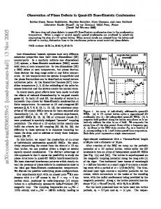
energy and magnetic field gradients will be important in determining the spatial structures of condensate, for they will compete with the energy differences between different phases. Phase diagram in finite field. When p 6= 0, the phase diagram depends on the sign of the Heisenberg interaction β. The phase diagrams for β > 0 and β < 0 are shown in Fig.2(a) and 2(b) respectively. In all cases, only the polar state P is realized as P1 and P0 are never the lowest energy states. When β > 0, (Fig.(2a)), the external field p polarizes the non-magnetic polar and cyclic states. Since Θ assumes different values in P and C, the boundary between them is first order. As p increases, both P and C gradually cross over to the ferromagnetic state. The second order phase boundary at which this occurs is p = 4β (p = 4β − γ) for the C (P) state. When β < 0, (Fig.(2b)), the only non-magnetic state is P, which will also be polarized by the external field p as in the β > 0 case. The phase boundary between the polar state and the ferromagnetic state is again a second order line, given by p = −(4|β| + γ). Of course, time-reversal symmetry is broken for all phases when p = 0. Fig.2(a) and (b) also provide a quick (qualitative) determination of the spatial spin structure of non-magnetic phases in optical traps. Since p is inversely proportional to the density n, (see eq.(4)), it generates a vertical trajectory in the phase diagram as one moves from the center of the trap to the surface of the atom cloud. Such trajectories are shown in Fig(2a) and (2b). The starting points A, B, and C indicate different kinds of spin states at the trap center. The fact that p diverges at the surface of the cloud means all non-magnetic states will develop an outer ferromagnetic layer whenever p 6= 0. The above construction does not apply to the ferromagnetic condensate as its spin structure is not affected by p. Numerical calculation including the kinetic energy is needed to determine the spatial spin configuration with fixed total magnetization. Because of the different “order parameters” Θ and hfz i, these three phases have very different spinor structures. By measuring the density in each spin component, they can be easily distinguished from each other. Finally, we note that there is a one-to-one corresponding between the structure of a spin-2 spinor Bose condensate and that of a d-wave BCS superfluids. The latter is known to be characterized by an order parameter which is a traceless 3 × 3 symmetry matrix Bij , (B = B T , TrB = 0). To see this correspondence, we note from the property of spherical harmonics that the ˆ is a homogenous polynomial of sum P (k) = k 2 ζm Y2m (k) degree 2 in k (P (k) = Bij ki kj ), and satisfies the Laplace equation ∇2k P (k) = 0. These conditions guarantee that B is a traceless symmetric matrix. We can therefore associate with each spinor a traceless symmetric matrix R ˆ ˆ Rewriting the energy in terms Bij = d4πk kˆi kˆj ζm Y2m (k). of B, one finds that eq.(4) in zero field (p = 0) reduces to the free energy of a d-wave superfluid. The exact mini-
(16) (17) (18)
One example of such spinor is s 1 iφ p2 p p T ζ = (e (1 + ), 0, 2 − 2 , 0, e−iφ (−1 + )) 2 4β 8β 4β (19) where φ is an arbitrary phase. Phase diagram in zero field. Table I summarizes the above results. When p = 0, all polar states are degenerate. By searching for the lowest energy state in Table I for given scattering lengths (hence given β and γ), we obtain the phase diagram in (γ, β)-plane as shown in the inset of Fig.1. Among the two ferromagnetic phases only the state F is realized. F′ is never the lowest energy state for all (γ, β). The three phases P, F and C are separated by the boundaries β = 0 (F-C), γ = 0 (C-P) and 4β = γ (P-F). The phases P, C, and F are characterized by the “order parameter” (|Θ| = 1, hfˆz i = 0), (Θ = 0, hfˆz i = 0), and (Θ = 0, hfˆz i = 2) respectively. Moreover, timereversal symmetry is broken for the cyclic and the ferromagnetic states but not for the polar states, where ζ ˆ ∗ are related by a phase factor, (see eq.(13)) [8]. and Aζ Since the pair (Θ, hfˆz i) undergoes discontinuous changes from one phase to another, the transition between different phases at p = 0 are all first order. It is also useful to display the phase diagram in terms of the differences in scattering lengths a0 − a4 and a2 − a4 as shown in Fig.1. The regions occupied by the three phases are : P : a0 − a4 < 0, 27 |a2 − a4 | < 51 |a0 − a4 |. F : (a2 − a4 ) > 0, 51 (a0 − a4 ) + 27 (a2 − a4 ) > 0. C : (a2 − a4 ) < 0, 51 (a0 − a4 ) − 27 (a2 − a4 ) > 0. Based on the current estimates of scattering lengths (in a.u.) by J. Burke and C. Greene [9], Spin-2 species a0 a2 a4 23 Na 34.9 ± 1.0 45.8 ± 1.1 64.5 ± 1.3 87 Rb 89.4 ± 3.0 94.5 ± 3.0 106.0 ± 4.0 +150 +100 85 Rb −445.0+100 −300 −440.0−225 −420.0−140 83 Rb 83.0 ± 3 82.0 ± 3 81.0 ± 3 we note from Fig.1 that all the three phases can be realized in the above alkali (and in fact in Rb) isotopes. The error bars in the estimates of scattering lengths, however, introduce uncertainties in the predictions of ground state structures. The case of 87 Rb is particularly unclear, for it barely resides in the polar region while the error bar covers both polar and the the cyclic states. The fact that all these realizations are close to the phase boundaries means that other physical effects such as gradient 3
mization of this problem was solved by N.D. Mermin [10]. Our zero field results are in agreement with his exact solution. Because of this correspondence, we have named the spinor phases in zero field according to the features of the d-wave solutions [10]. It is also clear from the above discussion that the structure of a spin-S spinor condensate (S = integer) corresponds to that of a singlet BCS superfluid with orbital angular momentum S. We would like to thank Eric Cornell and Carl Wieman for discussions on their experiments on 85 Rb, and to Jim Burke and Chris Greene for estimates of scattering lengths. This work was supported by NASA grant NAG8-1441 and NSF grants DMR-9808125 and DMR9708274.
F F′ C P P1 P0
1 2
�
eiφ (1 +
√1 2 √1 2
�
eiα2
p ), 0, 4β
1
2−
E 4β − 2p β −p
p2 , 0, e−iφ (−1 8β 2
p , 0, 0, 0, eiα−2 4β−γ p + 2(β−γ) , 0, eiα−1
p 1+ q
0, eiα1
ζT (1, 0, 0, 0, 0) (0, q 1, 0, 0, 0)
(0, 0, 1, 0, 0)
+
p ) 4β
p 4β−γ p ,0 2(β−γ)
p 1− q 1−
TABLE I. Possible phases in finite field
[1] J. Stenger, D.M. Stamper-Kurn, H.J. Miesner, A.P. Chikkatur, W. Ketterle, Nature, 396, 345 (1999). [2] M.R. Matthews, B.P. Anderson, P.C. Haljan, D.S. Hall, M.J. Holland, J.E Williams, C.E. Wieman, E.A. Cornell, cond-mat/9906288. [3] T.L. Ho, Phys. Rev. Lett., 81, 3355 (1998). [4] T. Ohmi and K. Machida, J. Phys. Soc. Jpn., 67, 1822 (1998). [5] T.L. Ho and S.K. Yip, cond-mat/9905339. [6] C.K. Law, H. Pu, N.P. Bigelow, Phys. Rev. Lett. 81, 5257 (1998). [7] The results were first reported in a contributed talk by Ciobanu, Yip, and Ho to the APS Centennial Meeting in March, 1999. [8] Any state with |Θ| = 1 will not have broken time-reversal ˆ ∗ |2 = 0, which implies ζ and symmetry because |ζ − ΘAζ ∗ ˆ are related by a phase factor. Using Af ˆ = f T A, ˆ it is Aζ easy to show that hf i = 0 for any state with |Θ| = 1. [9] J. Burke and C. Greene, private communication [10] N.D. Mermin, Phys. Rev. B, 9, 869 (1974)
Figure Captions Fig.1. Phase diagram in zero field. The ferromagnetic, polar, cyclic phases are denoted as F, P, and C resp. The phase boundaries P − F and P − C are straight lines with slopes −7/10 and 7/10 resp. The boundary F − C is a2 − a4 = 0. All boundaries are first order lines. The locations of various alkali isotopes on this diagram are the symbols : ⋄ =23 Na, × =87 Rb, △ =85 Rb, • =83 Rb. Inset: Zero-field phase diagram in the (γ, β) plane. Fig.2. Spinor phase diagrams in finite field for (a) β > 0 and (b) β < 0. The thick and dashed lines are first and second order phase boundaries resp. For an atom cloud with a non-magnetic state (A, B, or C) at the center, as one moves from the center to the surface, a vertical line is generated in the phase diagram, showing that the outer layer is always ferromagnetic.
4
�
�
�
2
p − 4β
γ− γ−
p2 4β−γ p2 4(β−γ)
γ
15
F a2-a4 (aB)
5
Θ ≠ 0 〈 fz〉 = 0
P
Θ = 0 〈 fz〉 = 2 83
Rb
(0,0)
-5 87
Rb
P
C
-15
23
Na 85
Rb
β
C
( 0,0 )
4β = γ
Θ = 0 〈 fz〉 = 0
F
γ
-25 -35
-25
-15
-5
a0-a4 (aB)
5
15
12
p β
8
(a)
P
B
F
4
C
A
0 -8
-4
0
4
γ β
8 6
P
F
p | β|
4
(b) γ |β| -12
2
C
0 -8
-4
0