The Reachability Problem in Constructive Geometric Constraint ...

The Reachability Problem in Constructive Geometric Constraint Solving Based Dynamic Geometry Marta R. Hidalgo Grup d’Inform` atica a l’Enginyeria Universitat Politècnica de Catalunya Barcelona, Catalonia

Robert Joan-Arinyo Grup d’Inform` atica a l’Enginyeria Universitat Politècnica de Catalunya Barcelona, Catalonia

Abstract An important issue in dynamic geometry is the reachability problem that asks whether there is a continuos path that, from a given starting geometric configuration, continuously leads to an ending configuration. In this work we report on a technique to compute a continuous evaluation path, if one exists, that solves the reachability problem for geometric constructions with one variant parameter. The technique is developed in the framework of a constructive geometric constraint-based dynamic geometry system, uses the A∗ algorithm and minimizes the variant parameter arc length. Key words: Dynamic Geometry, Constructive Geometric Constraint Solving, Reachability

1.

Introduction

Reachability is a fundamental problem in the context of many models and abstractions which describe various computational processes. Analysis of the computational traces and predictability questions for such models can be formalized as a set of different reachability problems. In general reachability can be formulated as follows: Given a computational Email addresses: [email protected] (Marta R. Hidalgo), [email protected] (Robert Joan-Arinyo).

Preprint submitted to Elsevier

4 October 2011

system with a set of allowed transformations, also called functions, decide whether a certain state of a system is reachable from a given initial state by a set of allowed transformations. Examples of applications include geographical information systems, robotics, motion planning, CAD/CAM and internet routing. In geographical navigation, reachability can be understood as helping a traveller to find feasible and safe paths to move through an unknown environment, Golledge et al. (1998). In robotics the reachability of a robot manipulator to a target is defined as its ability to move its joints and links in free space in order for its hand to reach the given target, Yang et al. (2011); Ying and Iyengar (2011). In motion planning an unmanned ground robot vehicle used in an outdoor environment over a wide variety of terrain, reachability is understood as to develop an effective path which positions and routes the friendly robotic agent in a hostile environment, Kang et al. (2010). In Internet, the routing host or gateway must supply a path of reachable routers and gateways to attempt to send datagrams to a gateway that is nearer the destination, Halabi (2000). In these applications, data are usually organized into a directed graph where the notion of ancestor-descendant relationship captures the idea of whether a node is reachable from another through a path. An emerging field where the reachability problem plays an important role is dynamic geometry, Kortenkamp (1999); Winroth (1999). Dynamic geometry is a discipline that appeared during the 80’s as a new tool in geometry. A number of software systems were designed for teaching geometry in secondary schools where the ruler and compass were replaced by computers featuring high resolution color screens for user-computer interaction. The key concept in dynamic geometry is interaction, that is, select a geometric object in the screen, move it and see immediately how the geometric construction changes. In this context, a reachability problem naturally arises and can informally be stated as follows. Let Is and Ie be two instances of a welldefined geometric construction where Is is called the starting instance and Ie the ending instance. Are there continuous transformations that, preserving the incidence relationships established in the geometric construction, brings Is to Ie ? A huge amount of literature on reachability have been published mainly in the field of abstract computational models, see for example Bournez and Potapov (2009). However there is a paucity of works concerning specific algorithms in dynamic geometry. Richter-Gebert and Kortenkamp in Richter-Gebert and Kortenkamp (2001) formalized the reachability problem in computational geometry and proved that its complexity is NP-hard in R. In Denner-Broser (2006), Denner-Broser describes a decision algorithm to solve the reachability problem in computational geometry. In a first step the algorithm computes the Voronoi diagram defined by the sites corresponding to points where the geometric construction is not feasible. Then a graph G = (V, E) is computed. V consists on a number n of copies vij , 1 ≤ j ≤ n of each Voronoi vertex vi . E is the set of pairs {(vij , vi′ j ′ )} such that {(vi , vi′ )} is an edge of the Voronoi diagram and there is a continuous transformation that starts at vij and ends at vi′ j ′ . Finally, the reachability problem is solved by checking whether the Voronoi vertices associated to the starting and ending geometric instances belong to the same connected component of G. No practical results are reported and no hints are given on whether the approach has actually been implemented.

2

1.

p1

= FREE

2.

l0

= JOIN((0,0), p1 )

3.

c1

= CIRCLE((0,0), 10)

4.

c2

= CIRCLE(p1 , 11)

5.

p2

= MEET(cl , c2 )

6.

l1

= JOIN((0,0), p2 )

7.

c3

= CIRCLE(p1 , 15)

8.

p3

= MEET(l1 , c3 )

c3

p3

c2 c1

p2

l0 (0,0)

p1

l1

Fig. 1. Left) A GSP. Right) A GSP instance.

In this work we describe a technique to decide the reachability problem in dynamic geometry. We consider ruler-and-compass geometric constructions with one variant parameter. The technique has three steps. First the set of points where the geometric construction is not feasible are computed. Then acceptable continuous transitions at these points are captured as a directed graph. Finally the reachability is decided by searching a path from the starting geometric construction to the ending construction. The search is performed by applying the A∗ algorithm. As a proof of concept, we have implemented the approach in the context of our dynamic geometry system based on constructive geometric constraint solving. Preliminary results prove that the approach is both effective and efficient from a practical point of view. 2.

Constraint-Based Dynamic Geometry

In dynamic geometry, the user is in charge of actually defining step by step the construction process that eventually will lead to the solution of the problem under study. Therefore a dynamic geometry system usefulness is basically limited by the user’s abilities. A convenient way to represent geometric constructions in dynamic geometry is Geometric Straight-Line Programs (GSP), Denner-Broser (2008); Kortenkamp (1999). A GSP consists of free points and dependent elements like a line through two points, the point where two lines intersect or the bisector of a segment. A GSPs can be seen as a sequence of construction steps such that once values have been assigned to the free points, generates an actual construction that places free and dependent elements with respect to each others. Figure 1, shows a GSP and an actual construction, In Freixas et al. (2010), Freixas et al. reported on a dynamic geometry system based on constructive geometric constraint solving. In this technology, the user defines a geometric problem by sketching some geometric elements, denoted G, taken from a given repertoire (points, lines, circles, etc) and annotates the sketch with a set of geometric relationships, called constraints, (point-point distance, point-line distance, angle between two lines and so on), denoted C, that must be fulfilled for some specific values assigned to the set of parameters, P . From now on, we shall denote a geometric problem defined by constraints as Π =< G, C, P >.

3

l1 on on p3 on

d2 d0

on

p2

d3

p0

p1

d1 on

l0 Fig. 2. Geometric problem in Figure 1 expressed as a geometric constraint solving problem.

Assuming that in the problem in Figure 1 defined at a dynamic geometry system interface, the set of geometric elements includes four points and two straight lines, G = {p0 , p1 , p2 , p3 , l0 , l1 }. Figure 2 shows an equivalent way of defining the same problem in a constraint based geometric system where d0 , d1 and d2 denote point-point distances and on denotes incidence. Many techniques have been reported in the literature that provide powerful and efficient methods for solving geometric problems defined by constraints. For a review, see Hoffmann et al., Hoffmann and Joan-Arinyo (2005). Among all the geometric constraint solving techniques, our interest here focuses on the one known as constructive. See Hoffmann et al. (2001a,b); Jerman et al. (2006); Joan-Arinyo and Soto (1997); Joan-Arinyo et al. (2001) and the references there in for an in depth discussion on this topic. Computer programs that solve geometric problems defined by constraints are called solvers. Constructive solvers, also known as decomposition-recombination planners (DR-planners), Hoffmann et al. (2001b), yield the solution to the geometric problem defined by constraints as a sequence of construction steps that places each geometric element with respect to each other in such a way that the constraints are fulfilled. Basically constructive solvers have three components: the analyzer, the index selector and the constructor. The analyzer is responsible for figuring out whether the solver is able to solve the problem up to degenerated configurations, that is, whether it can find a placement for the geometric objects such that the constraints hold. If the answer is positive, the analyzer outputs the solution as a sequence of construction steps, known as construction plan, that will place the geometric elements in the right position. Figure 3 shows a construction plan generated by a constructive solver able to solve ruler-and-compass problems, Joan-Arinyo and Soto (1997), for the problem defined in Figure 2. The meaning of each construction step is apparent. For example, origin() stands for the origin of an arbitrary framework, p1 = distD(p0 , d0 ) places point p1 at distance d1 from point p0 , c1 = circleCR(p0 , d3 ) defines the circle c1 with center p0 and radius d3 and intCC(c1 , c2 ) defines point p2 as the intersection of circles c1 and c2 . In general, the construction plan that solves a constraint problem is not unique. Construction plans generated by constructive solvers will be denoted by Γ. Solving a geometric constraint problem can be seen as solving a set of, in general, non linear equations. Therefore, each equation can have as many roots as the equation

4

1.

p0

= origin()

2.

p1

= distD(p0 , d0 )

3.

l0

= linePP(p0 , p1 )

4.

c1

c3

p3 d1 c1

c2

p2

= circleCR(p0 , d3 )

d2 d3

5.

c2


6.

p2

= intCC(c1 , c2 , s1 )

7.

l1

= linePP(p0 , p2 )

8.

c3


9.

p3

= intLC(l1 , c3 , s2 )

l0 p0

p1 d0

l1

Fig. 3. Problem in Figure 2. Left) A ruler-and-compass construction plan. Right) A construction plan instance.

degree. Obviously, each specific root will result in a different placement for the geometric elements in the problem. Selecting the desired root, known as the Root identification problem, Bouma et al. (1995), is the goal of the index selector that associates with each equation with several roots an index that unambiguously identifies the desired root. The index in the construction plan in Figure 3 is σ = {s1 , s2 } corresponding respectively to cosntruction steps 6, intersection of two circles, and 9, intersection of a line and a circle. A number of techniques have been developed to deal with the Root identification problem. See, for example, Bouma et al. (1995); Joan-Arinyo et al. (2003, 2009); van der Meiden and Bronsvoort (2005). For an in depth study of the index and the role it plays in a geometric constraint solving see Freixas et al. (2010). The specific solution to the constraint problem Π identified by an assignment of values to the index σ is called the intended solution. In what follows we consider that the solver is ruler-and-compass, that is, the degree of the equations underlying the geometric problem is at most 2. Notice that this is equivalent to say that the allowed operations in a construction plan are addition, subtraction, product, division and square root. Thus signs si in the index take values in, say, {−1, +1}. Finally, once a set of actual values have been assigned to the constraint parameters and the intended solution has been selected by assigning values to the index signs, the constructor builds an instance of a placement for the geometric objects, provided that no numerical incompatibility arises due to geometric degeneracy. This DR-planner architecture shows some nice properties. First, the nature of the computations in each step is quite different. The analyzer requires symbolic computation while the constructor only performs numerical computations. Second, determining whether the problem is solvable by the solver at hand or not is performed in the analysis step and it does not depend neither on the actual parameter values nor on the geometric computations. Next, with the proposed decoupling, when computing instances for different parameter values, only the construction step needs to be carried out. This allows to skip the analysis step, which is computationally the most expensive, as well as the index selection. Finally, given a symbolically solvable geometric constraint problem and a parameters assignment, the object can be instantiated if there are not numerical impossibilities, dividing by zero or computing the square root of a negative value. These

5

impossibilities are detected while carrying out the geometric computations and we say that the construction plan is unfeasible. 3.

Problems with One Variant Parameter

When interacting with a computer featuring a mouse as an input device, mouse cursor position as it moves around the screen is captured in discrete steps. Therefore, intermediate positions are unkown. In dynamic geometry software, it is common practice to assume that the paths of free variables between two subsequent mouse events are linear, Kortenkamp (1999). Thus, only one degree of freedom is left for the geometric element motion. In a more general framework, Denner-Broser (2006), the path is assumed to be polynomial in time t and the computation of the path itself is encoded as part of the GSP leaving just one free variable t and in this way boiling down the problem to the situation with just one free variable. In this section we present basic concepts concerning geometric constraint problems for which the value of a given constraint parameter is not fixed, that is, problems with one variant parameter. 3.1.

The Construction Plan as a Function

In general, the concept of free geometric element in dynamic geometry can be captured in constructive geometric constraint-based dynamic geometry by considering the value assigned to a given constraint as a variable value. As pointed out in Section 2, this does not have an effect on the constraint solving process and all what is needed is to reevaluate the construction plan as many times as needed. For example, the free point p1 in the GSP shown in Figure 3 can be captured by considering that the distance constraint d2 between points p1 and p2 is a variant parameter. See Figure 4. We only consider geometric problems that are wellconstrained, that is, geometric problems with a finite number of solution instances, Hoffmann and Joan-Arinyo (2005). Let Π =< G, C, P > be a well constrained geometric constraint problem such that all parameters in P have been assigned a given value except for one, say λ, which can take arbitrary values in R+ . (We only consider unsigned distances and positive angles.) We will say that the resulting problem has one variant parameter. See Figure 4. Let Γ be a construction plan that solves the constraint problem Π =< G, C, P >. Since the construction plan of a constraint problem does not depend on the specific values assigned to parameters in P , Γ is a construction plan valid for any problem derived from Π by considering one of its parameters as variant. Therefore Γ(σ, λ) defines a family of objects whose members are built as the value assigned to λ and the choices for the signs σ change. Figure 5 shows from left to right objects in the family defined by the problem in Figure 4 for distance constraint values d0 = 13, d1 = 11, d3 = 10 and values of the variant parameter λ in {4, 7, 11} and signs s1 = +1, s2 = +1. For some values of the variant parameter λ, however, it may not be possible to satisfy the set of constraints in C, that is, the construction plan Γ(σ, λ) is unfeasible for such variant parameter values. To formalize concepts related to construction plan feasibility, we need some definitions.

6

1.

p0

= origin()

2.

p1

= distD(p0 , d0 )

3.

l0

= linePP(p0 , p1 )

4.

c1

c3

p3 d1 c1

c2

p2


λ d3

5.

c2

= circleCR(p1 , λ)

6.

p2

= intCL(c1 , c2 , s1 )

7.

l1

= linePP(p0 , p2 )

8.

c3


9.

p3

= intLC(l1 , c3 , s2 )

l0 p0

p1 d0

l1

Fig. 4. Construction plan given in Figure 3 where distance d2 is considered a variant parameter, λ.

Definition 1. Let Π =< G, C, P > be a geometric constraint problem and Γ(σ, λ) a construction plan that solves Π. Assume that σ is fixed and let x = (x1 , . . . , λ, . . . , xn ) be the set of parameters in P with λ the variant parameter. If xc = (x1 , . . . , λc , . . . , xn ) is the set of parameters values where feasibility of Γ changes, we say that xc is a critical point of Γ and λc is a critical variant parameter value. To illustrate this concept, consider the construction shown in Figure 6 where a triangle is defined by giving the constraints b = distD(a, d1 ), c = distD(b, d2 ), and λ = angle(ab, ac). If we assume that d1 ≥ d2 and consider λ as the variant parameter, the construction plan shown on the left of Figure 6 is feasible for values of λ in the range [0, sin−1 (d2 /d1 )]. The bounds of this range are the critical values of λ for this construction. The situation described can be found for each basic construction in a constructive solver and the corresponding feasibility ranges can be collected in a dictionary. See Hidalgo et al. Hidalgo et al. (2011). In this context, a construction plan can be considered a function of the variant parameter and the set of signs, Γ(σ, λ). 3.2.

Continuity

The key concepts in dynamic geometry are interaction and change. If the value assigned to one constraint, the variant parameter, is interactively changed, the user expects

Fig. 5. Objects belonging to the family defined by the problem in Figure 4.

7

1.

a

= origin()

2.

b

= distD(a, d1 )

3.

c1

= circleCR(b, d2 )

4.

l

= lineP A(a, λ)

5.

c

= intCL(c, l, s)

c′

c′′

λ

c a

d1

l

d2 b

Fig. 6. Critical points for a triangle defined by two sides and the angle suported by one of them. Construction plan and actual construction.

the whole construction to follow. Moreover, whenever the variant parameter moves on continuous paths, the user expects that the geometric elements in the construction move along continuous paths as well. Since this is not always the case, we need to properly formalize this concept. In general the domain of a variant parameter is a set of disjoint intervals each bounded by critical variant parameter values. This concept is formalized in the following definitions, Freixas et al. (2010). Definition 2. Let Π =< G, C, P > be a geometric constraint problem with one variant parameter λ in P and let Γ(σ, λ) be a construction plan that solves Π. Given an index assignment, σj , we define a domain interval of the variant parameter λ as the connected set Dσi j ⊆ R+ , such that for all λ ∈ Dσi j the construction plan Γ(σj , λ) is feasible. Notice that a domain interval Dσi j bounded by the critical values λl and λu is closed in λl or in λu if Γ(σj , λl ) or Γ(σj , λu ) are instances of the construction plan Γ(σj , λ). Filled cells in Figure 7 are exemples of domain intervals. Definition 3. In the conditions of Definition 2, we define the domain of λ as the union of domain intervals for all possible index assignments in the construction plan, D(λ) = ∪i,σ Dσi (λ). Now we define a variant parameter path. (See Denner-Broser, Denner-Broser (2006), and Richter-Gerbert et al., Richter-Gebert and Kortenkamp (2001)) σ Dσ1 1

σ1 σ2

Dσ1 2 Dσ1 3

σ3

Dσ2 3

λi−1

λi

λi+1

λ

Fig. 7. Transitions at a critical parameter value in a continuous evaluation of a construction plan.

8

Definition 4. Let Γ(σ, λ) be a construction plan. With the variant parameter λ we associate a continuous path λ(t) : [0, 1] → R+ . Then we define the concept of construction plan evaluation under a movement given by a variant parameter path. Definition 5. Let Γ(σ, λ) be a construction plan with n = |σ|, the number of sings in the index. A continuous evaluation of the construction plan Γ under the movement {λ(t)} is an assignment of functions σi (t) : [0, 1] → {s}n ,

with

s ∈ {−1, +1}

such that for all t ∈ [0, 1], Γ(σi , λ(t)) is an instance of the construction plan Γ(σ, λ). If operations in a construction plan Γ(σ, λ) are continuous, a continuous evaluation of Γ makes geometric elements to move along continuous paths, as long as the variant parameter path λ(t) does not go through a critical point λc . As we said in Section 1, we build our approach on top of a ruler-and-compass solver, that is to say, we solve equations with degree at most two. Therefore, construction plans include additions, differences, products, divisions and square root operations. In this scenario, crtical points or discontinuities can appear when trying to divide by zero or computing the square root of a value equal or lower than zero. To deal with critical points in the continuous evaluation of a construction plan we introduce the concept of transition. Definition 6. Let λ(t) be a path for the continuous evaluation of the construction plan Γ(σ, λ). Let Dσi k and Dσj l be domain intervals of λ(t) such that share the critical variant parameter value λc as one bound and both domain intervals are closed in it. Let Iσck = Γ(σk , λc ) and Iσcl = Γ(σl , λc ) be two instances of the construction plan Γ. We say that the pair of instances (Iσck , Iσcl ) define a transition in the continuous evaluation of Γ for λ(t) = λc . Assuming that the domain intervals in Figure 7 are closed in the critical variant parameter λi , we can identify three transitions (Iσi 1 , Iσi 2 ), (Iσi 1 , Iσi 3 ) and (Iσi 3 , Iσi 2 ). Theorem 7. Let Γ(σ, λ) be a construction plan and λc be a critical variant parameter value. Let (Ikc , Ilc ) be a transition at λc such that they are congruent modulo rigid translations and rotations. Then the pair of instances (Ikc , Ilc ) defines a continous transition in the continous evaluation of Γ(σ, λ) at the critical value λc . Proof. Consider that once σ and λ are fixed, the instance generated by the construction plan Γ(σ, λ) is unique up to rigid translations and rotations. 2 Theorem 8. Let Γ(σ, λ) be a construction plan, and let {λi , 1 ≤ i ≤ n} be the finite set of critical points in the path {λ(t)}. Then a continuous evaluation of Γ(σ, λ) for the path λ(t) is continuous if there is at least one continuous transition at every critical variant parameter value λi . Proof. Just apply Theorem 7 to each crititcal point in the path. 2

9

σ ++

A

B

+–

C

D

–+

E

F

––

G

H

3

11.42

20.19

23

λ

Fig. 8. Domain for the driving parameter λ of the problem in Figure 4.

3.3.

The Reachability Problem

We formaly state the reachability problem we solve as follows. Let Γ(σ, λ) be a construction plan with λ the variant parameter and index σ. Let Is = Γ(λs , σs ) and Ie = Γ(λe , σe ) be respectively a starting and ending instance of Γ. Decide whether there is a continuous path λ(t) : [0, 1] → R+ of the variant parameter and assignments of index σ(t) : [0, 1] → {−1, +1}n for which there is a corresponding continuous evaluation for Γ(σ, λ) from Is to Ie . 4.

An Algorithm for the Reachability Problem

Here we describe an algorithm for deciding whether a reachability problem for a construction plan Γ(σ, λ) with just one variant parameter, as defined in Section 3.3, is or is not solvable. 4.1.

The Domain

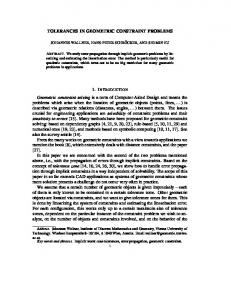
The evaluation of the construction plan depends on the actual values assigned to the parameters and on the index assignment. Parameters values fix the relative position of the geometric elements. Signs values identify the specific solution instances among the set of solution instances. In a geometric constraint problem with one variant parameter, all the parameters are fixed but one, the variant parameter. Clearly, the construction does not need to be feasible for all the values the variant parameter can take. As we have said in Section 3, in general, a domain is composed of disjoint intervals. Figure 8 illustrates the domain for the problem in Figure 4 when distance constraints values are d0 = 13, d1 = 11 and d3 = 10. Variant parameter values are represented on the X axis. Critical values where construction plan feasibility changes are 3, 11.42, 20.19 and 23. Each row in the Y axis corresponds to a set of values assigned to the signs in the index. Filled cells denote intervals of variant parameter values and index assignments for which the construction plan is feasible. To figure out the domain of the variant parameter, we apply the method developed by Van der Meiden et al., Hidalgo et al. (2011). See also van der Meiden and Bronsvoort

10

λi−1 → (λi , σ1 , Il , Iu ), (λi , σ3 , Il , Iu ) λi → (λi+2 , σ2 , Il , Iu ) λi+1 → (λi+3 , σ3 , Il , Iu ) Fig. 9. Domain represented as a bucket sort table of intervals.

(2006). We assume that the domain is given as a bucket sort with as many buckets as different critical variant parameter values are the lower bound of a domain interval. Each domain interval within a bucket stores: the upper bound of the interval domain, λu , the index σ, and the construction plan instance at each domain interval bound, Il = Γ(σ, λl ) and Iu = Γ(σ, λu ). Whenever a domain interval is open at one bound, the corresponding construction plan instance points to nil. For the domain example in Figure 7, the bucket table would be the one shown in Figure 9. 4.2.

The Routing Graph

The routing graph captures the set of possible continuos transitions in a continuous evaluation λ(t) of a given construction plan Γ(σ, λ). A node in the routing graph captures a dynamic state of the variant parameter represented by a pair (Dσi , s) with Dσi the domain interval where the variant parameter is taking values and s ∈ {+, −} defines whether the variant parameter value is actually increasing or decreasing. Arcs are directed. An arc connecting two nodes defines a continuous transition from the source node to the sink node the variant parameter value can undergo when it reaches a critical point which is a bound of a domain interval. To compute the routing graph the router explores the input domain seeking for specific interval configurations which represent continuous transitions for the variant parameter. We apply a scan-line algorithm, Foley et al. (1996). The bucket-sorted list of domain intervals is the output of computing the domain. The events that move the scan-line are the critical variant parameter values, λi . To keep track of the set of domain intervals the scan-line intersects, we define an active intervals list. For each active interval domain we store the domain interval plus a flag in the set {l, u, i} that identifies whether the scan-line intersects the domain interval at the lower bound, at the upper bound or at an interior point. When the scan-line intersects an interval domain at an interior point, the construction plan instance stored is the corresponding to the interval lower bound. Figure 10 shows the active intervals list for the domain depicted in Figure 7 as the scan-line visits the critical variant parameter values. If the domain is represented by the list of domain intervals DIL, and AIL is the active intervals list, Algorithms 1 through 3 show how we actually compute the routing graph. Figure 11 shows the routing graph yielded by this algorithm when applied to the problem depicted in Figure 4 the domain of which is given in Figure 8. Nodes for increasing λi−1 λi λi+1 λi+2 λi+3

→ → → → →

(λi , σ1 , Il , Iu , l), (λi , σ3 , Il , Iu , l) (λi , σ1 , Il , Iu , u), (λi , σ3 , Il , Iu , u) (λi+2 , σ2 , Il , Iu , l) (λi+2 , σ2 , Il , Iu , i), (λi+3 , σ3 , Il , Iu , l) (λi+2 , σ2 , Il , Iu , u), (λi+3 , σ3 , Il , Iu , i) (λi+3 , σ3 , Il , Iu , u)

Fig. 10. Active-domain intervals list for a sequence of scan lines.

11

Algorithm 1 Computing the routing graph Input: DIL, the domain intervals list Output: RG(V, E), the routing graph V=∅ E=∅ for each interval domain D in DIL do V = V ∪ {D+ , D− } E = E ∪ {(D+ , D− ), (D− , D+ )} end for AIL = ∅ Set λ to the smallest critical variant parameter value while not DIL and AIL are emptylists do Update AIL nodes Move from DIL bucket λ to de AIL the set of associated intervals Add new continuous transitions to RG Set λ to the next critical variant parameter value Remove from AIL list those intervals with ′ u′ flag end while variant parameter values are denoted X + while X − denotes decreasing variant parameter values. Notice that the graph has two disconnected components therefore, no continuous transitions between them can occur. 4.3.

Deciding Reachability

Assume that Is = Γ(σs , λs ) and Ie = Γ(σe , λe ) stand respectively for the starting and ending instances of a reachability problem stated over a geometric constraint problem with one degree of freedom, λ, that is solved by the construction plan Γ(σ, λ). It is clear that the reachability problem can be positively solved only if solution instances Is and Ie belong to the same connected components of the routing graph. Assumed that Is and Ie belong to the same connected component of the routing graph, to decide whether instance Ie can be reached from Is by a continuous evaluation of Γ(σ, λ), all what we need to do is first to identify the routing graph nodes to which Is and Ie Algorithm 2 Update AIL Nodes for each node N in ADL do if N.f lag == ’l’ then if λ < N.λl then N.f lag = ’i’ else N.f lag == ’u’ end if else if λ == N.λu then N.f lag == ’u’ end if end if end for

12

Algorithm 3 Add New Continuous Transitions for Ni , 1 ≤ i ≤ length(ADL) - 1 do for Nj , i + 1 ≤ j ≤ length(ADL) do if Ni .f lag == ’l’ and Nj .f lag == ’l’ and intervalClosed(N i .λl ) and intervalClosed(N j .λl ) and congruent(Ni .Il , Nj .Il ) then + − ), (Ni+1 , Ni+ )} E(RG) = E(RG) ∪ {(Ni− , Ni+1 else if Ni .f lag == ’u’ and Nj .f lag == ’l’ and intervalClosed(Ni .λu ) and intervalClosed(Nj .λl ) and congruent(Ni .Iu , Nj .Il ) then + − E(RG) = E(RG) ∪ {(Ni+ , Ni+1 ), (Ni+1 , Ni− )} else if Ni .f lag == ’u’ and Nj .f lag == ’u’ and intervalClosed(Ni .λu ) and intervalClosed(Nj .λu ) and congruent(Ni .Iu , Nj .Iu ) then − + E(RG) = E(RG) ∪ {(Ni+ , Ni+1 ), (Ni+1 , Ni− )} end if end if end if end for end for belong to, say X ss and X se . Then we need to search for the existence of an edge path starting in X ss and ending in X se . In general, an edge path in a routing graph that solves the reachability problem does not have to be unique. For example, Figure 12 shows two different paths that solve reachability in the geometric constraint problem given in Figure 4. Among the techniques that have been developed to select an specific path in a directed graph, if one exists, we have applied the A∗ algorithm, Russell and Norvig (2003). Our implementation, outlined in Algorithm 4, minimizes the arc lenght of the variant parameter λ. We consider some remarks concerning Algorithm 4. First, evaluations of the construction plan within a domain interval computed according either increasing or decreasing variant parameter values are indistinguishable. Thus starting and ending nodes in the routing graph should no represent states but domain intervals. We compute the collapsed routing graph from the routing graph by collapsing starting states Ds+ , Ds− into one single node Ds , and ending states, De+ , De− into one single node De . Figure 13 is the collapsed A+

B+

A-

B-

C-

C+

F-

F+

G+

G-

H+

H-

E-

E+

G-

G+

Fig. 11. Routing graph for problem in Figure 4.

13

A-

A+ C-

C+

G+ EFig. 12. Two paths that solve the reachability problem in Figure 4 if Is belongs to domain interval A and Ie belongs to interval domain G. Left) Selecting as initial state A+ . Right) Selecting as initial state A− .

graph derived from the routing graph in Figure 11. Then we feed the A∗ algorithm with the collapsed routing graph. The path-cost function used in A∗ is defined as X |λu − λl |j + ∆e λ g(λ) = ∆s λ + j

Where ∆s λ is either |λs − λu |s or |λs − λl |s depending on whether the first transition starts respectively increasing or decreasing the variant parameter. Similarly, ∆e λ is either |λe − λu |e or |λe − λl |e depending on whether the last transition ends respectively decreasing or increasing the variant parameter. Finally, |λu − λl |j is the width of the j-th domain interval traversed in the path. We define the heuristic estimate of the distance to the goal as the shortest arc of the variant parameter λ that separates the current transition instance Iσck = Γ(σk , λc ) from the ending instance Ie = Γ(σe , λe ), that is, h(λ) = |λc − λe | Let us prove that h(λ) = |λc − λe | is admissible as required by the A∗ algorithm. Theorem 9. The heuristic estimate of the distance from the current transition instance to the ending instance, h(λ) = |λc − λe |, does not overestimate the distance to the goal. Algorithm 4 Pathfinding Input: RG, the routing graph Is , starting instance Ie , ending instance Output: P, the path that leads from Is to Ie , if one exists Identify the domain interval Ds of Is Identify the domain interval De of Ie if Ds == De then P = (Ds , σs , λs , λe ) else Compute the collapsed routing graph CRG P = A∗ (CRG, Ds , λs , De , λe ) end if

14

A B+ C-

C+ G E-

B-

F-

F+

H+

HG-

E+

G+

Fig. 13. Collapsed routing graph derived from the routing graph in Figure 11 when the starting and ending domain intervals are A and G respectively.

Proof. We consider two different cases depending on the monotonicity of the continuous evaluation λ(t). First consider that λ(t) is a monotonically increasing function. Let λi , 1 ≤ i ≤ n, be the set of increasing critical variant parameter values involved in one A∗ step with λ1 the critical point that defines the current transition, as illustrated in Figure 14 Left. Let (Iσi i , Iσi i+1 ), 1 ≤ i ≤ n − 1, be the set of transitions needed to reach the ending instance, Ie . The arc length of the continuous evaluation is n−2 X

|λi+1 − λi | + |λe − λn−1 | = |λe − λ1 |

1

Thus |λe − λ1 | = |λ1 − λe | = h(λ1 , λe ). The same rational applies when λ(t) is a monotonically decreasing function. Now assume that λ(t) is not monotonic. Clearly, the continuous evaluation function λ(t) must span more than one domain interval. Consider the simplest situation depicted in Figure 14 Right where the transitions needed to reach the ending instance Ie are (Iσ11 , Iσ12 ) and (Iσ22 , Iσ23 ), After the first transition λ(t) increases and after the second one λ(t) decreases to reach λe . The λ(t) arc lenght is |λ2 − λ1 | + |λ2 − λe |. But |λ2 − λe | = |λ1 − λe | + |λ2 − λ1 |. Therefore, we have for the arc length |λe − λ1 | + 2|λ2 − λ1 | ≥ |λe − λ1 | = h(λ1 , λe ). The fact that increasing the number of intermediate transitions and the corresponding domain intervals included in the path increases the arc length of λ(t) completes the proof. 2

σ1

σ1

σ2

σ2

σ3

σ3

λ1

λ2

λe

λe λ3

λ1

λ2

Fig. 14. The heuristic estimate of the distance to the goal is admissible. Left) Monotonic continuous evaluation. Right) Non monotonic continuous evaluation.

15

A

A

C+ G

G E−

Fig. 15. Two minimum paths output by Algorithm 4 that solve the reachability problem in Figure 4. Is belongs to the domain interval A and Ie belongs to the domain interval G.

Figure 15 shows two paths with minimum variant parameter arc length computed by Algorithm 4 that solves the reachability problem for the problem in Figure 4. The starting instance Is ∈ A is defined by λs = 5 and σ = {+1, +1}, and the ending instance Ie ∈ G defined by λe = 5 and σ = {−1, −1}. The total variant parameter arc length for these paths is 16.84. 5.

Implementation and Results

Our approach to solve tracing and reachability problems has been implemented in the framework of the dynamic geometry system based on constructive geometric constraint solving described by Freixas et al. in Freixas et al. (2010). The system has two parts. One includes a user graphic interface and a constructive geometric constraint solver in charge of both defining the parametric geometric object and generating a construction plan that solves it. The other part, that we call the dynamic selector, defines the dynamic behavior of the geometric object and solves the reachability problem. To illustrate how our approach works, we show a complete case study in which the system solves a reachability problem associated to the geometric constraint problem depicted in Figure 16. The problem includes six points, pi , 1 ≤ i ≤ 5, and nine pointpoint distances whith d4 the variant parameter and distance constraint values d0 = 2, d1 = 2, d2 = 1, d3 = 1, d5 = 0.7, d6 = 0.7, d7 = 0.8, d8 = 0.89. Once the dynamic problem has been defined at the user graphic interface, the constructive geometric constraint solver computes the construction plan that solves the underlaying geometric constraint problem. For the case study at hand, the construction plan is shown in Figure 17. The system implemented has three parts: The reachability solver, the pathfinder and the simulator. The reachability solver first figures out the domain of the variant parameter as described in Sections 4.1. Next computes the routing graph using the algorithm described in Section 4.2. Figure 18 Left shows the domain of the variant parameter fior the case study. From 0.94 0.94 , I−+ ), left to right and top to bottom, arrows are the set of continuous transitions (I++ 1.44 1.44 1.86 1.86 1.86 1.86 (I++ , I−+ ), (I++ , I+− ), (I−+ , I−− ). The routing graph, which never is displayed by the system, is shown in Figure 18 Right. Although it is irrelevant, for the sake of simplicity, the implementation labels domain intervals with consecutive integers.

16

p2

d0

d5

d1

p5 d7

p4

d8

p0

p1

d4 d6 d3

d2 p3

Fig. 16. Case study: Geometric constraint problem with six points and nine point-point distances.

Once the initial and final solution instances along with the corresponding domain intervals have been defined, the pathfinder figures out the collapsed routing graph and selects a minimum path, if one exists, that solves the reachability problem applying the algorithm 4 described in Section 4.3. The resulting collapsed routing graph for the case study is shown in Figure 19 Left and the minimum path computed by the pathfinder is depicted in Figure 19 Right. Once the initial Is and ending Ie solution instances have been fixed and the collapsed graph has been computed, the simulator computes and displays at the graphic interface, a sequence of solution instances for values of the variant parameter λi+1 = λi + ∆λ with λ0 = λs such that traces the path from Is to Ie . The graphic interface is organized in three rows. See Figure 20. The top left window shows the current solution instance. The top right window displays the variant parameter domain. The window includes a vertical line placed at the current variant parameter value and a domain interval filled with light color. The current variant parameter value along with the signs of the higlighted domain interval define the current solution instance displayed on the left window. Windows in the second row provide information related to the reachability problem at hand. 1.

p0

= origin()

8.

p3

= intCC(c2 , c3 , s1 )

2.

p1

= distD(p0 , d4 )

9.

c4


3.

c0


10.

c5


4.

c1


11.

p4

= intCC(c4 , c5 , s2 )

5.

p2

= intCC(c0 , c1 , s0 )

12.

c6


6.

c2


13.

c7


7.

c3


14.

p5

= intCC(c6 , c7 , s3 )

Fig. 17. Case study. Construction plan that solves the problem.

17

σ 1

++ +–

2

3+

3-

3

–+

4

––

6

0

1+

1-

2+

2-

4+

4-

5+

5-

6+

6-

5

0.94

1.44

1.86

λ

Fig. 18. Case study. Left) Variant parameter domain. Arrows depict continuous transitions. Right) Routing graph.

The window in the bottom row provides elements for user interaction: Text fields to fix the initial and final instances, button Set to display as current instance solution the one corresponding to the selected initial instance, button Go to start the simulation, button Stop to stop the simulation and a slider to adjust the step of the variant parameter. Figure 21 shows some screen shots taken when running the system for the case study. The top left image corresponds to the initial instance and the bottom right image to the ending instance. 6.

Conclusions

In this paper we have proposed a technique to solve the reachability problem in dynamic geometry environments. In particular, geometric constructions based on constraints with one variant parameter are considered. This technique finds, if one exists, a continuous path from a given starting geometric configuration to a given ending one. The technique assumes the existence of a construction plan and is based on the analysis of the domain where the problem is solvable and the continuous transitions among domain intervals. It is divided into three steps. The first step computes the domain of the variant parameter, which captures the set of feasible, unfeasible, and critical points. The second step figures out the routing graph, which captures the set of all continuous transitions

3

3

2+

2-

5+

5-

2+

5-

6

6

Fig. 19. Case study. Left) Collapsed routing graph with initial instance within interval 6 and final instance within interval 3. Right) Minimum path that describes a solution to the reachability problem.

18

Fig. 20. Graphic interface.

between domain intervals that can be defined. Finally in the third step the A* algorithm is applied to search for a minimum path in the routing graph. The technique has been implemented on top of a dynamic geometry system based on constructive geometric constraint solving. Experimental results show that the approach is both effective and efficient from a practical point of view. References Bouma, W., Fudos, I., Hoffmann, C., Cai, J., Paige, R., June 1995. Geometric constraint solver. Computer Aided Design 27 (6), 487–501. Bournez, O., Potapov, I. (Eds.), September 23-25 2009. Reachability Problems. Vol. 5797 of LNCS, Theoretical Notes in Computer Science. Palaiseau, France.

19

Fig. 21. Case study. Screen shots of a reachability path.

20

Denner-Broser, B., 2006. On the decidability of tracing problems in dynamic geometry. In: Hong, H., Wang, D. (Eds.), LNAI 3763. Springer-Verlag, pp. 111–129. Denner-Broser, B., March 16-20 2008. An algorithm for the tracing problem using interval analysis. In: SAC’08. Fortaleza, Cear´ a, Brazil, pp. 1832–1837. Foley, J., van Dam, A., Feiner, S., Hughes, J., 1996. Computer Graphics. Principles and Practice, 2nd Edition. Addison-Wesley Pu. Co., Reading, MA. Freixas, M., Joan-Arinyo, R., Soto-Riera, A., 2010. A constraint-based dynamic geometry system. Computer-Aided Design 42, 151–161. Golledge, R., KLatzy, R., Loomis, J., Speigle, J., Tietz, J., 1998. A geographical information system for a GPS based personal guidance system. Internationa Journal Geoghraphical Information Science 12 (7), 727–749. Halabi, S., September 2000. Internet Routing Architectures, 2nd Edition. Cisco Press. Hidalgo, M., Joan-Arinyo, R., Soto, T., 2011. Computing parameter ranges in constructive geometric constraint solving: Implementation and correctness proof. Tech. Rep. LSI-11-4-R, Departament Llenguatges i Sistemes Informàtics, Universitat Politècnica de Catalunya. Hoffmann, C., Joan-Arinyo, R., 2005. A brief on constraint solving. Computer-Aided Design and Applications 2 (5), 655–663. Hoffmann, C., Lomonosov, A., Sitharam, M., 2001a. Decompostion Plans for Geometric Constraint Problems, Part II: New Algorithms. Journal of Symbolic Computation 31, 409–427. Hoffmann, C., Lomonosov, A., Sitharam, M., 2001b. Decompostion Plans for Geometric Constraint Systems, Part I: Performance Measurements for CAD. Journal of Symbolic Computation 31, 367–408. Jerman, C., Trombettoni, G., Neveu, B., Mathis, P., 2006. Decomposition of geometric constraint systems: A survey. International Journal of Computational Geometry and Applications 16, 379–414. Joan-Arinyo, R., Luz´ on, M., Soto, A., 2003. Genetic algorithms for root multiselection in constructive geometric constraint solving. Computer & Graphics 27 (1), 51–60. Joan-Arinyo, R., Luz´ on, M., Yeguas, E., 2009. Search space pruning to solve the root identification problem in geometric constraint solving,. Computer-Aided Design and Applications 6. Joan-Arinyo, R., Soto, A., 1997. A correct rule-based geometric constraint solver. Computer & Graphics 21 (5), 599–609. Joan-Arinyo, R., Soto-Riera, A., Vila-Marta, S., Vilaplana, J., April 25-28 2001. On the domain of constructive geometric constraint solving techniques. In: Duricovic, R., Czanner, S. (Eds.), Spring Conference on Computer Graphics. IEEE Computer Society, Los Alamitos, CA, Budmerice, Slovakia, pp. 49–54. Kang, M.-W., Pha, M., Hwang, D., 2010. Part i. a GIS-based simulation model for positioning & routing unmanned ground vehicles. Tech. rep., Center for Advanced Transportation and Infrastrcuture Engineering, Morgan State University. Kortenkamp, U., 1999. Foundations of dynamic geometry. Ph.D. thesis, Swiss Federal Institute of Technology Zurich. Richter-Gebert, J., Kortenkamp, U. H., 2001. Complexity issues in dynamic geometry. In: Scientific, W. (Ed.), Proceedings of the Smale Fest 2000. Foundations Computational Mathematics. pp. 1–37.

21

Russell, S., Norvig, P., 2003. Artificial Intelligence: A Modern Approach. Prentice Hall, Upper Saddle River, N.J. van der Meiden, H., Bronsvoort, W., 2005. An efficient method to determine the intended solution for a system of geometric constraints. International Journal of Computational Geometry 15 (3), 79–98. van der Meiden, H., Bronsvoort, W., 2006. A constructive approach to calculate parameter ranges for systems of geometric constraints. Computer-Aided Design 38, 275–283. Winroth, H., 1999. Dynamic projective geometry. Ph.D. thesis, Stockholms Universitet. Yang, J., Dymond, P., Jenkin, M., 2011. Exploiting hierarchical probabilistic motion planning for robot reachable workspace estimation. Informatics in Control Automation and Robotics 85, 229–241, dOI: 10.1007/978-3-642-19730-7 16. Ying, Z., Iyengar, S. S., 2011. Robot reachability problem: A nonlinear optimization approach. Journal of Intelligent & Robotic Systems 12 (1), 87–100, dOI: 10.1007/BF01258308.

22