The seasonal linear response of the Tropical Atlantic areas - Horizon ...

316

VOLUME15

JOURNAL OF PHYSICAL OCEANOGRAPHY

The Seasonal Linear Response of the Tropical Atlantic Òcean YVES DU

PENHOAT’ AND AN& MARIETREGUIER

Antenne ORSTOM, Centre Océanologique de Bretagne, 29273 Brest céda

’

(Manuscript received 9 May 1984, in final form 8 January 1985)

ABSTRACT The linear response of the tropical Atlantic ocean to climatological winds is calculated in a continuously stratified model and compared with observations. All the characteristicfeatures of the dynamic topography are reproduced at the proper locations including the series of zonally oriented ridges and troughs, the equatorial “pivot” zone and the seasonal variations of slope along the equator. Linear theory fails to explain seasonal variations of the South Equatorial Current and of the Equatorial Undercurrent, but it compares favqrably for the major zonal currents off the equator (the North Equatorial Countercurrent, the Guinea -.. Current and Undercurrent).

1. Introduction

The seasonal signal;’in thie tropical Atlantic ócean, is strong and well defined as is the annual wind cycle over the ocean. As shown in Merle (1980), heat fluxesthrough the surface cannot explain more than 10% of the heat content variatioris at the seasonal time scale. Thus we work from the assumption that, at sufficiently low frequency, the ocean response is essentially a dynamic response to wind forcing. A great number of analytic and numerical studies have been performed to understand the dynamics of the low’ frequency response to wind forcing. The first studies dealt with impulsive forcing. Both Cane and Sarachik (1981), with a shallow water model, and Philander and Pacanowski (1981), with a multilevel model, analyzed the response of the ocean to a wide range of periodic forcing. They have pointed out that its characteristics differ from the impulsive case. Busalacchi and O’Brien (1981) forced a linear reduced gravity model using observed winds to investigate the sequences of EI Niño events. The same model was run with climatological winds for the Atlantic (Busalacchi and Picaut, 1983). Gent et al. (1983) studied the semiannual cycle in the Indian ocean using a multiple baroclinic mode model. These models and the recent diagnostic study by Garzoli and Katz (1983) have been successful in demonstrating the importance of wind forcing in tropical oceans. In this work, we calculate the linear response of the tropical Atlantic to. realistic winds. The only similar study is that of Busalacchi and Picaut (1983). They used a single baroclinic mode model, with a

‘

Present affiliation: Centre ORSTOM, Dakar and Centre de Recherches Ocianographiques Dakar-Thiaroye, Dakar, Sénégal. O 1985 American Meteorological Society

realistic coastline, forced with Hastenrath and Lamb’s (1977) winds. Their model simulates the annual variations of the pycnocline depth quite well. However, it fails to reproduce the reversal of the North E q u a t o d Countercurrent (NECC) in spring and produces a ridge in mean pycnocline topography at the equator instead of a trough as is observed. The linear shallow water model is insufficient to allow quantitative comparisons with data because the ocean’s response is significantly influenced by more than one mode. Here we construct a continuously stratified linear model and calculate the vertical structure in terms of normal modes. McCreary et al. (1984) have used a similar approach to study the effect of remote annual forcing in the eastern tropical Atlantic. We use real winds (Hellerman and Rosenstein’s, 1983, wind data) to force our model. Damping is in the form of Rayleigh friction and Newtonian cooling of the same decay rate. With this simple form of dissipation the solution remains separable. We compute the dynamic height topography, which is directly comparable to historical data. Such an integrated quantity is expected to be well predicted by linear theory as indicated by nonlinear models (Cane, 1979). On the other hand, currents are not expected to be well described by linear theory and we consider how well the model results account for the observed seasonal variations of current structure. The model is described in the following section, and the model results are compared quantitatively with observed dynamic topography in Section 3. Results for the major tropical currents: the North Equatorial Countercurrent (NECC), the Guinea Current, the South Equatorial Current (SEC), the Equatorial Undercurrent (EUC) are presented in Section 4. Concluding remarks are made in Section 5.

, .

.

.

. .

’ 317

YVES D U P E N H O A T A N D A N N E M A R I E . T R E G U I E R

MARCH1985

2. The model formulation

We start with the linear equations on an equatorial @-plane.The equations are linearized about a background state taken to be a stably stratified motionless ,ocean of potential density P(z) and Brunt-Väisälä frequency ’

where po is the average density of the water column. We take the ocean bottom to be flat (H = constant) and include a mixed layer of thickness d; hence N 2 =O for O -d. This formulation is similar to Lighthill’s (1969) assumption that the wind stress acts as a body force in the mixed layer and vanishes below.

with the boundary conditions: dA,/dz = O at z = O and z = -H, where the eigenvalue C, is the phase speed associated with the mode n. The A , from a set of orthogonal functions, and have been normalized so that A,(O) = 1. The horizontal velocity, the pressure and the density are then:

: m

n=O

With H = 4000 my the barotropic mode n = O is neglected because its response is small compared to The vertical structure is solved in terms of vertical. the baroclinic ones (Moore and Philander, 1978). modes. The decomposition is obtained from the mean density profile shown in Fig. 1. This profile is b. Horizontal structure an average equatorial Atlantic profile obtained from Merle’s hydrographic data file (Merle and Delcroix, The equations of motion are nondimensionalized 1985). The vertical stkcture functionsA , are solution by the usual equatorial scaling, namely: of an eigenfunction problem and satisfy

a. Vertical structure

the velocity scale C, = (ghn)l12,where h, is the equivalent depth, the length scale Ln = (Cn/p)1/2, the time scale T, = (Cnp)-1/2.

li

40

For each n, (U,, V,, P,) satisfy the shallow water equations. Using the orthogonality properties of the eigenfunctions, we project the forcing on each mode n; letting (T”, T”)denote the wind stress,

L I !

F,

\ I

l I

i

\

FIG. 1. Background density and Bninfl-Vhdä frequency profiles: (dashed) potential density (g/cm3) and (solid) Brunt-Väisälä frequency (cph).

T”

= -,

POD,

c,=-T Y

POD,’

(4)

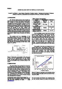
where D, = f g , ( z ) 2 d z is a wind coupling coefficient. Table 1 notes the value of D, for the different modes. Only the first three modes are significantly excited, the second one being dominant. As we are interested in seasonal variations, we make the low frequency long wave approximation:

and by scaling the shallow water equations, we find that P and U are of the same order and u = O(EU). Then, dV/dt 0(e2) and may be neglected. The horizontal structure for the mode n is then:

-

318

VOLUME15

J O U R N A L OF PH.YSICAL O C E A N O G R A P Q Y

TABLE 1. Characteristics of vertical structure. Mode number n 1 2 3

,

4

5 6 7

8

9 I

Kelvin wave speed Cß

(m 6') 2.17 1.26 0.9 1 0.64 0.49 0.39 0.33 0.30 0.21

Equivalent depth h,,

8.40

4.56 2.40 1.56 1.10 0.90 0.14

Time scale Tß (days)

Wind stress coupling coefficient O,, , (m) ,

2.78 2.12 1.80 1.5 1 1.31 1.18, 1.O8 1.03 0.98

1.65 2:16 2.54 3.03 3.48 3.88 4.23 4.45 4.66

285.4 97.2 305.4 1358. 2939.6 2006. 1093.8 425.4 516.5 .

Length

(4

16.26

scale L,,

\

,

.'

a

'

'

I

where r,, is a damping coefficient. The system (5) filters out high-frequency inertiagravity waves and short Rossby waves as well. The only allowable free solutions of Eqs. (5) are then 1) the eastward propagating equatorial Kelvin wave, 2) the westward long Rossby waves, 3) "anti-Kelvin" waves related to coastal Kelvin waves propagating energy westward due to the presence of meridional boundaries (Cane and Sarachik, 1979). The numerical procedure used to solve Eqs. (5) has been described in Cane and Patton (1984). The Kelvin wave contribution is computed by integrating along characteristics. The long-wavelength Rossby wave contribution is calculated using an 'implicit finite difference scheme on a stagered grid with a mesh size of 0.75" in longitude and 0.45" in latitude. Because this procedure has been designed around the special character of the low-frequency equatorial waves, a 10 days time step can be Ùsed (instead of hours in unfiltered models). The condition u = O is applied at the eastern boundary. Special boundary conditions are needed at the western coast because short Rossby waves generated there are no longer a solution of Eqs. (5). These waves form a boundary layer which is not explicitly computed in the model; however, their influence on the interior flow is accounted for, with the proper boundary condition

6

udy = O

(Cane and Sarachik, 1981). In the model geometry, the Gulf of Guinea and Brazilian coasts are represented by a single step. For low frequency motions,

little is gained by representing them by more than a step. The influence of such boundaries on the propagation of planetary waves is not obvious and has been described in du Penhoat et al. (1983). The basin extends from 50"W to 10"E, 18"s to 18"N; results will be presented between 10"s. and 15ON. At the northern and southern boundaries, we impose 1) = O. Analysis of results shows that closed boundaries at 18"N and 18"s do not contaminate the interior flow (an analytical demonstration is developed in Cane and Sarachik, 1979). The damping coefficient r,, is a parameter to be adjusted somewhat arbitrarily and it is commonly assumed that higher modes are more heavily damped. The dependence of the friction coefficient .on the vertical mode number may be set in various ways (Gent et al., 1983). We use McCreary's (1981) assumption that vertical damping in the basic equations has the form Y = A/N where A is a constant and N the Brunt-Väisälä frequency. We choose the constant A so that Y = 10.3 'cm2s-l over the upper 500 meters, a value in the same range as those commonly used in numerical models (Pacanowski and Philander, 1981). Then our characteristic decay time rn-' is 2 years for the first baroclinic mode, as for the standard case of Gent et al. (1983). The solution is obtained by summing over only nine vertical modes 0.73% of the wind stress project on these first nine modes. In the upper ocean (down to 600 m), they make up almost all the solution. Neglecting the perturbation stability aP'/dz compared to dj/az is a flaw of the model because, in some places unstable density profiles are generated (McCreary, 1981). These density inversions occur when there is strong vertical motion in a region with large variations in static stability. The two outstanding examples are along the equator: in the west, at the base of the mixkd layer and in the east, at the top of the thermostat. In the real ocean, these are regions of intense vertical mixing. It would be very difficult to include the physics for this process in our linear separable model.

MARCH

1985

319

Y V E S D U P E N H O A T ' A N D A N N E M A R I E TR,EGUIER

3. Results: The dynamic topography The model is spun up over three climatological years. Results are presented for the-fourth year. The monthly mean wind stress fields described in Hellerman and Rosenstein (1983) are used t6 force the model. The drag coefficient is approximated using a polynomial,, function of wind speed and air-lhinussea temperature. The data set is averaged for every month and.every 2" of longitude and latitude. In our study, the wind field is linearly inteqolated in space and time to fit the model grid. The wind field on the Atlantic ocean is characterized by northeasterly and southeasterly trade winds which converge to form the Intertropical Convergence Zone (ITCZ). The variability of the wind stress is determined 'by the seasonal displacements of the ITCZ. For instance4 is situated close to the equator in spring and winds,are,weak-atthe equator. When it reaches its northernmost position in September (about, 10'15"N) wind stress at the equator is maximum. In the western part of tge basin, the wind'%ismainly zonal and has a strong annual amplitude. In the Gulf of Guinea, the wind is more meridionally oriented'with

an eastward component at its easternmost part due to the low pressure. system on the African continent. From the density field, we compute the dynamic height anomaly relativ9 to 500 meters (see Appendix). Dynamic height plots presented below are obtained by summing over three modes. Comparing to the , sum of nine modes, 95% qf the dynamic height signal at the equator and almost 100%as we move poleward are explained by the first three modes. This can be . understood by considering that 50%of the wind stress projects on these modes, that higher modes are more heavily damped and that between O and 500 meters the gravest modes dominate the solution. Figures 2 4 show the mean; and the amplitude and phase for the annual signal obtained from historical data (Merle and Amault, 1984) and computed by the model. The two patterns are in good agreement wi$h greater'mean value and maximum amplitude in the western part of the basin. The shape of this maximum is somewhat different in, the model along the western coast because the western boundary layer has not been calculated. The model reproduces the . series of ridges and troughs of.dynamic topography which characterize the tropical Atlantic. Their posi-

/

a ............................ ........................... .................... .................... ....................

IO N

l O

10 s

40

20

10 w

O

io E

20

10 w

o

10 E

'b 10 N

O

10 5

SO

'

4b

SO

FIG.2. Dynamic height topography: annual mean (dyn cm) (a) as observed from historical data (Merle and Amault, 1984) and (b) model results.

320

VOLUME15


a

10 N

0.

1

, "

.

105 Y)

. 40

'

50

20 ,

lb'

.

-

low

*

o

loE' \

.

50

JO

20

1Q.W

O

10E

.

'

\

FIG.3. Dynamic height topography: annual amplitude (dyn cm) (a) observed and (b) model results.

tions closely correspond to those in the analyzed dynamic height field (Merle and Arnault, 1984), namely a trough at IOON, a ridge at 3"N and an equatorial trough slightly south of the equator. The southern high, located at S"S-9"S in Merle and Arnault (1 984), is poorly reproduced in Fig. 2b. As , pointed out by Busalacchi and Picaut (1983), the scarcity of wind data in the southern part of the basin is probably responsible for this discrepancy. It is worth noting that the equatorial trough in the dynamic topography is not reproduced in Busalacchi and Picaut (1983). Instead, they get an equatorial ridge. This difference could be due to our use of many modes or to a different wind data set, but it is more likely due to the difference in the numerical schemes and in boundary conditions. (A test run with their climatological wind to force our model leads to a pattern very close to our Fig. 2). A zone of minimum amplitude, located near 25OW, is associated with a rapid variation of phase separating two regions out of phase (Fig. 4).This "pivot" zone has been discussed in Merle (1980).Its position agrees with Merle and Amault (1984)'s analysis and with Busalacchi and Picaut ( 1983)'s calculation. At the equator, the mean is smaller in the east

than in observations and the gradient of mean dynamic height is 20% overestimated (Fig. 2).This may be explained noting that mean values are more sensitive than fluctuations to the average wind stress and to the damping coefficient. As this coefficient and the drag coefficient used to compute the wind stress are not precisely known and are set rather arbitrarily, we consider that the agreement between model results and data is good. Along the equator, the dynamic height gradient is directly related to the zonal wind stress T" as shown by time longitude plots (Fig. 5). In the region west of 35"W where T" is stronger, the slope is steeper than in the central region. In the easternmost part of the Gulf of Guinea, the slope reverses due to the eastward component of the winds. This reversal is more pronounced in observations (Fig. 2);this may be due to local causes such as the influence of river run off and heavy rains. At the Equator, the zonal dynamic height gradient is minimum in March-April when T x is minimum. The zonal wind stress increases first in the east and then in the west (Fig. 5). Similarly, the dynamic height gradient reaches its maximum first in the east in June and then in the west (August). The dynamic height gradient lags slightly the wind

'

MARCH1985

_

32 1

Y V E S D U P E N H O A T A N D A N N E M'ARIE T R E G U I E R

a

50

20

40

low

'

o

10 E

b

........................ ........................ ........................ ........................

IO N

O

O I 5

50

40

so

20

10 w

O

IO E

FIG.4. Phase of the annual component of the dynamic height (a) observed (in Julian days) and (b) model results (in degrees). Changes between 180" to -180" are represented by thick lines and then have no special significance (365 Julian days = 2r radians).

I

stress in the west whereas in the east, the gradient shows a stronger semiannual signal than the zonal wind stress. This probably reveals the influence of the meridional wind stress there. The computed pattern is characteristic of the periodic response of a closed basin as discussed by Cane and Sarachik (1981). It results from a complex superposition of equatorial Kelvin waves and long Rossby waves, and from their multiple reflexions and interferences. Therefore no -phase propagation can be traced back to one particular wave or wave front, as it is the case for an impulsive forcing. In the Gulf of Guinea, observations show the importance of the semiannual cycle (e.g., Picaut, 1983). The model reproduces this feature (e.g., Fig. 5b), the ratio of the semiannual and annual amplitude being greater there than in the west of the basin. Time variations of dynamic height at 4" west (Fig. 6b) exhibit a minimum slightly south of the equator in August after a rapid decrease in dynamic height corresponding to the transition between warm and cold seasons. This decrease takes place first at the equator and then moves polewards. The dynamic height pattern is qualitatively similar to the observed

sea surface temperature along 4OW (Fig. 6a; G Q U ~ ~ O U , 1983). A distinct boundary layer appears along the zonal coast of the Gulf of Guinea with a marked annual and semiannual signal. Picaut (1983) suggests that this boundary layer has the characteristics of a.single coastal Kelvin wave. This is unlikely because the graver.baroclinic mode anti Kelvin waves (Cane and Sarachik, 1979) are not trapped narrowly to the coast at these frequencies whereas the meridional scale of the coastal boundary layer is small. In the model it results from the superposition of westward propagating anti Kelvin and Rossby modes. Cane and Patton (1984) discuss the behavior of this boundary layer in some detail. They point out that it is determined by the interior flow and has less phase variations that would result from a single coastal Kelvin wave. This is confirmed in our results by the lack of net phase propagation (in Fig. 4, isophase lines are parallel to the coast). A small westward phase propagation can be detected in the results (as in observations; Picaut, 1983), but its significance is uncertain. Away from the equator, the dynamic balance changes: the equatorial Kelvin wave and the gravest

.

322

VOLUME15

J O U R N A L O F PHYSI'CAL O C E A N O G R A P H Y

a

sow

40

.

50

.

20

>low

I

'

o . . e

.

10 E

b

I

SOW

I

40

I

30

I

l

20

,

low

I

O

l

10 E

FIG.5. Time-longitude plot of (a) the zonal wind stress along the equator (averaged between 1"N and I'S) in dyn cm-*and (b) computed dynamic height along the equator (averaged between 1"N and I'S).

mode no longer matter. Higher free Rossby waves and Ekman pumping dominate the solution. Due to slow propagation of the higher Rossby modes, the dynamic height cannot adjust rapidly to the forcing on the basin scale. Consequently, the phase pattern is more complex than at the equator. In the northeast part of the basin, centered' at 25"W, 12"N there is a region of minimum mean and annual amplitude (Figs. 2 and 3). This feature, which closely corresponds to historical data, is the so called' Guinea Dome. It is a region characterized by a shallow thermocline and is more clearly evident in

northern summer when the ITCZ straddles this area (Voituriez, 198 1). It appears clearly in our calculation in July-August and reaches its dynamic height minimum of 68 dyn cm in September. The wind stress curl is upwelling favorable in the area at this time of the year, but the influence of high Rossby modes is also important and can be seen in the bending of dynamic height contours, a characteristic of Rossby mode radiation. Its southern counterpart, namely the Angola Dome, is not clearly evident in our calculation and the minimum in boreal winter is situated to the west of

MARCH 1985

Y V E S DU PENHOAT A N D ANNE M A R I E .TR,EGUIER

-

...

i

323

.

i..

FIG.6. (a) Sea surface temperature ("C) time series as observed at 4"W (Gouriou, 1983) and (b) Computed dynamic height time series at 4"W (dyn cm).

-

what observations suggest (Voituriez, 1981). The wind stress curl is small and the seasonal signal is primarily induced by Rossby waves in the model. But wind data are sparse in this area, so the estimate of the wind stress curl is somewhat imprecise.

height) because U,, P,,/Cn. Figures for the current field have been obtained by summing over nine modes. In fact, for the North Equatorial Countercurrent (NECC) and the Guinea Current, about 90% of the 9 mode response is explained by the first three.

4. The current field

a.' The North Equatorial Countercurrent

The velocity field is more dependent of higher baroclinic modes than the pressure field (or dynamic

The NECC is one of the major components of the surface current system. It is characterized by strong

u1

L

. ,

, 324

i


seasonal variations associated with wind forcing fluctuations. Its mean position is closely related to the mean position of the ITCZ. It is stronger in northern summer with maximum meridional extension. Figure 7 compares the computkd NECC with the observations (Richardson and Mc Kee, 1984) averaged between 5" and 8" North. In both time series, the current reverses in March-April and attains a maximum eastward speed around 40"W in September-October, its meridional extent then being about 5". The setup of the model NECC starts in the east and propagates westward, a feature which is also present in ship drift data (Richardson and Mc Kee, 1984). One can note the difference between model and observations at 50"W where the zonal component is westward cor'responding to the Guiana and Brasil coastal currents. These are not reproduced. because the model does not treat the western boundary layer. Away from this region, the quantitative agreement between computed and observed zonal velocities is remarkable. Furthermore, comparison between computed NECC and meridional pressure gradient- (not shown) supports the idea of geostrophic balance. , Figure 8 shows the pressure variations on the northern and southern sides of the NECC at 40"W. These variations agree with the diagnostic study by Garzoli and Katz (1983), with pressure fluctuations almost 180" out of phase between the two sides of the NECC. As pointed out earlier, the second baroclinic mode is dominant but the first mode is not negligible in either side of the current. This holds also for the zonal velocity. Figure 9 shows the relative importance of different baroclinic modes. A time longitude plot of the NECC with the second mode alone (like Fig. 7a) exhibits a similar pattern than Fig. 7a but with a much weaker amplitude and with a smaller longitudinal extension of the reversal of the flow. At the surface, the amplitude of the first and third modes are respectively '/2 and Y5 of the second mode amplitude. In summary, the pattern obtained with a single mode (namely the second one) is qualitatively comparable with data but adding modes is necessary for a quantitative comparison and to get the right amplitude of the signal as well as the right phase.

VOLUME45

a

.

so

20 w

1

b

\

b. The Guinea Current The NECC extends into the Gulf of Guinea as an eastward coastal current, the Guinea Current. In the model, it is a.boundary current with marked annual and semiannual variations. It is weak in FebruaryMarch and reaches its maximum of about 1.5 m s-' in July (Fig. IO). This closely corresponds to observations by Lemasson and Rebert (1 973). During the cold season (northern summer), its intensity is influenced by coastal effects which are not taken into account in the model. In November, it reaches a

50

45

40

35

30

LONGITUDE ,

25

20

1'5

FIG. 7. Time longitude plot of (a) computed zonal component of the NECC in m s-' (average between 5"N and 8"N) and (b) zonal velocity in the NECC in cm s-' (average between 5"N and 8"N) (Richardson and Mc Kee, 1984).

second minimum and sometimes has been observed to reverse (Lemasson and Rebert, 1973). This shows the importance of the semiannual signal in the Gulf of Guinea, well reproduced by the model. As was true for the NECC, the quantitative agreement is good. Figure 10 shows that the seasonal variations are well reproduced with the first three modes. A westward undercurrent is found from 70 m down to 400 m. It is weak (maximum 0.2 m s-l at 4"W; Fig. 11) and has a smaller amplitude than the Guinea Current. There is a time lag of about a month between the undercurrent and Guinea Current maxima. It is due to the time lag between the different modes (e.g., on Fig. 10, the first mode reaches its maximum in summer before the second mode). At depth, higher modes are not negligible (the second mode contribution is zero at 170 m) and make this

,.

m.

MARC^ ,1985

.,,.'.

,_J

,. , .

I

.

325

YVES D U PENHOAT A N D A N N E MARIE TREGUIER

,F

I M I A , Y

I

J

, J

, A

,S

, O

.I

,N , O

,

*

J I F , M , A

,

O. 4

o.

, M , J , J , A

, S , O

, N , O

b

I

.

/-\

o. o

-0.2

-0.4

- 0.6

-

0.a

I

'

I!

- 1.0

I

8' N I

I

I

(

,

- 4OoW

1

1

1

1

1

I

and (d) the sum of the first three modes: at (a) 40"W, 5"N and at (b) 4OoW, 8"N.

,

time lag more significant. The Guinëa undercurrent has been observed (Lemasson and Rebert, 1973),.but little is known about its seasonal variations. In Fig. 1 1, upward phase propagation can be seen in the vertical structure: the lag between 70 and 600 m is about 'a month. Picaut (1983) has observed a similar propagation in the temperature signal in this area. c. The South Equatorial Current and the Equatorial

Undercurrent

, ,

A

,

A

o

,,

o

FIG.9. Computed NECC annual cycle-zonal current in (m s-') averaged beween 3ON and gQN,42QWand 3O"W. Cont&ution of.(a) the first mode, (b) second mode, (c) sum of the first three modes, and (d) sum of nine modes.

In the model, high modes ( n 3 3) contribute about 50% to the South Equatorial Current (SEC). The model SEC has some resemblance to the observed one. Both have a minimum westward velocity east of 30"W in Januaiy-March (in the model, it even reverses east Of loow> and are more in March-May- The ?JXC&um speed occurs in JuneAugust. But serious discrepancies exist. The maximum

! t

i

c;

326


, -I

1

'

1

1

1

1

.

1

1

1

I

l

I

I

model of Philander and Pacanowski (198 I), westward surface currents are slowed down by vertical advection of eastward momentum 'from the Equatorial Underi.mcurrent. $.IO In a linear model, to get a permanent Equatorial Undercurrent (EUC), three conditions have to be 0.wfulfilled: the presence of a zonal pressure gradient, stratification and dissipation. In the model, the EUC 0.70is permanently prqsent at 60-70 meters depth and has a 2" half-width. Its dependance on stratification is shown by the importance of high baroclinic modes: the first three modes account for only 25% of the mean transport. However, they are dominant for the seasonal variations in the wes.tern part of the basin. -o.go The maximum speed (1.4 m s-l) occurs at 35"W in J F ' H ' A W J -J A I O N D J October whereas the maximum transport takes place FIG.10. As in Fig. 8 but for the computed seasonal cycle of the earlier (September) around 25"-3O"W (Fig. 12). It is Guinea cuqent averaged between 10"W and 4"W (m very weak (and even disappears) east of 1O"W. However, the model EUC and its variability do speed is three times the observed speed and is situ- not compare favorably with observations. The maxiated in the west instead of at 5"W (Richardson and mum speed (and the EUC transport) in the model McKee, 1984). Moreover, the semiannual' signal of decreases far more rapidly with longitude than the the SEC is present atall longitudes in observations observed one (Katz et al., 1981; Voituriez, 1983a). but is visible only west of 1O"W in model results. The discrepancies are more strikidg in the east where The meridional structure of the SEC, as described by time variations are nearly out of phasewith obser+chardson and McKee (1984), consisting of two jets vations. For instance, at 4"W in the model results, located at 2"N and 4"S, appears'in the model but is the minimum is foundin April and the maximum somewhat masked by the presence of too swift equa- in August while observations tend to show a maxitorial currents. . mum in early spring and a minimum in August Linear theory fails for the description of the surface (Voituriez, 1983a,b). We conclude that the linear equatorial currents. Shopf and Cane (1983) point out theory is not adequate for the EUC; nonlinear terms . thät at the equator, vertical transfer of momentum and a more realistic parameterization of vertical due to advection and thermodynamic processes are mixing are certainly necessary to reproduce its seasonal essential to the surface current field. In the nonlinear variations, 3.50

-

1

1

1

1

1

1

1

1

1

-

'

.

I

I

\

VOLUME15

. ._

,

..

... ..

,_ :

FIG. 11. Time versus depth plot of the zonal component u (m s-') at 4OW along the &-west coast.

MARCH1985

327

YVES D U PENHOAT A N D A N N E MARIE TREGUIER

. . ..

.

SOW

50W .

, 40

40

~

so

so

i

10 w

20

low

20

O

I .

1Ò E

10 E

FIG. 12. Time-longitude plot (a) of the model Equatorial Undercurrent transport (IO6 m3 KI)and (b) of the maximum speed (m s-I) of the model Equatorial Undercurrent. 9

5. Conclusion

at the'equator. Damping is linear and is the only arbitrary parameter in the model (There is also some We have described the response of a linear contin- freedom to choose the drag coefficient for the wind uously stratified model to the seasonal cycle of the stress). wind stress over the tropical .Atlantic Ocean. The The dynamic height topography is calculated from model equations filter out high-frequency waves and the density perturbations computed by the model. the vertical structure is calculated by summing over Occasionally, unstable profiles are generated and there nine baroclinic modes. Other modes do not contribute is no mixing mechanism in the model to homogenize significantly to the response in the upper 500 m. The the profile. However, this does not influence such an background density profile is based on observations integrated quantity as dynamic height. It turns out

c

A

328

VOLUME 15


‘that, to describe this quantity, only the first three baroclinic modes matter, the second one being dominant. We have found good quantitative agreement between historical data and model results. All the major features of dynamic height topography are present in the circulation: the ‘fpivot” -zone, the Guinea dôme, and the series of zonally oriented ridges and troughs are correctly situated. This is not the case in Busalacchi and Picaut’s (1983) calculation. Computed seasonal variations also agree with observations. Differences are small: for instance, the amplitude of the seasonal signal is too big’in the west and the mean zonal gradient along theequator is overestimated. However, as historical data- have been smoothed and have a coarser resolution, and as we did not adjust wind drag coefficient or dissipation, we believe these differ-, ences are not signifìcant. ’We then conclude that at a seasonal time scale, the dynamic height topography responds linearIy ?to wind forcing. It is a global response with the ‘dynamic height adjusting to the wind stress on the basin scale (Cane and Sarachik, 1981; Busalacchi and Picaut, 1983). . The model reproduces the. principal components of the tropical oceanic circulation, except for the western boundary currents which .are not calculated in the model. The current structure is more sensitive to higher modes than dynamic height. However, a few degrees away from the equator, the first three modes dominate- the solution and account for the seasonal variations. Good agreement is found for the North Equatorial Countercurrent (5-8 ON) and for the Guinea Current for both the mean and time variations. In the other hand, linear theory fails to explain surface .and subsurface currents in equatorial regions. The South Equatorial Current is far too strong in the west, where its maximum is found. The fixed, uniform mixed layer depth in the model is shallower than the deep mixed layer observed in the western AtIantic and this induces excessive model currents there. However, the seasonal signal agrees with observations and is in quasi-equilibrium with the zonal wind stress. There are not enough observations of the Equatorial Undercurrent to get a clear idea of its spatial and time variations. Moreover its interannual variability seems to be significant (e.g. Voituriez, 1983a; Hisard, 1973; Katz et al., 1981). Though data are sparse, we find that the model Equatorial Undercurrent does not compare well with nature. It is absent in the eastern part of the Atlantic and is found to be in equilibrium with the wind stress everywhere. This is contrary to the observations. We did not expect quantitative agreement for the Equatorial Undercurrent, but seasonal variations are not even qualitatively accounted for by the linear theory. This suggests that nonlinearities and strong vertical mixing play a significant role in Equatorial Undercurrent dynamics.

In summary, linear wind driven dynamics were shown to account for the major mean and seasonal features of dynamic topography and off-equatorial currents. Even if the basic features are qualitatively reproduced with a single baroclinic mode (the second mode), the addition of modes improves the amplitude and the phase of the signal and makes the solution directly comparable to observations.

Acknowledgments. We are indebted to Mark A. Cane for his advice and comments and for carefùlly reading an earlier version of this work. Special thanks are also due to’GillesReverdin for valuhble discussions and for his assistance in the preparation of the manuscript. This work is part of the FOCAL program and financial support was from PNEDC.

-_

.

APPENDIX

Dynamic Height Calculation

The potential density pocan be written as

‘ , In situ density is given by Miller0 and Poisson, 1981,

-

Pe

(‘42) 1 - [p(z)/k(z)l with p ( z )the hydrostatic pressure and k(z)a coefficient computed from the mean density profile. Defining a, the specific volume anomaly, to be the specific volume related to the same pressure for a temperature of 0°C and a salinity of 35% P=

a=

,

1 1 P(S, 8, P ) - P(35,OY Pl

-

. The dynamic height anomaly relative to the reference level 500 meters can be calculated by

In fact, we may write this relation more simply to show the analogy of dynamic height with other quantities as surface pressure or sea level. From (Al) we have po= pë p;: using p i < je,(A3) becomes

+

N

6 = 60 + with

c P A X , Y , 06,

n= 1

.

MARCH1985

YVES DU PENHOAT AND ANNE MARIE TREGUIER REFERENCES

Busalacchi, A. J., and J.J.O'Brien, 1981: Interannual variability of the equatorial pacific in the 1960's. J. Geophys. Res., 86, 10901-10907. ,and J.Picaut, 1983: Seasonal variability from a model of the ' tropical Atlantic Ocean. J. Phys. Oceanogr., 13, 1564-1588. Cane, M. A., 1979: The response of an equatorial ocean to simple wind stress patterns: II numerical results. J. Mar. Res.,'34, 295-432. -,and E. S. Sarachik, 1977: Forced baroclinic ocean motions: II the linear equatorial-boundedcase. J. Mar. Res., 35, 395432. -, and -, 1979: Forced baroclinic ocean motions: III the linear equatorial basin case. J. Mar. Res., 37, 366-398. -, and -, 198 I: The response of a linear baroclinic equatorial ocean to periodic forcing. J. Mar. Res., 39, 652-693. ,and R. J.Patton, 1984 A numerical model for low-frequency equatorial dynamics. J. Phys. Oceanogr, 14, 1853-1863. du Penhoat, Y., M. A. Cane and R. J. Patton, 1983: Reflexionlof low frequency equatorial waves on partial boundaries. Hydrodynamics of the Equatorial Ocean, J. C. J. Nihoul, Ed., Elsevier, 237-258. Garzoli, S. L., and E. J.Katz, 1983: The forced annual reversal of the Atlantic North Equatorial Countercurrent. J. Phys. Oceanogr., 13,2082-2090. Gent, P. R., K. O'Neill and M. A. Cane, 1983: A model of the semi annual oscillation in the equatorial Indian Ocean. J. Phys. Oceanogr., 13, 2148-2160. Gouriou, Y., 1983: Modélisation et observations des variations thermiques basse fréquence dans 1'Atlantice tropical. Internal I Rep. CNEXO-UBO, 242 pp. Hastenrath, S., and P. Iamb, 1977: Climatic Atlas of the Tropical Atlantic and Eastern Pacific Oceans. University of Wisconsin, 97 charts. Helleman, S., and M. Rosenstein, 1983: Normal monthly wind stress over the world ocean with error estimates. J. Phys. Oceanogr., 13, 1093-1 104. Hisard, Ph., 1973: Variations saisonnières i I'équateur dans le Golfe de Guinée. Cah. ORSTOM ser. Oceanogr., 11, 349358. Katz,E. J., R. L. Molinari, D. E. Cartwright, P. Hisard, H. V. Lass and A. de Mesquita, 1981: The seasonal transport of the Equatorial Undercurrent in the western Atlantic. Oceanol. Acta, 4,445-450. Lemasson, L., and J.P. Rebert, 1973: Les courants marins dans le Golfe Ivoirien. Cah. ORSTOM, Ser. Oceanogr., 11,67-95. Lighthill, M. J., 1969: Dynamic response of the Indian Ocean to

-

-f

'

-

329

the onset of the Southwest Monsoon. Phil. Trans. Roy. Soc. London, A265,45-92. McCreary, J. P., 1981: A linear stratified ocean model of the equatorial undercurrent. Phil. Trans. Roy. Soc. London, A298, 603-635. -, J. Picaut and D. W.Moore, 1984: Effects of remote annual forcing in the eastern tropical Atlantic Ocean. J. Mur. Res., 42,45-81. . McPhaden, M. J., 1981: Continuously stratified models of the steady state equatorial Ocean. J. Phys. Oceanogr., 11, 337354. Merle, J.; 1980: Seasonal heat budget in the Equatorial Atlantic . Ocean. J. Phys. Oceanogr., 10,464-469. -, and S . Amault, 1984 Seasonal variability of the surface dynamic topography in the Tropical Atlantic Ocean. J. Mar. Res. [in press.] -,and T. Delcroix, 1985: Seasonal variability of the thermocline topography in the tropical Atlantic ocean. Submitted to J. Phys. 'Oceanogr. Millero, F. J., and A. Poisson, 1981: International one atmosphere equation of state of sea water. Deep Sea Res., 28,625629. Moore, D. W., and S. G. H. Philander, 1978: Modeling of the tropical oceanic circulation. The Sea, Vol. 6, E. D. Goldenber&I. N. Cave, J. J. O'Brien and J. H. Steek, Eds., WileyInterscience, 3 19-361. Pacanowski, R. C., and S. G. H. Philander, 1981: Parametrization of vertical mixing in numerical models of tropical oceans. J. Phys. Oceanogr., 11, 1443-1451. Philander, S. G. H., and R. C. Pacanowski, 1981: Response of equatorial oceans to periodic forcing. J. Geophys. Res., 86, 1093- 19 16. Picaut, J., 1983: Propagation of the seasonal upwelling in the Eastern Equatorial Atlantic. J. Phys. Oceanogr., 13, 18-37. Richardson, P. L., and T. K. Mc Kee, 1984: Average Seasonal Variation of the Atlantic North Equatorial Countercurrent from ship drift data. J. Phys. Oceanogr., 14, 1226-1238. Schopf, P. S., and M. A. Cane, 1983: On equatorial dynamics, mixed layer physics and sea surface temperature. J. Phys. Oceanogr., 13, 917-935. Voituriez, B., 1981: Les sous courants équatoriaux Nord et Sud et la formation des dômes thermiques tropicaux. Oceanol. Acta., 4,497-506. -, 1983a: Les variations saisonnièkes des courants équatoriaux 2 4"W et I'upwelling équatorial du Golfe de Guinée. 1) Le sous courant équatorial. Oceanogr. Trop., 18, 163-183. -, 1983b: Les variations saisonnières des courants équatoriaux 5 4"W et I'upwelling équatorial du Golfe de Guinée. 2) Le courant équatorial sud. Oceanogr. Trop., 18, 185-199.

j I

-

Reprinted from JOURNALOF PHYSICAL OCEANOGRAPHY, VOI. IS, NO. 3. Amcrican Mcicorological Society Printed in U. S. A.

aic ch 1985

The Seasonal Linear Response of thi Tropical Atlantic Ocean I

YVES DU m N H O A T AND ANNE MARIETREGUIER

\

!

,

Fonds Documentaire ORSTOM

.

-Y

Fonds Documentaire ORSTOM