I would like to thank Jim Morgan who has had limitless enthusiasm for this project, ...... [115] P. W. Anderson, D. J. Thouless, E. Abrahams, and D. S. Fisher, Phys.
THE SIMULATION OF THE ELECTRONIC TRANSPORT PROPERTIES OF NANOSCALE DEVICES
By Keith Patrick McKenna
SUBMITTED IN ACCORDANCE WITH THE REQUIREMENTS FOR THE DEGREE OF DOCTOR OF PHILOSOPHY
UNIVERSITY OF LEEDS DEPARTMENT OF PHYSICS AND ASTRONOMY LEEDS AUGUST 2005
The candidate confirms that the work submitted is his own and that appropriate credit has been given where reference has been made to the work of others. This copy has been supplied on the understanding that it is copyright material and that no quotation from the thesis may be published without proper acknowledgement.
i
List of Tables 1.1
Slater and Koster’s table of the angular dependance of interatomic hopping matrix elements as a function of the direction cosines, l, m, and n. . . . . . . . . . . . . . . . . . . . . . . . . . . . . . . . . . . .
3.1
26
Equivalent quantities used to characterise the D.C. transport properties of a system. . . . . . . . . . . . . . . . . . . . . . . . . . . . . . .
75
3.2
Conversion from Rydberg units to SI for some important quantities. .
82
5.1
Time line of research in GMR. . . . . . . . . . . . . . . . . . . . . . . 115
5.2
Spin-relaxation times in copper and cobalt calculated using the EOM method. . . . . . . . . . . . . . . . . . . . . . . . . . . . . . . . . . . 138
ii
List of Figures 1.1
Illustration of the muffin-tin potential used in APW calculations. . .
16
1.2
Energy bands for copper calculated using Slater’s APW method. . . .
17
1.3
The spin-dependent electronic structure for a ferromagnetic transition metal. . . . . . . . . . . . . . . . . . . . . . . . . . . . . . . . . . . .
22
1.4
Illustration of typical matrix elements in tight-binding. . . . . . . . .
27
1.5
A comparison between an APW calculation and a simple TB parameterisation for Ni. . . . . . . . . . . . . . . . . . . . . . . . . . . . . .
30
1.6
Tight-binding parameterisation for Ge. . . . . . . . . . . . . . . . . .
32
2.1
Interface resistance between two free-electron-like materials calculated using the Landauer formula. . . . . . . . . . . . . . . . . . . . . . . .
43
2.2
Spin-dependent transmission probabilities for Cu/Co (001). . . . . . .
45
2.3
The layer-by-layer recursive Green’s function method for a multilayer system. . . . . . . . . . . . . . . . . . . . . . . . . . . . . . . . . . . .
3.1
Current flowing through a nanoscale structure between leads at L and R. . . . . . . . . . . . . . . . . . . . . . . . . . . . . . . . . . . . . .
3.2
70
The norm of the wavefunction and the current density as a function of time. . . . . . . . . . . . . . . . . . . . . . . . . . . . . . . . . . . . .
3.5
69
Reflection coefficient of a semi-infinite 1D chain of s-orbitals terminated by a site with an imaginary energy component, -iη. . . . . . . .
3.4
65
A semi-infinite one dimensional chain of s-orbitals terminated by a site with an imaginary energy component, -iη. . . . . . . . . . . . . . . .
3.3
55
72
The norm of the wavefunction averaged within the planes perpendicular to the direction of current flow. . . . . . . . . . . . . . . . . . . .
74
3.6
Spectral analysis of the wavefunction integrated using the LF method indicating the unstable additional eigenstates. . . . . . . . . . . . . .
79
4.1
Important electronic properties of the simple cubic s-orbital model. .
86
4.2
The resisitivity per spin of a homogeneously disordered simple cubic system calculated using the EOM method and compared with the Boltzmann equation. . . . . . . . . . . . . . . . . . . . . . . . . . . .
4.3
The temperature dependence of the resistivity calculated using the EOM method. . . . . . . . . . . . . . . . . . . . . . . . . . . . . . . .
4.4
98
Two interfaces which transmit well for a narrow range of electron trajectories indicating subtle interface proximity effects. . . . . . . . . .
4.9
97
The steady state norm of the wavefunction and current density in the CIP geometry . . . . . . . . . . . . . . . . . . . . . . . . . . . . . . .
4.8
94
The model system used for the CIP geometry. The right contact is separated from the structure to make the layers visible. . . . . . . . .
4.7
93
A trilayer with the same disorder ratio, W/V = 2, throughout but with different hopping matrix elements in each layer. . . . . . . . . . . . .
4.6
90
The steady state chemical potential profile in a trilayer with constant hopping matrix throughout, V = 1eV, but with varying disorder. . . .
4.5
88
99
The two configurations used to define the interface resistance. . . . . 100
4.10 The time-averaged norm of the wavefunction averaged over the planes for the two configurations. . . . . . . . . . . . . . . . . . . . . . . . . 101 4.11 The calculated interface resistance as a function of the separation between B layers, LA . . . . . . . . . . . . . . . . . . . . . . . . . . . . . 102 4.12 The effect of structural disorder on the interface resistance. (a) The resistances of configurations I and II. (b) The calculated interface resistance compared with a simple Boltzmann calculation. . . . . . . . 104 5.1
Comparison of the DOS of the parameterised TB model with a modern ASW calculation. . . . . . . . . . . . . . . . . . . . . . . . . . . . . . 109
5.2
Illustration of the origin of the CPP GMR effect. . . . . . . . . . . . 114
5.3
The simple model systems used to investigate the role of the meanfree-path. . . . . . . . . . . . . . . . . . . . . . . . . . . . . . . . . . 118
5.4
Effect of Anderson disorder on the resistance of each spin-channel. . . 119 iii
5.5
Effect of disorder on CPP GMR for interleaved and separated configurations. . . . . . . . . . . . . . . . . . . . . . . . . . . . . . . . . . . 121
5.6
Dependence of the non-local part of the interface resistance for spin up in the interleaved configuration (parallel magnetic alignment). . . . . 122
5.7
The DOS for of a Co/Cu multilayer calculated using the EOM method. 124
5.8
A Cu/Co multilayer with fcc crystal structure. 100 direction is parallel to the z-axis. . . . . . . . . . . . . . . . . . . . . . . . . . . . . . . . 126
5.9
Norm of the wavefunction in steady-state averaged within the planes perpendicular to current flow for the Cu12 Co4 Cu3 Co4 Cu12 structure. . 127
5.10 The variation of the spin-orbit parameter, ξ, across the periodic table. 133 5.11 Effect of integration time on the shape of the filter function. . . . . . 135 5.12 Spectral weight of the filtered wavefunction showing the eigenstates at the Fermi energy. . . . . . . . . . . . . . . . . . . . . . . . . . . . . . 137 5.13 Spin-relaxation in copper and cobalt. There is no disorder present and box boundary conditions are used. . . . . . . . . . . . . . . . . . . . . 138 5.14 Spin-relaxation in copper with periodic boundary conditions applied. As the strength of disorder in increased the spin-flip rate increases. . 139 5.15 Injection of a spin-polarised current into Cu with strong spin-orbit coupling. . . . . . . . . . . . . . . . . . . . . . . . . . . . . . . . . . . 141 5.16 The effect of the spin-orbit interaction on the resistivity of a highly resistive system. . . . . . . . . . . . . . . . . . . . . . . . . . . . . . . 143 A.1 The self-consistent electrochemical potential in a one-dimensional wire. 153 B.1 The calculation of the DOS using an EOM method. . . . . . . . . . . 157
iv
v
Acknowledgements I would like to thank Jim Morgan who has had limitless enthusiasm for this project, and has given me endless support and encouragement. Bryan Hickey for the many stimulating discussions we have had, and for the help he has given me. Lisa Michez who worked on the project preceding this one and has passed a great deal of knowledge on to me. I thank Geoff Davies for kindly allowing me to use the Maxima supercomputer, and Alan Real for his detailed knowledge of OpenMP. Also Aidan Hindmarch for answering numerous experimental questions for me, discussing physics frequently in the Fenton, and for help with LATEX. I would also like to thank anyone I haven’t already mentioned from the Physics department at Leeds as I have had useful and interesting conversations with many of you. I gratefully acknowledge the funding of this project by a University of Leeds Research Scholarship. On a more personal note, I would like thank my family for their support over the years. Cat, for being so kind and understanding while I have been writing this thesis. Also everyone in the condensed matter group, past and present, for the many good times I have had during my time there.
vi
Abstract A quantum-mechanical equation of motion simulation for electronic transport has been developed. A tight-binding basis is used, which has the advantages that complex electronic structures can be described and systems with arbitrary geometry can be considered. It is used to investigate fundamental issues for transport in complex and inhomogeneous nanoscale systems. The technique is applied to a number of simple systems to verify the validity of the approach and to investigate its potential scope. The method is also applied to a number of important problems in the field of spintronics. Current-perpendicular-tothe-plane giant magnetoresistance (CPP GMR) in thin film magnetic multilayers is simulated, and non-local interfaces resistances associated with mean-free-path effects are considered. Conduction electron spin-relaxation is also simulated by incorporating the spin-orbit interaction into the method. Spin-relaxation times for the technologically important materials copper and cobalt are calculated, and its effect on transport is simulated. A significant mean-free-path effect is observed for a simple model of CPP GMR. The non-local part of the interface resistance is found to depend upon the ordering of layers in a multilayer, and upon the size of the mean-free-path. However the GMR is barely modified by these effects, and an interpretation is given which explains recent theoretical and experimental results on similar systems. A GMR of 67% is calculated for a realistic device structure, Co4 Cu3 Co4 , and the effect is found to be dominated by spin-dependent interface resistances. The direct simulation of spin-relaxation by the incorporation of the spin-orbit interaction is the first such calculation of its kind. Spin relaxation times of 25ps and 0.4ps, for Cu and Co respectively have been calculated - assuming realistic resistivities. These times are in good agreement with recent optical and transport measurements.
vii
Table of Contents List of Tables
i
List of Figures
ii
Acknowledgements
v
Abstract
vi
Table of Contents
vii
Publications
x
Abbreviations
xi
Introduction
1
1 Electronic structure 1.1 Introduction . . . . . . . . . . . . . . . . . 1.2 Band structure methods . . . . . . . . . . 1.2.1 Augmented plane waves . . . . . . 1.2.2 Pseudo-potentials . . . . . . . . . . 1.2.3 Korringa-Kohn-Rostoker technique 1.2.4 Spin dependent electronic structure 1.3 Tight-binding . . . . . . . . . . . . . . . . 1.3.1 Formalism . . . . . . . . . . . . . . 1.3.2 Justification of tight-binding . . . . 1.3.3 Band structure calculations . . . . 1.4 Summary . . . . . . . . . . . . . . . . . . 2 Electronic transport 2.1 Introduction . . . . . . . . . . . . . . 2.2 General concepts . . . . . . . . . . . 2.2.1 The electrochemical potential 2.2.2 Quantum-mechanical effects . 2.2.3 Interface resistance . . . . . .
. . . . .
. . . . .
. . . . .
. . . . . . . . . . .
. . . . .
. . . . . . . . . . .
. . . . .
. . . . . . . . . . .
. . . . .
. . . . . . . . . . .
. . . . .
. . . . . . . . . . .
. . . . .
. . . . . . . . . . .
. . . . .
. . . . . . . . . . .
. . . . .
. . . . . . . . . . .
. . . . .
. . . . . . . . . . .
. . . . .
. . . . . . . . . . .
. . . . .
. . . . . . . . . . .
. . . . .
. . . . . . . . . . .
. . . . .
. . . . . . . . . . .
. . . . .
. . . . . . . . . . .
. . . . .
. . . . . . . . . . .
13 13 16 16 18 19 20 22 22 27 28 33
. . . . .
34 34 36 36 38 40
viii
2.3
2.4
2.2.4 Spin-dependent transport . . . . . . . . . . . . . Transport formalisms . . . . . . . . . . . . . . . . . . . . 2.3.1 Boltzmann equations . . . . . . . . . . . . . . . . 2.3.2 The Kubo formula . . . . . . . . . . . . . . . . . 2.3.3 The Landauer-B¨ uttiker formalism . . . . . . . . . 2.3.4 Layer-by-layer recursive Green’s function method 2.3.5 Equation of motion methods . . . . . . . . . . . . Summary . . . . . . . . . . . . . . . . . . . . . . . . . .
3 Quantum simulation of electronic transport 3.1 Introduction . . . . . . . . . . . . . . . . . . 3.2 Equation of motion simulation . . . . . . . . 3.2.1 Basis of the method . . . . . . . . . 3.2.2 Boundary conditions . . . . . . . . . 3.2.3 Definition of the conductance . . . . 3.3 Numerical methods . . . . . . . . . . . . . . 3.3.1 Forward difference method . . . . . . 3.3.2 Leapfrog method . . . . . . . . . . . 3.3.3 Runge-Kutta . . . . . . . . . . . . . 3.3.4 Atomic-units . . . . . . . . . . . . . 3.4 Summary . . . . . . . . . . . . . . . . . . .
. . . . . . . . . . .
. . . . . . . . . . .
. . . . . . . . . . .
. . . . . . . . . . .
. . . . . . . . . . .
. . . . . . . . . . .
. . . . . . . . . . .
. . . . . . . .
. . . . . . . .
. . . . . . . .
. . . . . . . .
. . . . . . . .
. . . . . . . .
. . . . . . . .
42 44 45 48 51 53 56 58
. . . . . . . . . . .
. . . . . . . . . . .
. . . . . . . . . . .
. . . . . . . . . . .
. . . . . . . . . . .
. . . . . . . . . . .
. . . . . . . . . . .
59 59 60 60 64 70 75 76 77 79 81 81
. . . . . . . . . .
83 83 86 86 88 90 91 92 99 103 104
. . . . . . . . .
106 106 108 108 110 111 112 112 117 127
4 Development of simulation method 4.1 Introduction . . . . . . . . . . . . . . . . . . . . . . . . . . 4.2 Homogeneous systems . . . . . . . . . . . . . . . . . . . . 4.2.1 Comparison with the Boltzmann equation . . . . . 4.2.2 Finite temperature calculations . . . . . . . . . . . 4.3 Inhomogeneous systems . . . . . . . . . . . . . . . . . . . 4.3.1 Variation of disorder . . . . . . . . . . . . . . . . . 4.3.2 Variation of electronic structure . . . . . . . . . . . 4.3.3 Interface resistance of multilayers . . . . . . . . . . 4.3.4 Effect of structural disorder on interface resistance . 4.4 Summary . . . . . . . . . . . . . . . . . . . . . . . . . . . 5 Simulations of spintronic systems 5.1 Introduction . . . . . . . . . . . . . . . . . . . . . . 5.2 Magnetism . . . . . . . . . . . . . . . . . . . . . . . 5.2.1 Electronic structures . . . . . . . . . . . . . 5.2.2 Temperature dependence of ferromagnetism 5.2.3 Finite size effects . . . . . . . . . . . . . . . 5.3 CPP Giant magnetoresistance . . . . . . . . . . . . 5.3.1 Theory and background . . . . . . . . . . . 5.3.2 CPP GMR calculations . . . . . . . . . . . . 5.3.3 Summary . . . . . . . . . . . . . . . . . . .
. . . . . . . . .
. . . . . . . . .
. . . . . . . . .
. . . . . . . . .
. . . . . . . . . .
. . . . . . . . .
. . . . . . . . . .
. . . . . . . . .
. . . . . . . . . .
. . . . . . . . .
. . . . . . . . . .
. . . . . . . . .
. . . . . . . . . .
. . . . . . . . .
ix 5.4
5.5
Conduction electron spin relaxation . . . 5.4.1 Theory and background . . . . . 5.4.2 Spin-relaxation time calculations 5.4.3 Transport effects . . . . . . . . . 5.4.4 Weak localisation . . . . . . . . . Summary . . . . . . . . . . . . . . . . .
. . . . . .
. . . . . .
. . . . . .
. . . . . .
. . . . . .
. . . . . .
. . . . . .
. . . . . .
. . . . . .
. . . . . .
. . . . . .
. . . . . .
. . . . . .
. . . . . .
. . . . . .
. . . . . .
128 129 133 140 141 144
6 Conclusions 145 6.1 Conclusions . . . . . . . . . . . . . . . . . . . . . . . . . . . . . . . . 146 6.2 Future work . . . . . . . . . . . . . . . . . . . . . . . . . . . . . . . . 148 A Self-consistent electrochemical potentials
151
B Equation of motion method for the density of states
154
References
158
x
Publications ‘Quantum transport simulation based on an equation of motion method: an application to current-perpendicular-to-the-plane giant magnetoresistance’ K. P. McKenna , L. A. Michez, G. J. Morgan and B. J. Hickey. Phys. Rev. B 72, 054418 (2005)
xi
Abbreviations AF:
Anti-Ferromagnet
AMR:
Anisotropic Magnetoresistance
APW:
Augmented Plane Wave
BZ:
Brillouin Zone
CIP:
Current in the Plane
CGA
Conjugate Gradient Approximation
CPP:
Current Perpendicular to the Plane
D.C.:
Direct Current
DF:
Distribution Function
DFT:
Density Functional Theory
DOS:
Density of States
EC:
Electrochemical
EOM:
Equation of Motion
FET:
Field Effect Transistor
GMR:
Giant Magnetoresistance
KKR:
Korringa-Kohn-Rostoker
LCAO:
Linear Combination of Atomic Orbitals
LDA
Local Density Approximation
LDOS:
Local Density of States
LRGF:
Layer-by-layer Recursive Green’s Function
MBE:
Molecular Beam Epitaxy
MRAM:
Magnetic Random Access Memory
MTO:
Muffin-Tin Orbital
OPW:
Orthogonalised Plane Wave
QD:
Quantum Dot
xii RK:
Runge-K¨ utta
RKKY:
Ruderman-Kittel-Kasuya-Yosida
TB:
Tight-Binding
TDSE:
Time Dependent Schr¨odinger Equation
TMR:
Tunneling Magnetoresistance
SCHF:
Self-Consistent Hartree-Fock
SGF:
Surface Green’s Function
WDF:
Wigner Distrubution Function
1
Introduction This thesis is concerned with simulating the electronic transport properties of very small nanoscale structures. The work is focussed primarily on spin-dependent transport in thin film magnetic multilayers, however many of the ideas presented apply more generally. Such systems represent an important challenge as they are highly inhomogeneous and the electronic structure can be very complex - if magnetic transition metals are present for instance. The simulation of transport in these systems is technological relevant as they have numerous applications in the computer industry, magnetic random access memory [1] (MRAM) and hard disk read heads for example. Such devices are becoming increasingly small as Moore’s law continues to be obeyed, and quantum effects become more and more important. Given the title of this thesis it is important at the outset to clarify which types of device one is referring to with the adjective ‘nanoscale’. The prefix ‘nano’ derives from the ancient Greek word ν α ˆ νoς meaning dwarf, and was adopted as the syst`eme international d’unit´es (SI) standard notation for 10−9 in 1960. In recent years it has had prolific use in a range of scientific disciplines; nanorobotics, nanoengineering, nanoelectronics and nanofabrication are just a few examples. In many cases it is not at all clear to what the prefix pertains. The Oxford English Dictionary [2] defines this new usage of the word as pertaining to length scales between 1-100nm, although it is certainly not the case that this convention is applied universally. In the context of this thesis nanoscale will be taken to mean that at least one, or possibly every one, of the dimensions of a system has extension less than or of the order of 100nm.
2 In solid state structures typical interatomic separations are of the order of 0.5nm, therefore the nanoscale systems to be considered may extend less than 200 atoms in some directions. In many cases of interest there is only one dimension that has this length-scale while the other two are essentially macroscopic - this is the case for thin film multilayers which are discussed shortly. An important point to note is that nanoscale systems can contain a large number of atoms; a system with an extension of around 50nm in all three dimensions contains of the order 106 atoms. Even for very small systems it is rarely possible to attempt a complete solution of the problem using methods such as density functional theory (DFT) or self-consistent HartreeFock (SCHF) [3] for example. As is the case for larger systems many approximations must be made to make further progress. The simulation techniques developed in this thesis will need to apply to systems containing anywhere between several hundred to up to and over one million atoms. Nanoscale systems There are many interesting devices that fall into this nanoscale category, ranging in size and complexity from individual molecules [4] (several nm) to complicated semiconductor heterostructures (∼ 100nm). There are now so many interesting nanoscale systems that it would be impossible to give a short review and do justice to all of them – accepting this and understanding that any omissions do not imply those systems are uninteresting – a brief discussion of some important types of system will follow, with particular emphasis on their electronic transport properties. Quantum dots A quantum dot (QD), to put it simply, is a very small region where electrons (or holes) are confined. They can be fabricated in a number of ways and typical dimensions do not exceed 500nm, but can be as small as tens of nanometres. Leads may be attached to a QD to measure its conductance and the contacts must be much smaller
3 than the dot itself. QDs have very interesting transport properties which are highly sensitive to their environment. Many of these effects are caused by electrons entering the QD from the lead significantly perturbing to the dot itself - through the Coulomb interaction for example [5]. One common method to fabricate a QD makes use of a two dimensional electron gas (2DEG) [6]. A 2DEG can be formed at the interface between two semiconductors that have different band gaps, AlGaAs/GaAs for example. If the Al doping is sufficient (∼30% of Ga replaced by Al) the Fermi energy can be pushed above the bottom of the conduction band inside an essentially two-dimensional region at the interface. At low temperatures the electrons in this region have a very high mobility parallel to the interface. If metallic films are grown in certain regions onto this structure and a large negative voltage applied electrons can be excluded from these regions. A QD can be defined on a 2DEG with two point contacts supplying the current. It can be defined in any shape and any size, the only limitation being difficulty in fabrication. An additional metallic contact can be placed inside the dot to modify its electrostatic properties by the application of a voltage (this voltage is called the gate voltage in analogy with traditional transistor devices). QD systems have been studied intensively to investigate electron-electron interactions [7], and also the effects of quantum chaos [8]. Carbon Nanotubes Carbon nanotubes were discovered relatively recently (1991) by Sumio Iijima [9] in experiments originally designed to study the synthesis of fullerenes. They consist of hexagonally arranged two dimensional planes of carbon (graphite sheets) that are rolled up into closed cylinders. The lengths of these tubes can be of the order of microns with diameters that can be smaller than 1nm. Nanotubes are theoretically expected to have remarkable mechanical, electronic, and optical properties and this has stimulated a great deal of research [10].
4 The electronic properties are determined by the spatial arrangement of the carbon atoms. The nanotubes can form a cylinder in different ways identified by their chirality. The periodicity around the circumference of the nanotube sets up standing waves and thereby defines various one-dimensional conduction modes. It has been predicted that nanotubes with certain chirality are metallic while others are semiconducting [11]. This raises the interesting possibility of multiwall nanotubes consisting of a metallic nanotube inside a semiconducting one. The metallic nanotube could dope the semiconductor and produce a highly conducting 1D wire or nanowire [12]. Nanowires would find many useful applications in the computing industry, connecting nanoscale memory and processor components for example with low power consumption. Thin film multilayer structures Thin film multilayers consist of consecutive films of material, which can range in thickness from partial monolayers to hundreds of monolayers, grown in a sandwich structure. There structures can contain a very wide range of materials, and many examples have technological applications. Various fabrication techniques are used such as sputtering and molecular beam epitaxy (MBE) - each with their own subtle advantages. The thickness of these systems in the growth direction (perpendicular to the layers) is very small - usually much less than 100nm. The materials that can be used in these structures include almost all solid state materials, and in most cases the interesting effects that occur arise from the complicated electronic and magnetic properties of the materials used. The field of spintronics is concerned with the transport of spin as an additional degree of freedom aside from the charge of the electron. This idea is being investigated intensively in magnetic multilayer structures. Giant magnetoresistance (GMR) [13] is an effect that occurs in multilayer structures that consist of a series of ferromagnetic (FM) layers separated by paramagnetic (PM) spacer layers. A typical structure may contain 20 [PM/FM] repeats. If the
5 thickness of the PM spacer layers is chosen correctly, adjacent FM layers can be magnetically coupled anti-parallel to each other by a Ruderman-Kittel-Kasuya-Yosida (RKKY) type of interaction [14, 15, 16]. On application of a small external magnetic field the FM layers can be aligned parallel, and a large change in the resistance of the multilayer is observed (of the order 100%). This GMR effect can be measured with current flowing parallel to the planes of the layers (CIP), or perpendicular to the planes (CPP), but the effect is generally larger in the later geometry. So called spin valve devices [17] may also be fabricated; in which just two FM layers are separated by a single PM layer. In order that the magnetic configuration of the FM layers can be switched by application an external magnetic field one of the FM layers is pinned by an exchange biased anti-ferromagnetic (AF) layer. The magnetisation of the unpinned FM layer is free to follow any externally applied field no matter how small it is; a much larger field is required to rotate the magnetisation of the pinned layer. The advantage of a spin valve is that a very small external magnetic field will cause the magnetisations to align parallel as the FM layers are not directly magnetically coupled - it is this sensitivity that led to its application in hard-disk read heads. A related phenomena to GMR is the tunneling magnetoresistance (TMR) effect [18]; it is observed in structures where two FM layers are separated by a thin insulating layer, with current flowing perpendicular to the planes. The magnitude of the effect in these systems can be much larger than is observed for GMR, up to 1000% in Fe/MgO/Fe for example [19]. The very different decay lengths for different electronic states in the insulator is the origin of this much larger effect. As the effect is very sensitive to the nature of electronic states, TMR can provide a means to probe the electronic structure of magnetic materials [20]. Many of the nanoscale systems that have been discussed here have potential device applications for information storage and processing. In fact many of these devices
6 have already been developed for industry. Important future applications of nanoscale solid state systems are likely to be in the emerging field of quantum computation. The theory of this new subject is already quite advanced [21], but the practical realisation of a qubit represents a very difficult problem. Many of the most promising possibilities being explored involve spintronic solid state devices [22]. It is certain that these systems will continue to be an active area of research for the considerable future. Their complexity poses a very difficult theoretical challenge, and some of the techniques available for calculating transport properties will now be discussed. Electronic transport formalisms To understand how electrical conductance arises, and to be able to calculate it for any given system is a very important problem. Numerous techniques have been developed for this purpose and also to calculate a number of other transport coefficients, such as thermopower and the Hall coefficient for example. The electrical resistance of a system relates the current that flows through it to an applied electrochemical potential across it. It is perhaps the most studied transport property and is the central focus of this thesis. The resistance of a system depends on a large number of factors both intrinsic, such as the electronic structure and the geometry of the system, and extrinsic, such as temperature, external electromagnetic fields, or pressure for example. In general the situation is very complicated as externally applied fields can change the electronic structure, and in extreme cases phase transitions can occur; for example when a normal metal can become superconducting at low temperatures. An issue which is perhaps of a more practical, or even philosophical, nature concerns the measurement of resistance. Leads are usually attached to a system in order to define and measure its resistance, and the way this is done can have a profound effect on what is measured - particularly if the system is very small. The complexity of these issues have driven the development of an enormous number of electronic transport theories since the
7 discovery of the electron in 1897 by J.J. Thompson [23]. A brief survey of some techniques will follow, but a more detailed discussion will be postponed until chapter 2. The Boltzmann equation, although a perturbative approach, has been used with success to understand many diverse types of system [24, 25]. It consists of an equation of motion for the distribution function, taking into account external fields and scattering processes. It is often used in its simplest form, the relaxation time approximation, to investigate the effects of boundary conditions. The distribution function can be separated easily in a number of geometries, and its value and derivative can be specified at boundaries and interfaces. The Fuchs-Sondheimer theory is one such example concerning the resistivity of thin films [26]. The theory predicts the change in resistance observed when the dimensions of a film are reduced to the order of the mean-free-path. The additional surface scattering and the effect of the change in boundary conditions causes the resistivity to increase as the film’s dimensions shrink. This type of approach has also been applied frequently to magnetic multilayers [27, 28, 29], and has been extended to include spin relaxation by Valet and Fert for the case of CPP GMR [30]. The drawback with the Boltzmann approach is that in inhomogeneous systems concepts such as local band structures and scattering rates become subtle to apply. The Kubo-Greenwood linear response formalism is intimately related to the fluctuation dissipation theorem [31, 32]. It relates the linear response conductivity of a system to the the time-correlation of current fluctuations that occur in equilibrium. The Kubo formula for conductivity can be derived by considering the density matrix, and is often expressed as an ensemble average of a product of one-electron Green’s functions. These Green’s functions may be evaluated numerically in a number of ways [33, 34], or calculated perturbatively for simple systems using quantum field theory techniques [35]. A central assumption in the derivation of the Kubo formula is that
8 the applied electric field is uniform, and so care must be taken when it is applied to inhomogeneous systems. It can only be evaluated for infinite systems, therefore suitable boundary conditions and limits must be used in its application. The Kubo formula has been used to investigate problems as diverse as GMR [36] and Anderson localisation [37]. However for finite, and possibly inhomogeneous, systems the Landauer-B¨ uttiker formalism has proven very useful and is closely related. The Landauer-B¨ uttiker formalism has its origins in early investigations and models of thermal interface resistance by Kapitza [38] and Little [39], and similar work on electrical interfaces by Landauer [40]. Landauer proposed a simple expression for the electrical conductance of a system attached to leads in terms of the transmission coefficient of electrons between the leads, T . This simple formula for a single mode conductor, G ∝ T / (1 − T ), was later generalised by B¨ uttiker to multiple modes and leads [41]. In order to apply this formula the transmission matrix can be evaluated using Green’s function techniques. It has been applied successfully to study many complex problems, such as CPP GMR in magnetic multilayers. It has since been shown that if the Kubo formula is applied to a finite system with semi-infinite leads attached, it corresponds closely with the Landauer-B¨ uttiker formalism [42, 43]. The layer-by-layer recursive Green’s function method has been developed to evaluate the one-electron Green’s functions of the lead+system+lead structure [44]. This method has proved very useful to calculate the conductance of highly inhomogeneous multilayer structures [45, 46]. Equation of motion (EOM) methods have always been an important means to investigate the dynamics of systems. The basic principle is that the Hamiltonian of a system contains all the information necessary to calculate the future state of the system from an initial state. This is frequently exploited for classical systems that obey Newton’s laws, for example in calculations of thermal conductivity using molecular dynamics [47, 48]. There is no difficulty in applying the same concepts and
9 similar techniques to the quantum-mechanical Hamiltonian for electronic transport. Such approaches were used to great effect in early computational studies of localisation [49, 50, 51]. An advantage of the EOM approach is that it can be used in conjunction with molecular dynamics for the ions or other time-dependent perturbations to follow the evolution of an electronic system [52]. Many of the techniques that were developed to supersede the first simple Boltzmann approaches to electronic transport, were driven by the investigation of highly disordered systems. If the disorder is very strong it is no longer possible to calculate the conductance due to scattering as a small perturbation. In fact in some cases basic electronic structure concepts are difficult to apply, for amorphous materials and liquid metals for example [53]. Analytical and numerical methods have been developed to calculate the effects of strong disorder, although mainly for systems which are macroscopically homogeneous. More recently a major theoretical challenge is to understand spin-dependent transport in complex, inhomogeneous, nanoscale systems. The small size of many of these structures mean that quantum effects can be very important. It is likely this challenge will lead to the development of yet more transport techniques, and it is some of these issues that are addressed in this work. Aims of this thesis It is important to consider the nature of contacts to nanoscale structures carefully when calculating the conductance. It is obvious that for some very small systems the leads are an integral part of the transport properties - small organic molecules [4] and QDs for example. However there are also a large number of interesting devices where the important physics occurs within the system and the leads simply supply a nonequilibrium current. This is often the case for highly inhomogeneous systems with complicated electronic structures. Many examples of such systems are encountered in the fields of spintronics and semiconductor device physics. For calculations, modeling
10 the correct electronic structure and including realistic interactions with complicated geometries can be more important than a fully realistic treatment of the contacts. The central aim of this thesis is the development of an equation of motion method for such nanoscale systems. This method has close connections with simulations of electron wavepacket diffusion that were developed at Leeds [54], and related work by Michez [52]. The method presented here considers the leads directly, allowing the simulation of finite and inhomogeneous systems in almost any measurement geometry. Appropriate boundary conditions are included corresponding to leads which impose a non-equilibrium current flow through the structure. The conductance is calculated non-invasively using ideal voltage probes between two regions within the structure. There are subtle numerical issues associated with the boundary conditions for the leads which are resolved in this work. The one-electron time-dependent Schr¨odinger equation is integrated in time numerically in order to simulate the dynamics of electrons. Observable quantities such as electronic density and conductance are evaluated directly from the wavefunction under conditions of steady state current flow. As such the method is fully quantummechanical and interference and non-local effects that can be important in nanoscale systems are present. A tight-binding (TB) basis set is used, and the short range of the Hamiltonian matrix elements in real space allows very large systems to be considered. When used as an interpolation method TB can give a very good description of complicated electronic structures, particularly transition metals [55]. The use of TB also permits simulation of systems which have little crystalline order such as amorphous materials [56]. The second important aim of this thesis is the investigation of CPP GMR in magnetic multilayers using the EOM method. There are very few calculations of this effect for realistic electronic structures, almost all of which using the layer-bylayer recursive Green’s function method [45, 46]. This work will demonstrate the
11 application of the EOM method to realistic and complicated nanoscale structures. The role of the mean-free-path in the CPP geometry is considered as it has been a much disputed issue in recent years. Experiments attempting to investigate the effect have been carried out at Leeds [57], but are very difficult due to the small resistances involved (∼ nΩ). Conduction electron spin-relaxation is also considered in this thesis, and is very important for spintronic devices. The spin-orbit interaction is the dominant mechanism for spin-relaxation in most metallic materials, and was considered originally by Elliott [58] and Yafet [59]. The spin-relaxation length in copper has been measured [60], but the measurement of spin-relaxation lengths in ferromagnetic materials is very difficult - the only measurements that exist have very large uncertainties [61]. The spin-orbit interaction is included in the simulation technique in order to investigate these problems.
In the first chapter aspects of electronic structure that are pertinent to electronic transport are discussed. The main focus of this chapter is the tight-binding method as it is used to describe electronic structures for the EOM simulation technique. A number of alternative methods are also discussed in order to understand the approximations involved in TB, and how it relates to other methods. The augmented plane wave (APW), pseudo-potential, and Korringa-Kohn-Rostoker (KKR) methods are also discussed. In chapter 2 important concepts relevant to electronic transport are considered in detail. The important role of the electrochemical potential, quantum effects and interface resistance are discussed. Several techniques that can be used to calculate transport properties of nanoscale systems are introduced. The Boltzmann equation, the Kubo formula, the Landauer-B¨ uttiker formalism, and the layer-by-layer recursive Green’s function technique will be discussed and the strengths and weaknesses of
12 particular techniques will be emphasised. In chapter 3 the EOM transport simulation technique is introduced. In linear response electron diffusion in the absence of electric fields mimics the transport of electrons under self-consistent electrochemical potentials and this idea is discussed in detail. The boundary conditions associated with the leads are discussed and the method is demonstrated with a simple application to a disordered, but macroscopically homogeneous, system. The numerical issues associated with the method are also discussed in some detail. In chapter 4 the method is applied to study a number of systems with a simple model for the electronic structure. The simpler model for electronic structure allows many systems to be considered without resort to supercomputers. The effects of inhomogeneity are investigated and interface resistances are calculated for multilayers in the presence of structural disorder. The inclusion time-dependent interactions in order to model temperature is also considered in this chapter. In chapter 5 the method is applied to a number of important spintronic problems. A detailed investigation of mean-free-path effects in a simple model of CPP GMR is presented. A calculation of CPP GMR for a Co/Cu multilayer using a realistic electronic structure is also carried out. Spin-relaxation is investigated by incorporating the spin-orbit interaction into the EOM method. Spin-relaxation times are calculated for copper and cobalt, and effects on transport are simulated. Finally in the concluding chapter the results obtained are summarised and final conclusions are made. The way forward for future work based on this study is set out which underlines the potential of the whole approach.
13
Chapter 1 Electronic structure 1.1
Introduction
Electronic structure plays a fundamental role in determining many of the optical, structural, and transport properties of materials. In metals, at low temperatures and small applied electric fields, the electronic structure close to the Fermi energy is most relevant for electronic transport. This thesis is directed towards electronic transport in complex, nanoscale solid-state systems. The atoms that make up these systems, of which there may be many thousands, can be condensed in a periodic crystal structure, or they may be in an structurally disordered state - lacking longrange order. In crystalline systems the periodicity allows one to label eigenstates of the system by the wave-vector, k. The wave-vector, which is only defined up to an additive reciprocal lattice vector, is usually specified within the first Brillouin zone. The dispersion relations, E (k), represent the band structure of a system and are the object of most electronic structure calculations. When periodicity is absent one can no longer talk of band structure, however there is nevertheless electronic structure. In these situations perhaps a more practical quantity to discuss is the density of states (DOS). The subject of electronic structure is far too vast to give a comprehensive discussion - a discussion of the electronic structure of semiconductors alone could fill volumes. Therefore this chapter will be focused on aspects that have direct implications for this work. We will often have cause to consider transition and noble metals, which form the building blocks of many spintronic devices. The electronic structure of these materials is complex and can be spin dependent in the case of ferromagnetic materials.
14 Transition metals, such as nickel, palladium and platinum for example, have complex electronic structures that contain interesting features. A relatively narrow d band lies within a nearly free-electron-like sp-band. The d -band is typically 6-7eV above the bottom of the sp-band, with a width of 4-5eV. Associated with this narrow band is a large DOS and despite the low mobility of these electrons they can carry a significant proportion of the current [62, 63]. As one moves through the transition series, from left to right, the Fermi energy moves across this d -band. The effect of this can be observed in measurable quantities, such as electronic specific heat or resistivity, which depend upon the DOS [64]. It could be naively assumed that the d -band arises from weakly interacting atomic d -orbitals. However the correct interpretation is that the d -band is due to a virtual resonance. Free-electron-like electrons at the resonant energy are ‘trapped’ for a period of time at a site before escaping. The width of the d -band is directly related to the probability for an electron to escape a site. This interpretation also explains why the sp- and d -bands are significantly hybridised - and this has important consequences for transport. The narrow d -band has a large DOS which can lead to the Stoner criterion being fulfilled; causing ferromagnetism in some transition metals, such as Co, Fe and Ni for example. It is the spin-dependent electronic structure, and corresponding electronic transport, that makes the use of transition metals in spintronic devices so widespread. Noble metals, such as Cu and Au, sit just to the right of the transition series in the periodic table. The Fermi energy in these systems lies immediately above the d -band and they are therefore fairly free-electron-like, however the effect of the sp-d hybridisation just below the Fermi energy cannot be safely ignored for a complete description. Noble metals are generally good conductors; Cu for example has a resistivity at helium temperatures of approximately 3μΩcm. They are well suited to incorporation into inhomogeneous heterostructures involving transition metals, as noble metals and transition metals from the same row have similar lattice constants - and many have the same crystal structure. Most electronic structure calculations consider the case of a perfect periodic crystal of infinite extent, as opposed to more complicated disordered systems. Solving for
15 the dispersion relations amounts to solving the Schr¨odinger equation for a given periodic potential. Many of the methods developed over the years have sought to simplify this solution. Pseudo-potential methods, for example, simplify the potential so that a simple plane wave basis is appropriate. Many other types of methods attempt to improve the basis function used to expand the wavefunction, such as orthogonalised plane wave (OPW), augmented plane wave (APW), tight-binding, or hybrid methods. The development of the Korringa-Kohn-Rostoker (KKR) formalism led to a deeper understanding of what these various approximations amount to. Some of these methods will be discussed in this chapter as, although they will not be used extensively in this thesis, they are important as they have implications for the parameterised tight-binding model which we will use in this work. Where there is an absence of long range order there are considerably less formalisms from which to choose. The tight-binding (TB) method is well suited to such systems as Hamiltonian matrix elements are short ranged in real space. The method takes spatially localised atomic-like orbitals as a basis set. Often basis sets are used which are not complete but can still give a good description of the physics. TB was originally proposed as an empirical interpolation method to be used in conjunction with more accurate plane wave based calculations. However it has since been demonstrated that TB is a formal transformation of KKR for the case of virtual resonances such as the d -band. If one views the TB method as an interpolation scheme it can provide a good description of electronic structures for transition and noble metals. It has the advantage that non-crystalline systems may be considered, and the short range matrix elements make it computationally efficient. TB will be used throughout this thesis as a model for electronic structure and a detailed discussion of it will given in this chapter.
16
1.2 1.2.1
Band structure methods Augmented plane waves
Although the augmented plane wave (APW) method will not be used explicitly in this thesis, it will be discussed here as it is used as the basis for a parameterised TB model which we shall use extensively. The parameters that are used have been calculated by comparison with an accurate APW calculation (section 1.3.3). Plane waves are an appropriate basis with which to expand the wavefunction in a periodic crystal, however close to the nuclei atomic-like basis functions are more appropriate; as the deep potential requires many plane waves to represent the rapidly oscillating wavefunction. The APW method [65] is based upon the idea that if one creates a basis set that has the rapid oscillation built in from the start it should converge with fewer terms. One assumes that the potential due to a site in the centre of the Wigner-Seitz cell is spherically symmetric, and that it extends radially only to half the nearest neighbour distance, Rc . For the rest of the cell the potential is assumed to be constant and this is set to zero for convenience as shown in figure 1.1. This type of potential is often called a muffin-tin potential due to its similarity, in two-dimensions at least, to the topology of a baking tray. The basis used to expand
R
R
c
c
V=0
(a)
(b)
Figure 1.1: Illustration of the muffin-tin potential used in APW calculations. (a) The Wigner-Seitz cell for a simple cubic two-dimensional lattice. (b) The potential along the dotted line in (a).
17 the wavefunction throughout the entire Wigner-Seitz cell is generated by smoothly matching two types of function: one for inside the atomic potential region, and one for outside. For r > Rc , plane waves are used - as in this region the potential is zero by definition. For r < Rc , the wavefunction is expanded in spherical harmonics. The APW basis, defined by smoothly matching these functions at Rc , is used to expand the wavefunction throughout the entire Wigner-Seitz cell. One proceeds using the variational principle and including as many APWs as is necessary to achieve reasonable convergence. Typically up to 100 APWs may be required to solve a problem with reasonable accuracy - although this obviously depends on the degree to which the basis is appropriate for the system in question.
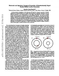
Figure 1.2: Energy bands for copper calculated by Burdick [66] . This calculation used Slater’s APW method with Chodorow’s potential for Cu [67].
In order to use the APW method a form for the spherically symmetric atomic potential is required. This is in general not such a simple requirement as the potential should include the average effect of all the free-electrons in the solid. In order to be self-consistent one needs to solve for the wavefunction, then recalculate the atomic potential, then iterate until there is convergence. This procedure has been adopted [68], however simpler approximations can yield remarkably good results. One can
18 calculate the atomic potential using the Hartree-Fock formalism, and then include the effect of the plane-wave-like electrons using a much simpler calculation of the wavefunction - one that should be valid for those electrons. This procedure was adopted long ago by Chodorow [67] for copper and later used by Burdick to calculate the band structure - as shown in figure 1.2. Despite the age of this calculation it compares very well to more recent calculations [69]. In the early days of computing great efforts were taken to optimise code to be able to do these calculations at all, but now these calculations can be done in seconds on a desktop personal computer. There are an enormous number of variations on the theme of augmented plane waves - Loucks made the pertinent, if somewhat politically incorrect comment on this diversity: “As with women, however, it is far easier to give descriptions than to give useful advice on how to choose one” [70].
1.2.2
Pseudo-potentials
Plane waves are a slowly converging basis in regions where the potential is deep, namely close to the nucleus. An alternative to modifying the basis to improve convergence, is to modify the potential. A pseudo-potential is a potential which will allow a plane wave basis to converge rapidly, yet yield the same band structure as a more elaborate calculation on the true potential. The idea is motivated by the fact that many materials, such as simple metals, noble metals, and semiconductors, are nearly free-electron-like. One example of a pseudo-potential is a muffin-tin potential with a low potential cut off, under which the atomic potential is approximated by a constant. This type of pseudo-potential is motivated by the observation that the details of the deep potential very close to the nucleus should not severely affect the wavefunction at energies where the band structure is calculated. The pseudo-potentials are often very weak compared to the true potential, and particularly good results can be obtained for simple metals and semiconductors. In order to describe transition metals one can use a hybrid basis by adding a TB orbitals to represent the d -bands. This type of approach will be discussed further in relation to the KKR method (section 1.2.3). The reason the pseudo-potential method can be so effective for some systems can be understood by examination of the orthogonalised plane wave (OPW) method. The
19 difficulty with the true potential is that it is very deep, and when the wavefunction is in this region it must oscillate rapidly to reflect the increase in kinetic energy. The OPW method avoids this problem by defining an OPW to be a sum of a plane wave with wave vector, k, and a sum of core levels at the same wave vector, φk = eik.r +
�
Ai ψki (r)
(1.1)
i
where the sum over i is over all the core electronic states. The constants, Ai , are chosen such that the OPW is orthogonal to all the core levels. In terms of this basis we need only expand in a few OPWs as the oscillation at low potentials is built into the basis from the outset. This leads to the idea of a pseudo-potential as this orthogonalisation procedure can be reinterpreted as simply using the plane wave part of the OPW as a basis in a new ‘effective’ Schr¨odinger equation. The difference between the actual Hamiltonian and the effective one removes the deep core part of the potential and makes plane waves a rapidly convergent basis. A disadvantage of this approach is the difficulty in modeling effects where it is essential that the wavefunction takes its correct form near the nucleus, for example for spin-orbit effects. One can account for this by introducing a scaling parameter which may however be difficult to determine in general.
1.2.3
Korringa-Kohn-Rostoker technique
The Korringa-Kohn-Rostoker (KKR) technique was developed first by Korringa [71], and then later from a different point of view by Kohn and Rostoker [72]. The method is an application of multiple scattering theory to electron waves in periodic systems. It can be formulated in terms of Green’s functions, or in scattering theory terminology - the phase shifts of partial waves. Pioneering work investigating hybrid basis sets as a description for transition metals clarified an important connection between TB and KKR. This connection, in part, justifies the TB method and will be discussed further in section 1.3.2. The power of the KKR method derives from its ability to include the effect of the crystal geometry exactly, and in a way which is separated from the particular form of the lattice potential. A spherically symmetric atomic potential is considered that
20 extends to a radius that falls just within the Wigner-Seitz polyhedron. Outside the sphere the potential it is assumed constant - set to zero for convenience. The electrons are free between the spheres, and one can consider the spheres acting to scatter these free electrons. The effect of the scattering can be incorporated into boundary conditions for the wavefunction on the surface of the sphere. Bloch’s theorem determines how the geometrical arrangement of the spheres influences the boundary conditions. This information is contained in the structure constants and have been calculated for various crystal structures in the literature [73]. It then remains to solve the Schr¨odinger equation within the spheres subject to the boundary conditions. The assumed spherical symmetry of the potential allows one to expand the wavefunction in spherical harmonics inside the sphere, which are smoothly connected to Bessel functions outside the sphere. One can express the phase shift, which determines the form of the wavefunction outside the sphere, entirely in terms of the form for the wavefunction inside the sphere [74]. The basis used inside the sphere determines the form for the phase shift, and hence the dispersion relations. If one uses Bessel functions that have been orthogonalised to core states for the basis functions, (along the lines of OPW) then the phase shift contains two terms. The first corresponds to a pseudo-potential calculation as one might expect. The second is usually negligible compared to the first but contains a denominator such that it becomes dominant at a certain energy. This term corresponds to a virtual resonance and is responsible for the d -bands . This explains why non-hybrid pseudo-potential methods are poor at describing transition metals as they neglect this resonance.
1.2.4
Spin dependent electronic structure
The total potential energy in a system is a function of the electronic number density, and therefore depends upon the wavefunction. In order for a band structure calculation to be self-consistent one must iteratively recalculate the wavefunction and potential until they agree within some tolerance. The functional form for the one-electron potential can be derived from the Hartree-Fock approximation. It consists of the periodic lattice potential (electron-ion), the coulomb interaction between
21 electrons, and the exchange interaction. The exchange interaction is a Coulomb-like potential that acts between electrons of the same spin only. It is a consequence of the Coulomb interaction acting on a wavefunction that is antisymmetric - and therefore contains inherent correlations. The Hartree-Fock potential is based upon the simplest antisymmetric wavefunction one can construct from the one-electron wavefunctions. However the form the total wavefunction may take to minimise the ground state energy is not known in advance. Density functional theory (DFT) reformulates the problem in terms of the electronic number density. It was shown by Kohn that the ground state energy is a unique functional of the electronic density [75], but the function is not known and must be approximated. Often a n1/3 local density approximation (LDA) is used for exchange, or more elaborate conjugate gradient approximations (CGAs). In actual implementation DFT changes the difficulty from not knowing how to construct the true many-body wavefunction to not knowing what the universal functional is. It is the exchange interaction that is responsible for ferromagnetism in the transition metals. The exchange term in ferromagnetic materials favours parallel alignment of spins. There is a simple argument due to Stoner that explains the ferromagnetism of the transition metals. The exchange interaction gives an energy penalty for electrons to have opposite spins. If only the exchange interaction mattered then a ferromagnet would be entirely polarised. However, to do this costs a great deal of energy; the Pauli exclusion principle demands electrons must be added at the Fermi energy, which becomes increasingly large as more electrons are added. In transition metals there is a large DOS associated with the d -band near the Fermi energy, which means that many electrons may be added into the same spin with little additional energy cost. Ferromagnetism is the result of a battle between reducing correlation energies due to exchange, and the price in kinetic energy implied by the Pauli principle in aligning spins. A fully self-consistent electronic structure calculation including exchange can predict the ground state electronic structure and magnetic moment of ferromagnetic materials. Figure 1.3 shows a schematic spin-dependent DOS of a transition metal. The d band is spin-split by the exchange energy, J, and as a result there is a net imbalance
22 of electron spin. This imbalance corresponds to a magnetic moment. The spins that are aligned with the magnetisation are labeled as majority electrons, and the spins in the opposite direction are minority electrons. The magnetic effect of primary interest in this thesis is the fact that the electronic structure at the Fermi energy is highly spin-dependent in a ferromagnetic system, and this leads to spin-dependent transport.
g(E)
g(E)
EF
EF
E
E
These aspects will be discussed further throughout this thesis.
(a) Parramagnetic state.
(b) Ferromagnetic state.
Figure 1.3: An illustrative spin-dependant electronic structure for a ferromagnetic transition metal.
1.3 1.3.1
Tight-binding Formalism
The band structure techniques that have been discussed thus far enable the calculation of the one-electron dispersion relations for periodic systems. These methods derive the band structure from knowledge of the atomic potentials and the crystal structure. The tight-binding (TB) method may also be used in this way, but its true power lies in its use as an interpolation method. TB, or linear combination of atomic orbitals (LCAO), makes use of atomic-like orbitals as a basis in which to expand the wavefunction. This proves particularly valid for the resonant d -bands of transition
23 metals, but for some systems – such as simple metals – a TB basis gives a relatively poor description. However TB also has several advantages over alternative methods. APW methods generally do not give good descriptions of semiconductors; whereas a relatively simple TB model can describe the essential features of a semiconductor, such as the band gap, even if it is amorphous. The Hamiltonian is almost diagonal in the real space basis which makes computation rapid and many atoms may be considered. The localised basis is also well suited to examining the effects of perturbations in the crystal structure such as vacancies or surfaces. The TB method will now be introduced in its most general form, before approximations are made to allow further progress. The TB wavefunction is expanded in the following way, Ψ (r) =
�
aα φα (r − rj )
(1.2)
αj
where the sum α runs over a set of atomic-like orbitals centred at rj , and the aα are complex amplitudes associated with each orbital. It is important to appreciate that the φα (r − rj ) are rarely actual atomic orbitals; instead they are atomic-like functions centred on a particular site. If this wavefunction is used in conjunction with a one-electron Hamiltonian the following TB Schr¨odinger equation results, �
Hαjα� j � aα� j � = E
�
α� j �
Sαjα� j � aα� j �
(1.3)
α� j �
where the Hαjα� j � are Hamiltonian matrix elements between the orbitals and are defined as:
� Hαjα� j � =
φ∗αj (r − rj ) H (r) φα� j � (r − rj� ) d3 r
and the overlap matrix, Sαjα� j � , is defined by: � � � Sαjα j = φ∗αj (r − rj ) φα� j � (r − rj� ) d3 r
(1.4)
(1.5)
and represents the degree to which the the orbitals overlap. One can write the total potential of the lattice as a sum of atomic potentials so that the Hamiltonian may be expressed as, H (r) = −∇2 +
� β
Vβ (r − rj )
(1.6)
24 where the sum over β is over localised atomic potentials centred at rj� , and atomic Rydberg units have been used (section 3.3.4). The sum over Hamiltonian matrix elements in equation 1.3 can be decomposed in the following way, � α� j �
Hαjα� j � aα� j � =
�
Sαjα� j � 0α� j � aα� j � +
α� j �
�
Vαjα� j � β aα� j �
(1.7)
α� j � β
where 0α� j � is the result of the kinetic energy operator on the orbital and can be thought of as a site energy - although for d -bands it represents a resonance energy. Vαjα� j � β is the hopping matrix with elements between an orbital, α, on site j and an orbital, α� , on site j � via an atomic potential β. The hopping matrix is almost diagonal as only elements with some overlap of atomic potential and orbital wavefunction are significant. Typically only nearest or next nearest neighbours contribute. If one can construct a fairly localised orthogonal basis then the overlap matrix simplifies to the identity matrix. In general the hopping matrix involves three-centre integrals; namely an orbital at one site, a potential at another site, and a final orbital at a third site. An important simplification can be made by observing that terms with the potential and one orbital on the same site, and a second orbital on a neighbouring site are much more significant. If one neglects the other terms then these two simplifications together are known as the orthogonal two-centre TB approximation, and result in the following TB Schr¨odinger equation,
0αj aαj +
�
Vαjα� j � aα� j � = Eaαj
(1.8)
nn α� j �
where nn indicates a sum over nearest neighbours. The band structure can be calculated easily from such a model if the hopping matrix and site energies are known. In Slater and Koster’s influential paper [76] they describe how one can use the TB method as a very useful interpolation scheme. If one can express the TB band structure in terms of a small number of parameters, then these can be adjusted as fitting parameters in order that the TB band structure agrees with more accurate calculations at particular points of high symmetry. Such a TB model should provide a good interpolation away from these symmetry points. In order for this to be a viable scheme then the number of free parameters must be kept to a minimum. In their paper they made the transformation from atomic orbitals to L¨owdin functions;
25 this slight of hand left the symmetries of the orbitals unchanged but made sure that Bloch sums constructed from this new basis were orthogonal to each other. As the symmetries of the L¨owdin functions are the same as for the orbitals it is useful to think of the basis functions as orbitals in discussing overlaps and hopping matrix elements. The hopping matrix elements are expressed in terms of direction cosines and a small set of parameters. For s-, p- and d-orbitals there are only 10 of these parameters representing overlaps of the various orbitals in certain orientations. In this way the dependence on crystal structure is separated from the problem - although in general the matrix elements can depend on separation in a complicated way. The expressions are shown in table 1.1; the direction cosines l, m, and n refer to the x, y, and z directions respectively. Subsequently these arguments were extended to arbitrary angular momentum orbitals [77]. Figure 1.4 shows three orbital matrix elements schematically. The ssσ matrix element is spherically symmetric, hence there are no direction cosines in its angular dependence. For p- and d -orbitals however there is angular dependence because of the symmetry of these orbitals. A spσ and a pdσ matrix element is also shown in the figure. These overlaps have an additional parity effect associated with the sign of the lobes. An s-p matrix element going in the positive x direction, is the negative of a p-s matrix element in the positive x direction. These parity factors must be included correctly otherwise it leads to a non-Hermitian Hamiltonian. The advantage of a TB description is its ability to demonstrate the physics of electronic structure within a relatively simple model. The details of the electronic structure are contained in a small set of parameters which can be extracted from fits to other band structure calculations. Alternatively one can calculate the TB parameters directly using DFT for example [78, 79]. TB allows one to explore how perturbations affect the electronic structure, such as additional interactions like electron-electron or electron-phonon [80, 81], or structural changes which can be very difficult to incorporate into other methods.
Table 1.1: Slater and Koster’s table of the angular dependance of interatomic hopping matrix elements as a function of the direction cosines, l, m, and n (from left to right orbital) [76]. All other matrix elements are found by permuting the indices.
Vs,s = Vssσ Vs,x = lVspσ Vx,x = l2 Vppσ + (1 − l2 )Vppπ Vx,y = lmVppσ − lmVppπ Vx,z = lnVppσ − lnVppπ Vs,xy = 31/2 lmVsdσ Vs,x2 −y2 = 12 31/2 (l2 − m2 )Vsdσ Vs,3z2 −r2 = [n2 − 12 (l2 + m2 )]Vsdσ Vx,xy = 31/2 l2 mVpdσ + m(1 − 2l2 )Vpdπ Vx,yz = 31/2 lmnVpdσ − 2lmnVpdπ Vx,zx = 31/2 l2 nVpdσ + n(1 − 2l2 )Vpdπ Vx,x2 −y2 = 12 31/2 l(l2 − m2 )Vpdσ + l(1 − l2 + m2 )Vpdπ Vy,x2 −y2 = 12 31/2 l(l2 − m2 )Vpdσ − m(1 − l2 + m2 )Vpdπ Vz,x2 −y2 = 12 31/2 l(l2 − m2 )Vpdσ − n(1 − l2 + m2 )Vpdπ Vx,3z2 −r2 = l[n2 − 12 (l2 + m2 )]Vpdσ − 31/2 ln2 Vpdπ Vy,3z2 −r2 = m[n2 − 12 (l2 + m2 )]Vpdσ − 31/2 mn2 Vpdπ Vx,3z2 −r2 = l[n2 − 12 (l2 + m2 )]Vpdσ − 31/2 ln2 Vpdπ Vxy,xy = 3l2 m2 Vddσ + (l2 + m2 − 4l2 m2 )Vddπ + (n2 + l2 m2 )Vddδ Vxy,yz = 3lm2 nVddσ + ln(1 − 4m2 )Vddπ + ln(m2 − 1)Vddδ Vxy,zx = 3l2 mnVddσ + mn(1 − 4l2 )Vddπ + mn(l2 − 1)Vddδ Vxy,x2 −y2 = 32 lm(l2 − m2 )Vddσ + 2lm(m2 − l2 )Vddπ + 12 lm(l2 − m2 )Vddδ Vyz,x2 −y2 = 32 mn(l2 − m2 )Vddσ − mn[1 + 2(l2 − m2 )]Vddπ + mn[1 + 12 (l2 − m2 )]Vddδ Vzx,x2 −y2 = 32 nl(l2 − m2 )Vddσ + nl[1 − 2(l2 − m2 )]Vddπ − nl[1 − 12 (l2 − m2 )]Vddδ Vxy,3z2 −r2 = 31/2 lm[n2 − 12 (l2 + m2 )]Vddσ − 31/2 2lmn2 Vddπ + 12 31/2 lm(1 + n2 )Vddδ Vyz,3z2 −r2 = 31/2 mn[n2 − 12 (l2 + m2 )]Vddσ + 31/2 mn(l2 + m2 − n2 )Vddπ + 12 31/2 mn(l2 + m2 )Vddδ Vzx,3z2 −r2 = 31/2 nl[n2 − 12 (l2 + m2 )]Vddσ + 31/2 nl(l2 + m2 − n2 )Vddπ + 12 31/2 nl(l2 + m2 )Vddδ 1 2 Vx2 −y2 ,x2 −y2 = 34 (l2 − m2 )Vddσ + [l2 + m2 − (l2 − m2 )]Vddπ + [n2 + 24 (l − m2 )]Vddδ 1 1/2 2 1 2 1 1/2 2 1/2 2 2 2 Vx2 −y2 ,3z2 −r2 = 2 3 [n − 2 (l + m )]Vddσ + 3 n (m − l )]Vddπ + 4 3 (1 + n2 )(l2 − m2 )Vddδ V3z2 −r2 ,3z2 −r2 = [n2 − 12 (l2 + m2 )]2 Vddσ + 3n2 (m2 + l2 )]Vddπ + 34 (l2 + m2 )2 Vddδ 26
27
Vssσ
Vspσ
Vpdσ Figure 1.4: Illustration of typical matrix elements in tight-binding.
1.3.2
Justification of tight-binding
Tight-binding can describe a great deal of the physics of a wide variety of systems. Its short ranged nature makes it particularly amenable to computation, and large systems can be studied easily. It is perhaps, on first inspection, somewhat surprising that a description of electronic structure based upon a spatially localised basis should be a valid one; particularly knowing that the nature of electronic states in many metals is better described by extended plane waves. However, parameterised TB band structures can reproduce the correct electronic structure of many systems. Important quantities calculated from them, such as group velocities and Fermi energies, are also in good agreement. The d -bands of transition metals are particularly well described by TB, however it is not immediately apparent why this should be the case. The narrow d -bands arise from a virtual resonance as was discussed in section 1.2.3. The consequence of this is that the d -wavefunctions are better described by long tailed Bessel functions rather than short ranged atomic orbitals. Despite this, the KKR formalism may be transformed into a short ranged TB model for the d -bands [74]. This is possible because destructive interference occurs between the tails of Bessel functions originating at distant sites, leaving only contributions from near neighbours to the TB matrix elements.
28 The nearly free electron sp-bands are in general not so well described by TB methods. The work of Heine, Hodges and Mueller for example used a hybrid basis of OPWs and TB orbitals [82, 83, 84]. Such a simple model can describe many features of transition and noble metals. Free electron-like bands can only be described well by TB near the bottom of a band, or just above a d -band to which it is hybridised. One would therefore expect very poor band structures for simple metals, and fairly poor band structures for almost everything else. However Papaconstantopoulos has shown that when using the TB method as an interpolation scheme, and viewing the parameters as adjustable fitting parameters, very good agreement can be obtained. Qualitatively one can understand the success of TB by analogy with the pseudopotential method (section 1.2.2). A pseudo-potential is defined such that a plane wave basis generates the same band structure as would be calculated using the true potential with a more suitable basis - such as OPWs. Alternatively, the opposite could be done: creating an effective Hamiltonian for the orbital part of the OPW. The fact that parameterised TB band structures can agree quite well with plane wave based methods seems to suggest that such a transformation is possible. The variational principle also comes to the aid of a TB method, as any error made in the wavefunction will lead to only second order error in the energy. Electronic transport is the principle concern throughout this thesis, and therefore it is the electronic structure close to the Fermi energy that is most important. For transition and noble metals TB is a particularly good approximation as the Fermi energy either lies inside the d -bands, or just above them.
1.3.3
Band structure calculations
Table 1.1 contains the orientation dependence of the hopping matrix elements and involves ten parameters, which if known as a function of orbital separation, would allow one to calculate the electronic structure of a material in any crystal structure - or even in an amorphous phase. Two types of approach have developed faced with this possibility; one can attempt to describe many elements with just a few ‘universal’ parameters, or one can calculate different parameters for each element in order to improve the band structures. In this section both types of approach will be
29 discussed. Harrison’s book on the electronic structure of solids [85] presents the results of a research effort aimed at tabulating TB parameters for most of the periodic table. The culmination of this work was the solid state table of the elements, which contains parameterisations for all elements between Helium and Americium with varying degrees of accuracy. The parameters determined by Harrison are based upon simple chemical bonding principles, and comparisons of TB band structures with those calculated using muffin-tin orbital [86] and pseudopotential approaches. The aim was to describe as much of the periodic table as is possible with as few parameters as is possible. Simple arguments based upon muffin-tin orbitals (or alternatively Bessel functions in KKR theory) enable the separation dependence of the hopping matrix elements to be factored out of the problem. One considers the overlap of a muffin-tin orbital (MTO) on a site, with the tail of a MTO from a neighbouring site. This leads to a separation dependence for the hopping matrix element of the following form [79, 82], �
Vll� m = Cll� m d(−l+l +1)
(1.9)
where l and l� are the angular momenta of the two orbitals, m represents the direction the orbitals are coupled in, and d is the separation. However Harrison found that for s-s matrix elements the dependence did not agree with free-electron estimates and so the dependence was adapted in the following way; s-s, s-p and p-p matrix elements 7
decay as 1/d2 ; s-d and p-d matrix elements decay as 1/d 2 ; and d-d matrix elements decay as 1/d5 . These simple approximations can lead to quite reasonable predictions. However if the separation between orbitals varies by a small amount almost any variation looks linear and the argument based on the tails of MTOs is irrelevant. If one uses this separation dependence the s and p-orbital matrix elements can be expressed in terms of universal constants valid for any element. The d matrix elements required for transition metals however depend on the nature of the d-resonance and so an additional parameter, the radius of the d-resonance, is required for each element. These very simple ideas together with a relatively small set of parameters can be used to sketch out the important features in the electronic structure of almost any element. Figure 1.5 shows how reasonable such a calculation for Ni can be with a
30
Figure 1.5: (a) The band structure of Ni calculated with Harrison’s solid state table of the elements. (b) An independent calculation of the band structure using the APW method [87]. [Taken from reference [85].]
comparison to an APW calculation. Although they differ by a small scale factor, the main features are clearly present in both calculations. This illustrates the ability of very simple TB models to correctly describe the band structure, and they can do so even when long range order is absent. There are good reasons to seek a TB parameterisation valid for all elements using as few parameters as possible. Such a model will be a useful tool enabling better understanding of how electronic structure arises when atoms condense into a solid. However, in this kind of approach there must be a compromise between a precise description of electronic structure and the number of free parameters. An alternative approach is to find the best TB parameterisation possible by having a separate set of parameters for each element. The hopping matrix elements, and overlap matrix elements in a non-orthogonal representation, can be seen as adjustable parameters which should be determined by a fit to more accurate band structure calculations. Perhaps the best and most complete parameterisation of this kind has been carried
31 out at the Naval Research Laboratories (NRL) [88]. TB parameters are used to fit self-consistent scalar relativistic APW band structure calculations at several different lattice constants and different crystal structures. The Slater-Koster orientation dependence is utilised to reduce the number of parameters and a least squares fitting procedure is used. Typical root-mean-square discrepancies in the energy throughout the Brillouin zone are of the order 1/20eV. The separation dependence of each parameter for any crystal structure is then fit with an empirical functional form rather than the simple form suggested by MTOs or KKR, S (r) = (a + br) e−c r H(r) 2
(1.10)
where H(r) is a Heaviside function that cuts off the matrix elements at separations greater than 16 Bohr radii. The first term can be a polynomial of any order, but typically a first or second order polynomial will accurately describe the dependence on crystal volume. Total energy calculations can be performed using these parameters which correctly predict the ground state crystal structure and lattice constants for many elements. Due to the relative computational efficiency of the TB method, more complicated total energy problems can be tackled than would be possible using other methods. The ground state of manganese, α-Mn, for example has a very complicated crystal structure with 29 atoms in its unit cell. The parameterised TB model correctly predicts the ground state crystal structure of manganese [89], and the pressure at which the β-Mn structure should be preferential is in good agreement with experiment. Papaconstantopoulos has tabulated the results of the NRL TB parameterisations in his book [55]. Very good equilibrium band structures can be generated using the simple two-centre and orthogonal TB scheme, while for volume dependent total energy calculations a non-orthogonal representation produces better results. Figure 1.6 shows a recent TB paramaterisation for Ge in the diamond crystal structure together with a comparison to an APW method. The top panel is a parameterisation using a basis of four orbitals; 1s and 3p. The bottom panel used 5d-orbitals in addition. The agreement is very good for both models, but the four-orbital model agrees less well at very high energies. The NRL TB method has also been applied to parameterise magnetic materials. The band structure in this case is fit to self-consistent APW calculations
32 that include exchange and correlation effects [90].
Figure 1.6: Tight-binding parameterisation for Ge [taken from [91]]. The solid lines represent the TB band structures and the symbols are the results of an APW calculation. Top panel - sp3 basis. Bottom panel - sp3 d5 basis.
The assumption of a perfect periodic crystal is vital to many methods used to calculate electronic structure. There are many situations however where this is far from the case, for example at a surface or at an interface in a multilayer. In such cases we can no longer talk of band structure, yet there must still be electronic structure. Understanding the electronic structure at surfaces is important in many situations; for example scanning tunneling microscopy (STM) or spectroscopy (STS), and for effects in magnetic materials where the moments can be enhanced or degraded near a surface (magnetic dead layers [92]). There are far fewer methods suited to calculation of electronic structure in such situations and TB is frequently employed for this purpose [92, 93, 94]. Structurally disordered systems, such as materials like a-Si, often have interesting electronic structure and are frequently investigated with TB models [56]. The application of an empirical TB scheme is not straightforward even for single
33 elements. The fitting of the separation dependence of matrix elements can be highly non-linear and great care must be taken to ensure the results are reasonable. Beyond single element calculations effects such as charge transfer in alloy systems can be difficult to account for accurately using an empirical method. The development of DFT together with huge increases in computational power over the last few decades presents another possible approach to TB: one can directly calculate the matrix elements from first principles. Such approaches have been applied with success to some systems such as Si and C [78], however, transition metals, with the need to accurately represent the d -bands, prove to be difficult to handle. A first principles approach is only really justified if empirical methods can not be used as it requires a great deal of computational effort to calculate the matrix elements.
1.4
Summary
In this chapter electronic structure has been discussed in some detail, with particular emphasis on the tight-binding method. This model of electronic structure is used extensively in this work and it is important to understand its connections with other techniques. The following chapter is concerned with electronic transport where there are many important connections with ideas discussed in this chapter.
34
Chapter 2 Electronic transport 2.1
Introduction
The purpose of this chapter is to provide a detailed discussion of electronic transport, with particular emphasis on concepts and techniques relevant for complex nanoscale systems. A number of important ideas will be discussed, including the role of the electrochemical potential, interface resistances and quantum interference effects. Several important methods will also be described such as the Boltzmann, Kubo, and Landauer-B¨ uttiker formalisms. This chapter will provide a broad foundation onto which the EOM method that is the central part of this work will be built upon. The EOM method will be introduced in the next chapter. In the early part of the twentieth century, new technological developments paved the way for electrical transport measurements on a wide range of novel systems. Innovations such as helium temperature cryogenics, and device fabrication techniques such as sputtering [95], enabled measurements to be made on increasingly small temperature-, and length-scales. Since then, and to this day, such measurements have revealed a plethora of interesting transport effects. A theoretical understanding of many of these phenomena required the development of new methods, while in other situations judicious approximations could be used with already existing techniques. Throughout this work we will be concerned with the D.C. electrical conductance of complex nanoscale devices. We shall be interested particularly in systems which have spin-dependent electronic structure. Such systems are commonly considered in the field of spintronics, a prime example being the current-perpendicular-to-plane giant magnetoresistance (CPP GMR) effect. Specifically we will concentrate on devices for
35 which linear response is appropriate. Many systems with technological applications fall into this category, as the desire is for low power consuming devices. Exceptions to this include transistor devices for example - where space charge can be important. For most metallic devices linear response is valid over all potential differences of practical interest - often devices would be destroyed through heating before nonOhmic behaviour is observed. The calculation of the D.C. conductance, and its dependence on various factors, such as temperature and applied magnetic fields, is an important problem. There are numerous theoretical methods that are applied frequently in the literature to understand transport in complex systems. The accurate representation of the electronic structure can often be of central importance. Electronic transport is a vast subject, and it has naturally fragmented over the years into numerous more focussed areas of research; semiconductor physics, mesoscopics and spintronics for example. There are some basic concepts that are relevant to all areas of electronic transport - the electrochemical potential for instance. However there are also ideas, such as spin-polarised currents, which apply more specifically and can involve additional issues. In the first part of this chapter important basic concepts relevant to the kinds of system that will be the focus of this thesis are introduced. The role of interfaces in inhomogeneous structures, and the additional effects associated with the introduction of spin-dependent electronic structures will be discussed. The remainder of the chapter will present several important methods commonly used to calculate transport properties in complex systems. In discussing these formalisms particular attention will be paid to how what is calculated relates to a measurement of conductance. The advantages and disadvantages of each approach will be highlighted, and it will become clear that these methods are often suited to a particular class of problem. A discussion of these methods will clarify the nature and importance of the technique introduced in the next chapter.
36
2.2 2.2.1
General concepts The electrochemical potential
The D.C. electrical conductance of a system, G, is defined in terms of the potential difference, V , and the electric current, I, in the familiar way, G=
I . V
(2.1)
Although this a very well known equation it is worth including as it is so fundamental to this work. The conductance, or a geometrically related quantity such as resistivity, is the objective of the methods that will be presented in this chapter - although often they can also be used to calculate many other transport coefficients. Prior to a discussion of some of these important techniques, it is crucial to discuss the fundamental driving forces for electric current. Electronic transport is often discussed in terms of electrostatic fields, particularly in metals [96], however the electrochemical (EC) potential, Φ, is the true driving force for electrons in the absence of magnetic fields. It is defined in terms of the electrostatic potential, φ, and the chemical potential energy, μ, in the following way, 1 Φ (r) = φ (r) − μ (r) . e
(2.2)
The chemical potential is related to the electronic number density in a system, and the electrostatic potential is due to electric fields - both internal and externally applied. The two are self-consistently related; number density variation gives rise to space charge, and this determines the electrostatic potential through Poisson’s equation. The EC potential is perhaps a more familiar concept in semiconductor physics, where the combination of electrostatic and chemical potentials can give rise to dramatic effects. In a macroscopically homogenous system in equilibrium, the chemical potential is constant throughout and is known as the Fermi energy, EF . It is useful to define the Fermi energy in terms of the electronic DOS, g (E), in the following way, � ∞ g (E) f (E − EF ) dE = n0 0
(2.3)
37 where n0 is the constant electron number density in the system, and f is the Fermi function. In general the DOS is spin-dependent, and one can define a separate chemical potential for each spin eigenstate. In equilibrium the chemical potential for each spin is equal, but this is not necessarily the case if a non-equilibrium current flows. In a system driven out of equilibrium there may be spatial variation in the chemical potential due to a varying electronic number density, n (r). This statement may be an oversimplification, as in general the definition of a local number density is not straightforward. A suitable local average over an appropriate length-scale must be used - the mean-free-path for example. Given this proviso, the non-equilibrium change in chemical potential, δμ (r), can be defined in the following way, � ∞ g (E) f (E − EF − δμ (r)) dE = n (r) .
(2.4)
0
This definition assumes electrons are sufficiently close to equilibrium that a FermiDirac distribution describes them correctly. This is always the case for a sufficiently small potential difference, and for larger potentials there must be sufficient inelastic scattering to allow the ‘hot’ electrons to give up their excess energy to the lattice. If one assumes zero temperature, and small chemical potential variations, one may expand equation 2.4 in the following way, � ∞ � ∞ g (E) f (E − EF ) dE + δμ (r) g (E) δ (E − EF ) dE = n (r) 0
(2.5a)
0
n0 + δμ (r) g (EF ) = n (r) .
(2.5b)
The relationship between variations of chemical potential and variations of the electronic number density can be identified as, δμ (r) =
δn (r) g (EF )
(2.6)
where δn (r) = n (r) − n0 . Electric fields and variations of chemical potential can give rise to electric currents. For small EC potential differences the current response is linear, namely the current is directly proportional to the applied potential. In linear response the precise composition of the EC potential is irrelevant, and chemical potentials are as effective at driving current as electrostatic potentials. This equivalence is only valid in linear response as the roles of electrostatic and chemical potentials are fundamentally
38 different - the former can accelerate electrons, while the latter cannot. An example indicating the self-consistent nature of the EC potential is included in appendix A. In equilibrium when no net current flows, the fluctuating current contributions from chemical potential gradients must balance equally those from electrostatic potential gradients. This implies an important connection between the diffusive and conductive properties of a system. If we consider a macroscopically homogeneous material characterised by a constant local conductivity, σ, the relevant linear response transport equation is simply, 1 J = σ∇Φ = σ∇φ − σ ∇μ e
(2.7)
where J is the electric current density. A diffusion coefficient, D, for a homogeneous system is defined in terms of the transport equation, JD = −D∇n
(2.8)
where JD is a diffusive particle current. This equation can be expressed in a form that allows comparison with equation 2.7, 1 J = −e2 g (EF ) D ∇μ . e
(2.9)
Hence one can make the following connection between the diffusion coefficient and the conductivity for a homogeneous system, σ = e2 g (EF ) D .
(2.10)
This is known in classical physics as the Einstein relation, and may be generalised to energy dependent diffusion coefficients and conductivities. The relation is also valid in the case when conductivities are non-local [97]. Similar arguments can be used to obtain the Einstein relation for non-degenerate semiconductor systems, where (kB T )−1 replaces the DOS.
2.2.2
Quantum-mechanical effects
Electron dynamics are governed by the Schr¨odinger equation, and to fully understand electron transport one would in general need to solve a complex non-equilibrium
39 many-body problem. This can only be attempted for very simple systems, and even then employing approximations. However it is often the case that a one-electron picture can capture most of the important physics. In many cases one can regard the electrons as non-interacting; each moving in the potential due to the electric field, in addition to the self-consistent periodic potential. It may seem unreasonable that such a simple approximation for non-equilibrium transport problems should be used. However, Fermi liquid theory provides some justification for this [98]; the one-electron dispersion relations and DOS can be considered to be that of weakly interacting quasiparticles rather than electrons. Most materials relevant for devices, such as metals and semiconductors, are good Fermi liquids however there are some exceptions to this that require alternative approximations such as heavy fermion systems and L¨ uttinger liquids for example. Such systems are beyond the scope of this thesis. There are some aspects of electron transport where the quantum-mechanical, wave-like nature of the electron plays a direct role. Weak localisation is one example of such an effect that can be observed in solid state disordered systems. The effect itself is entirely classical and has been observed for light in a disordered medium [99, 100], and even seismic waves in the earth’s crust [101]. It is the quantum-mechanical nature of the electron that makes this effect observable in highly disordered systems, such as amorphous alloyed systems. In a disordered system at zero temperature and magnetic field, electrons scatter through an array of static impurities or defects coherently. There is a definite phase relationship between the wavefunction at any particular point and the source of electrons, which is determined by the scattering properties. Constructive interference between time reversed trajectories leads to a decreased probability of an electron diffusing away from a particular position. This effect leads to an overall reduction in the diffusion coefficient, and a corresponding increase in the resistivity. One can reduce this effect by the application of an agent to destroy the interference. A magnetic field can be used to make the time-reversed path acquire a phase difference, and temperature can be used make time reversed paths incoherent. Spin-orbit has also recently been shown to have an important effect [102]. This can be experimentally investigated by doping a small amount of a strong spin-orbit scatterer into a highly disordered alloy - CaAl:Au for example. This
40 effect will be considered in more detail in chapter 5. In solid state systems which are extremely disordered Anderson localisation can occur, where the diffusion coefficient is reduced to zero. However systems of finite extent attached to conducting leads can still conduct in this localised regime as the wavefunctions are localised over a finite length-scale. In fact there can often be significant fluctuations in |Ψ (r) |2 for a localised wavefunction [103]. At finite temperature there are various mechanisms of electron hopping that can also enable conduction. In calculations of the conductivity of disordered systems it is usually necessary to average over disorder configurations in order to obtain an ensemble average of a quantity of interest. The variations from configuration to configuration can be so significant close to localisation that it is necessary to consider the logarithm of conductance if trying to discern a metal-insulator transition. In inhomogeneous multilayer structures, often a non-equilibrium current is directed through several consecutive planar interfaces. The interference between transmitted and reflected electrons from consecutive interfaces can lead to standing wave effects. This can make the transport properties highly sensitive to the separation between interfaces, and can contribute to non-local and non-additive behaviour of interface resistances. Quantum well states can also be formed in multilayer structures, and are understood in much the same way as is discussed in most elementary quantum mechanics textbooks. The quantum-mechanical nature of the electron can clearly be very important in such systems.
2.2.3
Interface resistance
Many interesting systems are some form of heterostructure, containing more than one type of material. As such they can contain interfaces, and in some cases the electric current flows normal to these interfaces. There are a number of effects that can arise as a consequence of bringing two dissimilar materials together. When a semiconductor is attached to a metal for example, significant charge transfer occurs at the interface in order that a common Fermi energy can be established. This has a profound effect on the electronic structure, and the consequence for transport is that electrons must tunnel through, or pass over, a potential barrier to get into
41 the semiconductor from the metal. We shall be primarily concerned with metallic systems in this work, where interfaces generally do not cause such extreme charge transfer effects - however interface effects can still be very important. With regard to transport, interfaces give rise to two effects of principle concern. Firstly there can be an abrupt change in electronic structure when going from one material into another. Electronic states propagating on one side of an interface may not have corresponding available states on the other side. This means these electrons must be scattered into an available state, or reflected at the interface. This will cause an accumulation of electrons near the interface, and a corresponding drop in EC potential associated with an effective interface resistance. The second effect of concern is structural rearrangement at the interface. In general different materials will have different bulk lattice constants and crystal structures. When two materials are brought together there must be a compromise between the energetically favoured structures for each. Typically this can involve a number of effects: a local change in the crystal structure, strain to be taken up by the lattice or inter-diffusion of atoms from each material for example. These effects tend to increase the resistance close to the interface, and depending on the degree to which the materials are incommensurate can extend some distance away from the interface. If we consider an ideal interface between two perfectly crystalline materials, the interface effect can be interpreted in terms of the band structure. It is the electrons at the Fermi energy that are relevant for transport, and it is useful to consider the projection of the Fermi surface for each material in the direction of the interface. This indicates the allowed values of in plane wave-vector, k� , for each material at the Fermi energy. For a free electron system it is simply a circle of radius, |kF |, although in general it will depend on the orientation of the interface (111 or 100 for example). For values of k� where there is no overlap of the two Fermi-surface projections, electronic states cannot propagate and must be reflected, or transmitted as evanescent states. Where there is overlap, there will be transmission but to determine the magnitude one must consider the details of the electronic structure. Strictly, this argument can only be considered meaningful for a crystalline system - where k� is a conserved quantity. As a very simple example we can consider an interface between two free-electron
42 materials at a potential step, Δ. At the Fermi energy plane waves propagating towards the interface at a given k� will be partially transmitted and partially reflected. One � � can therefore define T k� as the transmission coefficient for electric current. Working in atomic units, where � = 2m = 1, one simply matches up for each k� an approaching 1/2 2 wave of the form eikz z to a transmitted wave ei(kz −Δ) z and a reflected wave of the form e−ikz z . A straightforward calculation gives: �1 � � �1 � � 4 E − k� 2 2 E − k� 2 − Δ 2 T k� = �� �1 � � 1 �2 . E − k� 2 2 + E − k � 2 − Δ 2
(2.11)
Although this is a very simple example, calculations on more complicated electronic structures usually proceed in the same way. With the transmission coefficient in hand, the resistance that arises from an interface may be estimated using the Boltzmann equation [39, 104], or the Landauer formula; both the Landauer and Boltzmann formalisms will be discussed in more detail in this chapter. It is often useful to discuss interface resistances in terms of resistance-area product AR. The Landauer formula implies that interface resistance only varies by an order of magnitude for transmission probabilities between 10% and 90% (as shown in figure 2.1). Therefore typically the interface resistance per spin is in the range 0-5fΩm2 . For comparison, a material with bulk resistivity of 3μΩcm, typical of copper, would need to be about 300 monolayers thick in order to have a similar resistance-area product, AR = ρL. For small inhomogeneous systems, the interface resistance can dominate the transport.
2.2.4
Spin-dependent transport
The electron’s spin is an additional degree of freedom which in many calculations simply adds an innocuous factor of two. For ferromagnetic materials, or heterostructures containing ferromagnetic materials, one must consider the spin explicitly. The rapidly developing field of spintronics is concerned with spin-dependent electronic transport. It has already found many device applications, such as GMR sensors for hard disks and magnetic random access memory (MRAM). There are also numerous potential devices in development, such as spin-FETs and spin-torque devices [105]. Ferromagnetic materials are incorporated in these devices in order to introduce the
43
Figure 2.1: Interface resistance between two free-electron-like materials calculated using the Landauer formula. Incident electrons are assumed to have Fermi wavevector, |kF | = 1010 m−1 . The resistance-area product per spin is plotted as a function of the average reflection coefficient over the Fermi surface.
spin-dependence, and magnetic fields can be applied to modify the transport properties. Ferromagnetic transition metal elements, and their alloys, are frequently used because the electronic structure at the Fermi energy is highly spin-polarised. They also remain ferromagnetic at fairly high temperatures, typically higher than 600K. The Fermi energy in ferromagnetic cobalt for example lies in the middle of the d band for minority carriers, and just above the d -band for the majority. There is a high density of minority electrons with a very low mobility, and a lower density of majority electrons with an almost free-electron-like mobility. These materials are itinerant ferromagnets; it is the electrons that carry the current that also carry part of
44 the magnetisation. This is in contrast to local moment ferromagnetic materials, such as Dy for example, which have a relatively weak spin-polarisation of the conduction electrons due to a Ruderman-Kittel-Kasuya-Yosida (RKKY) interaction [20]. In the absence of spin mixing, through the spin-orbit interaction for example, the conductivity of each spin-channel is additive. This is a simple consequence of imposing the same EC potential difference across the system for each spin. If the conductivity of each spin is different, σ↑ �= σ↓ , it implies the current must be spin-polarised. The conductivity of the minority carriers in ferromagnetic transition metals is often small due to the low mobility of the d -band electrons, and in such cases most of the current is carried by the majority electrons. If a potential difference is applied across a ferromagnet/paramagnet bilayer, a net spin-polarised current can be injected from the ferromagnetic layer. These concepts have important consequences for spintronics and will be discussed further in relation to CPP GMR in chapter 5. Interface effects can be very pronounced for spin-dependent transport. Figure 2.2 shows the result of a calculation performed using the electronic structure of Cu and Co calculated using an APW method [106]. The transmission of Bloch states at various k� is calculated by determining the appropriate one-dimensional potential from the APW calculation. Note that the majority Co matches very well to the Cu leading to good transmission, while the minority Co into Cu is very poor.
2.3
Transport formalisms
In this section a number of important methods that can be used to calculate electrical conductance will be introduced and discussed. In fact many of the techniques that will be mentioned can be used, with minor modification, to calculate other linear response transport coefficients - such as the Hall coefficient, the thermal conductivity or the Seebeck coefficient for example. However the focus here is on electronic transport, and specifically in complex and inhomogeneous systems. The use of Boltzmann-type equations, of which there are very many variations, is discussed first.
45
Figure 2.2: Spin-dependent transmission probabilities for Cu/Co (001). The bottom right panel is split into 4 sections as there are multiple Fermi-surface sheets at a given in plane wave-vector. The four sheets are obtained by reflecting and rotating each quarter into the entire surface Brillouin zone. [Taken from [106]]
2.3.1
Boltzmann equations
Boltzmann equations are used frequently in many areas of science to describe the dynamics of systems containing a large number of particles. Rather than solve for the dynamics of every particle in a system, a statistical approach can be used. The state of the system is defined by a distribution function that specifies the occupation probability of points in phase space. Equations of motion for the distribution functions can be constructed, and then solved employing various approximations. Such equations were originally developed for classical physics, but were quickly extended to deal with quantum systems soon after the development of quantum mechanics. A Boltzmann equation can be used to calculate the linear response D.C. conductivity of a system. The non-equilibrium distribution function (DF) under steady state conditions is required. In steady state the effect of the electric field is balanced by the
46 equilibrating effect of collisions. The DF for electrons can be specified as a function of position and wave vector, f (k, r). The linearised Bloch-Boltzmann equation for elastic scattering determines the DF to first order in the electric field in the following way, v.∇r f (k, r) + � Wk� k f (k� , r) (1 − f (k, r)) − Wkk� f (k, r) (1 − f (k� , r)) dk� = −eE.vδ (E − EF ) (2.12) where v is the group velocity and the scattering probabilities, Wkk� , can evaluated using perturbation theory for example. Additional fields and sources can be added to this equation in order to model a particular system. The delta function on the right hand side of this equation corresponds to the derivative of the Fermi function. The Boltzmann equation in this form assumes the state of a system can be specified in terms of a DF which is real (in the mathematical sense). Such a description cannot account for interference effects that should be present, and would be included if one considered the density matrix for example. Although observable quantities can only depend upon the diagonal elements of the density matrix, the off-diagonal elements can still have important effects. Kohn and Luttinger demonstrated that for a low density of weak scatterers, a solution of the density matrix equation is equivalent to the Boltzmann approach [107]. In fact the Bloch-Boltzmann equation is used in many more general situations, describing the electron-phonon interaction for example [24]. The connection between the density matrix formulation and the Boltzmann equation can be made clear by considering the Wigner distribution function (WDF) [108]. It is defined as a transformation of the density matrix into centre-of-mass coordinates. This permits it to be interpreted as the probability for finding a particle in a particular state, without difficulties arising from the uncertainty principle. It satisfies an equation of the same form as the Boltzmann equation, � � � � q � 2 Im V (q) eiq.r fw k + , R dq = −eE.vφ (k, R) v.∇r fw (k, R) + � 2
(2.13)
where fw (k, R) is the WDF, V (q) is the Fourier transform of the scattering potential, and φ (k, R) is the WDF representation of the derivative of the Fermi function with
47 respect to the Hamiltonian. A useful feature of this expression is the ability to demonstrate that current is divergentless independent of the imposed electric field. One can simply integrate both sides of the equation with respect to k, and then � realise that vfw (k, R) dk is the current density. If a non-self-consistent electric field is imposed, part of the electron density will act to make it consistent - and this density will carry no current. Often the Boltzmann equation is solved using the relaxation time approximation. In general the scattering term could have a complicated form that depends upon the non-equilibrium DF. However if it is assumed that the rate of collisions does not depend upon the form of the DF, one can define a relaxation time, τ (k), characterising the decay of the non-equilibrium DF in the absence of applied fields. This time may be calculated using perturbation theory, or by evaluating the T-matrix for a system. For a simple estimate a first order Born approximation can often be reasonable for weak scatterers. The Bloch-Boltzmann equation in its simplest form assumes free-electron planewave states, and an isotropic relaxation time, τ . This is a reasonable description of a liquid metal for example, where one cannot construct Bloch states. However this simple model is often applied to systems where it is not such a good approximation, but can still semi-quantitatively describe important trends. The conductivity calculated in this way is identical to the Drude result - despite this being based on incorrect assumptions. Such a model, although very simple, can be very useful to examine the effects of inhomogeneities and spatial constrictions on a system. Appropriate boundary conditions can be specified for the DF at interfaces or surfaces. Once the DF is calculated for a given system geometry, the conductivity can be estimated. Often such calculations consider the relaxation time as a parameter, rather than calculating it using perturbation theory. The Fuchs-Sondheimer theory [26] is an application of the Boltzmann equation to study the effect of the mean-free-path on the conductivity of thin films. The simple free-electron model is used, and the mean-free-path is considered as an adjustable parameter that determines the bulk conductivity. As the film thickness decreases, the boundary conditions affect the DF to such an extent that the conductivity is altered
48 from is bulk value. There are numerous related applications of the Boltzmann equation to thin film multilayers. Camley and Barna´s [27] applied the Fuchs-Sondheimer treatment to CIP GMR, by generalising to two spin channels and introducing boundary conditions at the interfaces. In a similar treatment Valet and Fert [30] considered the CPP geometry, and included the effect of spin-relaxation through an adjustable parameter. In applications to inhomogeneous systems such as these one can often take advantage of a particular symmetry to make a problem essentially one-dimensional. These types of calculation can be very useful, however there are some problems. In some situations, particularly in inhomogeneous systems, it is difficult to unambiguously define local relaxation times. A sensible choice is to average over local properties, but the range of averaging must surely be related the local mean-free-path - which is the quantity that one is trying to calculate. In addition, without using the quantum form of the Boltzmann equation effects of interference cannot be included and this is likely to be important for inhomogeneous nanoscale systems. While Boltzman equations can be very useful in some situations they have clear limitations.
2.3.2
The Kubo formula
Kubo formulas refer to a large family of similar equations that relate linear response coefficients to correlation functions. Such formulas were first considered by Green [109] for liquids, and then later by Kubo [31] and Greenwood [32] for electrical conductivity. Perhaps the simplest way to derive the Kubo formula for electrical conductivity is to consider the density matrix, ρ, whose equation of motion is, i�
∂ρ = [H, ρ] ∂t
(2.14)
where H is the Hamiltonian. The Hamiltonian can be split into two parts; H 0 representing the periodic potential together with impurities, and a part representing an externally applied electric field. If the electric field is in the x-direction, and is switched on adiabatically the Hamiltonian takes the following form, H = H 0 + eExe�t .
(2.15)
49 This adiabatic switching on of the electric field ensures there are no transients in the steady state. It also allow one to keep track of terms in the density matrix which are first, second, or nth order in the electric field. Alternatively one can remove transients by allowing a finite coupling to the surroundings [110]. In either case the limit → 0 will eventually be taken. The corresponding linearised density matrix can be expressed as ρ = ρ0 + ρ1 e�t
(2.16)
where ρ0 is the equilibrium density matrix associated with H 0 . If terms to first order in E are retained, and matrix elements between eigenstates that diagonalise the unperturbed Hamiltonian are formed, the density matrix equation simplifies to, i� ρ1nm −
�� � 0 1 0 Hnl = eE[x, ρ0 ]nm . ρlm − ρ1nl Hlm
(2.17)
l
In this expression ρ0 is simply the fermi function, f (H 0 ). The commutator can be expressed in the following way if f (H 0 ) is expanded in powers of the Hamiltonian [108],
� � f (En ) − f (Em ) [x, f H 0 ]nm = i�vnm En − Em
(2.18)
and therefore, ρ1nm =
1 x f (En ) − f (Em ) . eEi�vnm i� + (Em − En ) En − Em
After some simplification and taking the limit → 0 one obtains,
f (En ) − f (Em ) f (En ) − f (Em ) 1 x . −i ρnm = πe�Evnm δ (Em − En ) En − Em (En − Em )2
(2.19)
(2.20)
One of the Fermi functions in the real part of the bracketed term can be expanded in terms of the other. The produces a delta function at the Fermi energy, and the non-equilibrium part of the density matrix is given by,
f (En ) − f (Em ) 1 x . ρnm = πe�Evnm δ (En − EF ) δ (Em − EF ) − i (En − Em )2
(2.21)
It is simple show that the equilibrium density matrix gives rise to no net current, and therefore the current in the x-direction is given by, jx =
� 2e � Re Trv x ρ1 Ω
(2.22)
50 where Ω is the volume, and a factor of 2 is introduced for spin. The imaginary term in the brackets of equation 2.21 corresponds to a non-current-carrying density. It is proportional to matrix elements between states above and below the Fermi energy, and is related to the dielectric properties of the system [110]. The conductivity is given by, σxx
2πe2 � � x x = v v δ (En − EF ) δ (Em − EF ) Ω nm nm mn
(2.23)
and this is the Kubo-Greenwood formula for the D.C. electrical conductivity. Similar arguments can be used to obtain other linear response coefficients, such as the Hall coefficient [111] for example. Originally Kubo derived this considering the absorbtion from an A.C. electromagnetic field, and taking the limit of frequency tending to zero. The assumption of a uniform electric field in the derivation of the Kubo formula has important consequences that are often ignored. The right hand side of equation 2.21 clearly demonstrates the existence of non-equilibrium contributions to the number density that carry no current. Associated with this density are variations in chemical potential, which should be self-consistently related to the electric field. If a non-self-consistent electric field is imposed this density will act as an effective field that would not be present if one had started with the self-consistent electric field [112]. Clearly the Kubo formula must be applied with some reservations for inhomogeneous systems, where density variations may be significant. The Kubo formula can be expressed in terms of the one-body Green’s function of a system. One considers equation 2.23 with the velocity matrix elements written out in full; products of eigenstates and delta functions can then be identified as Green’s functions [113], σxx�
2πe2 � = Ω
� �
d d ImG (r, r� , EF ) � ImG (r� , r, EF ) drdr� . dx dx
(2.24)
This may be generalised easily to the full tensor, σαβ . The advantage of specifying the Kubo formula in terms of Green’s functions is that manipulations may be carried out which are independent of the boundary conditions. The full Green’s function for a system may be determined using any means, and subsequently used to calculate the conductivity. The numerical evaluation of the Kubo formula is not straightforward, even for
51 fairly simple systems. The conductivity is defined for an infinite system, where the spacing between energy levels tends to zero. In practice a finite system can be considered if the states are broadened in energy, by coupling to leads or to a temperature bath. Alternatively the delta functions that appear in the Kubo formula can be broadened so that enough electronic states are present. However the delta functions must not be broadened too much in comparison with �/τ , where τ is the lifetime of a Bloch state, otherwise the value of the conductivity becomes determined by the width of the broadened delta functions [37]. This makes the Kubo method difficult to apply in ballistic situations where τ is large. If calculations are performed on a finite system results should be extrapolated to infinite volume. The numerical evaluation of Green’s functions requires the inclusion of a small imaginary energy, η, to move the poles off the real axis. In a calculation results should be extrapolated to η → 0. Equation of motion methods, for example [114], allow one to evaluate the conductivity using the Kubo formula by calculating the time average of spatial correlations in the wavefunction and such methods are discussed further in section 2.3.5. An alternative approach was considered by Tysmbal for the calculation of CPP GMR in magnetic multilayers [36]. The Kubo formula was used with an analytical expression for the one-body Green’s function averaged over disorder configurations. The tight-binding layer-by-layer recursive Green’s function method (section 2.3.4) is also an application of the Kubo formula that can be very useful. It also has connections with the Landauer-B¨ uttiker formalism that is the subject of the next section.
2.3.3
The Landauer-B¨ uttiker formalism
The Landauer-B¨ uttiker (LB) formalism is a way to discuss electronic transport in terms of the scattering properties of a system. It is based upon the intuitive notion that conductance should be proportional to the ease with which electrons can pass through a system between the leads. It is particularly suited to nanoscale devices where some definitions can be difficult to justify, such as relating conductivity to the power absorbed from an electromagnetic field. In order to measure a conductance leads must be attached to the system, and the way in which this is done defines a
52 particular measurement. The methodology behind the application of the LB formalism is to calculate the transmission coefficient of electrons through a system with a particular lead arrangement, and then relate this to the conductance. Of course the use of such a method relies upon there being a simple relationship between transmission and conductance. Landauer applied the Boltzmann equation, together with Poisson’s equation for the charge distribution, to investigate the conductance of several simple systems [40]. Landauer was able to show that the conductance of a planar barrier with transmission coefficient, T , is proportional to T (1 − T )−1 . The same result is obtained by simply considering the Einstein relation without selfconsistent screening. In rarely cited related work, Little [39] used the Boltzmann equation to calculate the thermal resistance of an interface. The same approach may also be applied to the electrical resistance of an interface, and produces the same behaviour Landauer observed. With simple arguments Landauer proposed that the conductance of a one-dimensional conductor may be written, allowing for spin, in the following form, G=
e2 T . π� 1 − T
(2.25)
In defining this conductance the current is related to the EC potential difference immediately either side of the barrier. If the EC potential difference between the reservoirs (leads) is used instead, the conductance is found to be proportional to T only. In this case if the system is perfectly transmitting there will be a finite resistance. This resistance can be associated with the contact resistance at the lead/system interface. This idea can be extended to the case of wires of finite width with multiple channels in a straightforward manner [115, 116, 43, 41]. A lead with finite width will have a finite number of transverse modes, N� . The transmission matrix, t, can be introduced whose matrix elements gives the transmission coefficient of a plane wave from channel i in the left lead to channel j in the right lead. The conductance then takes the same form as equation 2.25, with T replaced by |tij |2 , and a sum over the channels in the left and right lead. As in the 1D case there is a finite contact resistance if one uses T instead of T (1 − T )−1 . However unlike the 1D case as N� increases with the width of the wire, the contact contribution decreases. This is because tij must scale with
53 −1
N� 2 , and therefore the (1 − T ) factor becomes approximately unity. In this case it does not matter if the EC drop is defined in the system or in the reservoirs. The most commonly used form of the multi-channel Landauer formula assumes that a system has small transmission coefficients, and this is a very good approximation for wide wires [115]. In this case the conductance is given by, G=
e2 Trtt† . π�
(2.26)
The LB formalism has since been shown to be equivalent to the Kubo formula providing appropriate boundary conditions are used in its derivation [117, 43, 118]. This will be discussed further in the next section. The difference between the using T (1 − T )−1 and T in the Landauer formula can be interpreted in an intuitive way. The former corresponds to a four-point measurement, where separate leads are use to supply the current and measure the potential, while the latter corresponds to a two-point measurement [119]. If one wanted to measure the conductance of a system experimentally, a four-point probe technique would be used. The expressions above are correct providing it is possible to measure the potential difference in a way that does not effect the scattering properties of the system. Landauer has considered how this could in principle be achieved capacitively [120]. B¨ uttiker later generalised the Landauer formalism to multiple leads allowing the voltage and current leads to be treated on an equal footing [121]. The use of these formulas requires knowledge of the T-matrix for a given system. In some cases these can be calculated quite easily, as demonstrated in section 2.2.3. If a TB basis is used, then there are methods that may be used to directly evaluate the transmission properties of a system. This type of procedure has been used in order to calculate GMR in magnetic multilayers [122]. The technique introduced in the next section links the Kubo formula with the Landauer-Buttiker formalism and can be a very powerful method.
2.3.4
Layer-by-layer recursive Green’s function method
The layer-by-layer recursive Green’s function (LRGF) method is an application of the Kubo formula to calculate the conductance of a system. It is most useful when
54 the Hamiltonian can be expressed in terms of a localised basis - using TB, screened KKR, or muffin-tin orbitals for example. The evaluation of the Kubo formula requires a continuum of electronic states as has already been discussed. If one simply calculates the Green’s function for a finite system, there may be no states present at the Fermi energy and the conductivity could be zero. To get around this problem disorderless semi-infinite leads can be attached to the system. This both ensures a continuum of eigenstates, and also defines the conductance to be that as would be measured between the two leads. The LRGF method is a technique used to calculate the Green’s function of the leads + system structure in a iterative fashion so that the Kubo formula can be evaluated. The system considered consists of a stack of atomic planes which in isolation have Hamiltonian matrix elements, Hi . The planes are coupled to each other by matrix elements, Vij , which typically couple neighbouring planes only. Figure 2.3 shows an illustration of this structure. The calculation of the Green’s function of the connected structure (lead + system + lead) proceeds iteratively. Starting with the Green’s function of the left lead, Dyson’s equation is used to calculate the Green’s function of the contact with an additional layer added. This procedure is repeated until all layers of the system have been added. Finally Dyson’s equation is used to connect the right lead. In general this would be a very numerically intensive task. However if the Hamiltonian and Green’s function can be expressed in a spatially localised basis, the problem is simplified by calculating matrix elements of the Green’s function on the surface only. Matrix elements of the Green’s function are related to matrix elements of the Hamiltonian in the following way, G± (E) = (IE − H ± iη)−1
(2.27)
where iη is a small imaginary part that moves the poles off the real axis. The choice of the positive or negative sign corresponds to an advanced or a retarded Green’s function respectively. G± and H are matrices that in general contain matrix elements between all sites and orbitals. The surface Green’s function (SGF), Gi , is defined as the sub-matrix containing matrix elements between sites within a surface plane only. The Dyson equation gives the SGF of a system after a layer has been added in the
55
Hsys Hi
HL
Vi,i+1
HR
Figure 2.3: The LRGF method for a multilayer system. HL(R) is the Hamiltonian of the left or right lead respectively. Vij are hopping matrix elements between orbitals in different layers. Hi is the Hamiltonian of an isolated layer.
following way, Gi+1 =
Gi
−1 I − Vi,i+1 Hi+1
.
(2.28)
Once the SGF of the connected structure is calculated, the Kubo formula can be evaluated using a product of SGF matrix elements within the disorderless lead. The SGF of the semi-infinite lead is required for this calculation. One way to generate it is to recursively build up a stack of contact planes, until the SGF matrix elements are no longer changed by the addition of another plane, within some tolerance. This is a reasonable definition of a semi-infinite lead, and typically SGF matrix elements become insensitive to the width of the contact after several thousand layers. Alternatively one can analytically calculate the semi-infinite SGF as has been demonstrated by Umerski [123]. The LRGF evaluation of the Kubo formula corresponds directly to a calculation of the transmission coefficient of plane waves incident from one lead into the other, and then using the two point multi-channel Landauer formula for the conductance [42, 43, 118, 124]. As this method of calculation corresponds to a two point Landauer conductance, there is a finite ballistic conductance even in the case of no disorder that is due to the contact resistance. This method has been applied to calculations of CPP GMR by Tsymbal [45, 125, 46], where the effect of disorder in the bulk was investigated. When disorder is present
56 one must choose a unit cell that is large compared to the mean-free-path or any other relevant length-scales [126]. It is periodically repeated in order that a Bloch-Wannier transform can decompose the calculation into a set of one-dimensional problems one for each in pane wave-vector, k� . Mathon has also applied the method to study ballistic CPP GMR in Cu/Co multilayers. The main computational effort involved in the LRGF method is in the calculation of the SGF for the semi-infinite lead. Once calculated the conductance of a system attached to the leads can be calculated rapidly. However for disordered systems one must average over many disorder configurations as the evaluation of the Kubo formula can be very sensitive to the form of the wavefunction within the structure.
2.3.5
Equation of motion methods
An equation of motion (EOM) method uses the Hamiltonian for a system to integrate the state of the system in time numerically in order to simulate the dynamics. For the simulation of electronic transport one could consider the density matrix, the WDF, or the one-body Schr¨odinger wavefunction for example, together with an appropriate approximation to the Hamiltonian. In order to calculate the D.C. conductance it is necessary to simulate the dynamics subject to appropriate boundary conditions. There are many applications of EOM methods for electronic transport. Such methods have a long history and have the advantage that complicated and even time-dependent interactions may be included easily. There have been many applications of EOM methods that use the one-body Schr¨odinger equation to study electronic properties. The important paper of Alben [49] described how one could evaluate the spectral function using an EOM method. The relevant EOM is, i�
∂ Ψ (t) = HΨ (t) . ∂t
(2.29)
Given an initial state, Ψ (0), this equation can be integrated in time to obtain the state, Ψ (t). It is simple to show that expressions involving certain matrix elements of operators can be evaluated in terms Ψ (t). One simply expands the time dependence of Ψ (t) in terms of the eigenstates of the system. One important example is the
57 expression for the DOS given by, 1 g (E) = Re π
�
∞
dteiEt Ψ∗ (0) Ψ (t) .
(2.30)
0
It is discussed further in appendix B as it will be used often in this thesis. Simple expressions can also be derived for other quantities, such as the conductivity [33, 34] and dielectric constants for example [127]. Often TB provides a very efficient basis in which to perform these calculations, allowing large systems to be studied. Another advantage is that non-crystalline systems may be considered. For example the Hall coefficient, conductivity and dielectric constants have been calculated for large models of a-Si using TB [128, 56, 53]. Another approach is to simulate the dynamics of an electron in a given system using an EOM. Prelovsek [129] considered a simple TB model and used equation 2.29 to simulate the temporal evolution of a wave-packet which was initially located at the origin at t = 0. The time-evolution of the centre of mass is calculated and used to obtain the self-diffusion coefficient of the electron in the system. The link between the diffusion coefficient and the conductivity was made in section 2.2.1, where the Einstein relation was introduced. Once the diffusion coefficient is calculated it can be used to calculate the conductivity. The full density matrix can in principle be treated using an EOM rather than the one-body wavefunction. The density matrix can be integrated in time in the same way as the wavefunction, but it is much more computationally demanding due to its non-local form. One approach to simulate transport is to split the density matrix into three parts. One part for system itself, and the other two representing the interaction with each lead. A driving source term can be added to set up a non-equilibrium current, and a damping term can be included to account for the dissipative effect of the leads. Such calculations have only recently been done for a small number of atoms in a TB basis as computational restrictions severely restrict the size and complexity of systems that can be studied [130]. The advantage of this method is that the full linearised density matrix is calculated, allowing many properties of the system to be evaluated directly. EOM methods can also be used in conjunction with the Boltzmann equation and are often employed in semiconductor device simulations. In such calculations it
58 is essential to consider the self-consistent internal electric fields by solving Poisson’s equation dynamically. These calculations are computationally feasible as the effective mass approximation is often reasonable [131].
2.4
Summary
In this chapter an overview of electronic transport has been presented. Important concepts have been discussed, and several techniques used frequently in the literature have been introduced. There are of course many more methods for the calculation of transport properties that have not been mentioned, such as the non-equilibrium Keldysh method [132] for example. However in this chapter the focus has been on methods that are most commonly used for calculations of disordered and inhomogeneous systems with complex electronic structures. In the next chapter an EOM method will be introduced that has some similarities with many of these methods, but differs in important ways.
59
Chapter 3 Quantum simulation of electronic transport 3.1
Introduction
In the preceding two chapters fundamental methods and concepts relevant to electronic transport have been discussed. In this chapter the focus shifts to the central part of this work, namely the introduction of an equation of motion method (EOM) for the simulation of electronic transport. EOM methods for transport calculations have inherent advantages over many alternative techniques. They are particularly suited to the inclusion of time-dependent interactions, such as phonons for example. The technique that is introduced in this chapter is quantum-mechanical within a oneelectron approximation, and uses a tight-binding (TB) basis set. The combination of TB and an EOM method is very powerful as large systems with arbitrary geometry may be considered, and systems without crystalline order pose no problem. The following chapters of this thesis are devoted to the development, and application of this electronic transport simulation. In chapter 5 the method is applied to study the technologically important effects of giant magnetoresistance and spin relaxation. Equation of motion methods are employed extensively throughout the many diverse fields of the physical sciences. The future state of a system can be calculated by integrating a governing dynamical equation numerically. From the astrophysics of galactic collisions to the vibrations of individual molecules, they prove a powerful tool with which to examine the consequences of simple mathematical models for complex systems. The relevant equation for electrons in solids is the time-dependent
60 Schr¨odinger equation (TDSE). The state of a quantum system can be specified by the wavefunction, and the TDSE determines is temporal and spatial evolution. Starting from a given initial state, the wavefunction can be calculated as a function of time numerically. This suggests a useful scheme for calculating conductance; the wavefunction of a system can be calculated subject to a current flowing between two leads. A sufficient time after the current is switched on, the conductance can be evaluated from the steady state wavefunction directly. An advantage of an approach of this kind is that the conductance can be calculated for any system geometry on an equal footing. The quantum simulation that is presented in this chapter has connections with the LRGF method (section 2.3.4), but differs in some important ways. The complex electronic structure is described by a TB Hamiltonian, and the TB-TDSE is used as the basis of the EOM method. A linear response approximation is used in this method which allows the conductivity to be calculated by simulating electron diffusion. The way the boundary conditions are included is central to this technique and will be discussed in some detail in this chapter. In the application of this method, the EOM is integrated numerically. Numerical methods rely on the approximation of derivatives based upon the truncation of Taylor series. Associated with the truncation is an induced error, and care must be taken to ensure the results calculated are reliable. There are subtle issues associated with numerical stability and the boundary conditions used for the leads. These effects will be discussed, and the resolution of this problem presented.
3.2 3.2.1
Equation of motion simulation Basis of the method
D.C. electrical conductance is often measured experimentally using a four point probe technique. The four point measurement ensures the resistance of the system alone is measured, and not the lead/system contact resistance. In such a measurement four leads are used; two of which drive a current through the system, while the other two measure the induced potential difference between two regions within the device. In calculations of conductance one does not always consider the leads explicitly. The
61 conductivity of an isolated system can be defined, using the Kubo formula for instance. However, such calculations are suitable for homogeneous systems only. In general, to calculate a conductance unambiguously, the leads attached to a system must be considered - in the spirit of the Landauer-B¨ uttiker formalism (section 2.3.3). There is considerable advantage in developing an efficient EOM method that parallels the experimental four point probe technique. The wavefunction of the system can be calculated subject to current flowing between two leads, and the potential difference can be evaluated within the system. Such simulations are commonly considered for semiconductor device modeling, but less frequently for metallic systems. Rather than simulate the entire electrical circuit, it is sufficient to consider the time-evolution of the state of an isolated system, subject to appropriate boundary conditions that impose current flow between the leads. Such a calculation corresponds to a perfect non-invasive measurement of voltage which in reality could be achieved capacitively. The only obstacle for this rather general approach is that the EOM for a quantum problem can be very complicated. Thus far the one-body wavefunction and TDSE have been considered to describe the state of the system. However in general a n-body density matrix could be used - and even for a one-body density matrix the number of equations scales as N 2 (where N is the number of atoms). Another problem is that the inclusion of the electrostatic interaction involves the solution of Poisson’s equation, which is extremely numerically demanding in three dimensions. Suitable approximations must be made in order to take this approach further. Electron diffusion The computational problem is simplified significantly if one considers transport in the linear response regime. For very small electric fields electronic transport occurs at the Fermi energy. The Pauli exclusion principle prevents electronic states below EF from carrying a net current, but they can contribute to the electronic density. If the electric field is small these states contribute a spatially uniform density only. The current and density variation is due entirely to electronic states at the Fermi energy for very small electric fields. The ability to simulate electron diffusion, which does not require the evaluation
62 of long-ranged electrostatic potentials, dramatically reduces the computational demand of an EOM method. The Einstein relation expresses the fact that the chemical potential in the absence of electrostatic potential mimics the EC potential (section 2.2.1). The origin of this effect is the self-consistency of the chemical potential and the electrostatic potential. Diffusion simulations have always been an important means to investigate transport properties particularly in studies of localisation [51, 129]. In the previous chapter it was discussed how simulation of the self-diffusion of an electron wave-packet can be used to determine conductivity (section 2.3.5). The study of self-diffusion is suitable for homogeneous systems, however the merit of diffusion simulation extends further. Diffusion can be simulated subject to boundary conditions that force a net current through a system. The boundary conditions should introduce and remove electronic states at the Fermi energy only. If the system settles down to a steady state, the current and chemical potential throughout the system can be determined and used to calculate the conductance. Transport calculations often assume the electric field within a system to be uniform: in the derivation of the Kubo formula for example, or frequently in the application of the Boltzmann equation. This is likely to be a poor approximation in inhomogeneous systems where the electric field must change to represent different local conductivities. An important advantage of simulating diffusion is that the chemical potential will take the correct form in any system. In addition, if the diffusion of electrons is simulated quantum mechanically interference and mean-free-path effects will also be present. In this work a tight-binding basis is used to describe the electronic states. This provides a good compromise between accurate representation of the electronic structure and computational demands. The short range hopping matrix elements allow large numbers of atoms to be simulated without prohibitive computational cost. When used as a parameterised model of band structure it can account for many of the features in complex materials, particularly magnetic transition metals. Rather than work with the density matrix, the one-body wavefunction is used, meaning calculations scale
63 linearly with system size. The relevant EOM in this case is simply, i�
� ∂ aγ (t) − aγ (t)Eγ − aγ � (t)Vγγ � = 0 ∂t γ�
(3.1)
where Vγγ � are the hopping matrix elements between the various orbitals which in general can depend on time, and {Eγ } are the set of orbital energies. The state of the system at any instant in time is completely specified by the set of complex amplitudes, {aγ (t)}. In order to calculate a four point conductance the steady state electric current is required together with the chemical potential difference between two regions within the system. The chemical potential is related to the non-equilibrium number density, which is expressed in terms of the complex TB amplitudes in the following way, n (r) = |ψ (r) |2 =
�
a∗γ aγ |φγ (r − rγ ) |2 .
(3.2)
γ
The chemical potential and the number density are related by the DOS (section 2.2.1). In general, for inhomogeneous systems, this requires the identification of a relevant local DOS and will be discussed further in section 4.3. If a particle current, I, and a chemical potential difference, Δμ, can be calculated between two regions, the conductance is simply, G=
Ie2 . Δμ
(3.3)
The diffusion approximation conveniently ignores the charge of the electron in terms of its effect in an electric field. However the effects of the self-consistent lattice, exchange, and correlation potentials are in principle included in the one-electron dispersion relations, which are parameterised by the TB model. This diffusion method provides a computationally efficient way to calculate the linear response conductance of a system. The calculation of self-consistent electrostatic potentials when current response is non-linear has additional complicating issues that will be returned to later. In the following sections the nature of the boundary condition imposed by the leads will be discussed in detail. To recap, the key features of this method are summarised below, • One-body Schr¨odinger wavefunction
64 • Tight-binding basis • Electron diffusion (Linear response) • Leads modeled as boundary condition • Efficient order N scheme • Suited to inclusion of time dependent effects
3.2.2
Boundary conditions
In order for a current of electrons with energy, EF , to flow through a system appropriate boundary conditions must be specified. These boundary conditions simply supply the current and are not intended to represent a specific type of lead. One need not be too concerned with the precise nature of the contacts to the system as a four point conductance will be calculated. In steady state the chemical potential difference can be determined non-invasively between any two regions within the system, and used to determine the conductance. The situation is illustrated schematically in figure 3.1, where a net current flows between L and R. In many calculations of conductance, the boundary conditions that are used are not intended to represent the true nature of the leads - even if a two point conductance is calculated. The LRGF method for example (section 2.3.4) attaches semi-infinite disorderless leads to a system. This is not done to represent the true leads accurately, which in reality may be superconducting and give rise to additional effects. It is done so that the eigenstates of the system form a continuum to enable the evaluation of the Kubo formula. Often the boundary conditions associated with leads are present to define a conductance by their geometrical arrangement, and allow the properties of the system to be isolated from the details of the measuring apparatus. A method that has many parallels with the one proposed here was considered by Payton, Rich, and Vischer for the calculation of thermal conductivity some time ago [47]. These calculations considered the heat transport of ions in a lattice. The relevant EOM for this situation is entirely classical, and determined by the form of the interatomic potential1 . A two dimensional square lattice of atoms was considered
65
R
L Figure 3.1: Current flowing through a nanoscale structure between leads at L and R. Electrons are introduced at L and transmitted into R. Associated with this current is spatial variation of the chemical potential. with a potential energy that contains harmonic and anharmonic terms. The mass of the ions was varied from site to site to represent disorder. In order to impose a net heat flow through the system, heat baths are attached at either end each at a different temperature. These heat baths are directly analogous to the leads that are included in the proposed electronic transport simulation. The heat baths are not simulated directly but are included as an appropriate boundary condition. Random impulsive forces are applied to the end atoms that are attached to the heat bath. The impulses are of a magnitude that is representative of the heat bath, namely a Maxwellian velocity distribution for the appropriate temperature. With this boundary condition specified, a temperature difference can be set up and the EOM integrated until conditions of steady state heat flow are reached. In steady state the temperature difference and heat flow can be calculated, and the thermal conductivity determined. The EOM method for thermal conductivity is very similar in strategy to the method proposed for electronic transport. However, rather than representing the 1
Often the interatomic potential is assumed to be harmonic (varying as the square of displacement from equilibrium), however higher order anharmonic terms are vital for some physical processes such as thermal expansion. They can also give rise to soliton propagation in disordered solids.
66 heat baths by applying excitations to the ions, it is the wavefunction that will be excited in the electronic simulation. The boundary conditions that are required are illustrated in figure 3.1. In the region marked L, electrons must be injected into the system at the Fermi energy. Electrons must be allowed to exit from the system at L and R, as both leads can absorb electrons. For the other surfaces of the system, that do not represent contacts, periodic or box boundary conditions may be used as required. The methods used to inject and remove electrons will now be introduced. Injection of electrons The injection of electrons into a region of the system is included by the addition of an appropriate source term to the EOM. Electrons are introduced at the Fermi energy, and subsequently diffuse through the system before being absorbed into the lead. The use of a source term in this way may be a familiar concept in other wave equations, but as it plays a central role in this method a more detailed discussion will follow. If a point source of outgoing waves is present at r� the wavefunction at any other point, r, is given simply by the retarded Green’s function, G (r, r� ), which is defined in the usual way [35], (E + iη − H) G (r, r� ) = δ (r − r� )
(3.4)
where the small imaginary part, iη, is present to ensure causality. The calculation of the Green’s function in free space is straightforward, and one can verify easily that the outgoing waves carry a net current of particles away from the point source. On Fourier transform one obtains an equation of motion which if modified with a time-harmonic term defines a Green’s function for a particular energy, E � .
iE � t ∂ i� − H G (r, r� , t) = δ (r − r� ) e− � . ∂t
(3.5)
An infinitesimal imaginary part should be included in E � corresponding to an adiabatic switching on of the source term in order to avoid transients. In order to model electron injection a TDSE of the following form is considered,
iE � t ∂ (3.6) i� − H Ψ (r, t) = f (r) e− � ∂t
67 where f (r) is non-zero in the region containing the sources. This equation can be integrated numerically in time and corresponds to the presence of sources of electrons with energy E � , in the region f (r). Source, or driving terms like this are often used to describe the introduction of particles or energy in differential equations. The diffusion equation for example can be used to describe the conduction of heat, and sources added to this equation correspond to heat sources. Importantly the use of source terms with the Schr¨odinger equation has been considered [133], and is similar to the addition of source terms to the classical wave equation, modeling sound waves for example [134]. Sources are present on all atoms that are adjacent to the lead. In practice these sources are switched on at t = 0 as opposed to adiabatically, however the transients become unimportant after a short time and are negligible in the steady state. In the TB formalism the source terms take the following form, Sγ e−
iE � t �
(3.7)
which are added to the right hand side of equation 3.1. The square of the source magnitude, Sγ2 , is directly proportional to the current supplied by the point source. Electrons are injected at the Fermi energy with a narrow spread of energies to smooth out any finite size effects due to the finite energy separation of the eigenstates. Sγ is non-zero in the region marked L in figure 3.1. Absorbtion of electrons In order to represent the transmission of electrons out of the system and into the leads one could, in analogy with the injection of electrons, make use of an advanced Green’s function. However it is not at all clear how this could be done within an EOM simulation; a retarded Green’s function corresponds to the propagation of waves from a point excitation, whereas an advanced Green’s function corresponds to waves arriving from infinity in all directions to meet at a point. An alternative method must be used to absorb electrons into the leads. Non-equilibrium Green’s function calculations often introduce a self-energy in order to account for the coupling to the leads [135]. The Green’s function of the system
68 when attached to leads is defined in the following way, [E − H − Σ]G (r, r� ) = δ (r − r� )
(3.8)
where the self-energy, Σ, must be determined self-consistently. The real part of the self-energy represents changes in the eigenenergies due to coupling to the leads, and the imaginary part represents the finite lifetime of eigenstates. The states have a finite lifetime because of the possibility of transmission into the leads. Self-energies were originally used to characterise the finite lifetime of states due to a medium of scatterers - in which case the imaginary part of the self-energy is related to a scattering rate. The removal of electrons from the system corresponds to a decay in the probability for finding an electron in the system. The rate of decay determines the ease with which electrons can escape into the lead. One could calculate the self-energy for a given lead and include it in the Hamiltonian in order to absorb electrons. However as a four point conductance is calculated, the boundary conditions need only allow the current to flow, and need not represent a specific type of lead. The method that is used is to include a negative imaginary component in the orbital site energies, Eγ . These imaginary components are present in regions where the leads are attached (L and R in figure 3.1). This causes transmission of electrons out of the system, but neglects the usually weak perturbing effect of the real part of the self-energy. The magnitude of the imaginary part is chosen to maximise the transmission of electrons into the lead. The inclusion of imaginary site energies corresponds to a Schr¨odinger equation with dissipation and has been considered previously in relation to non-linear Schr¨odinger equations [136]. The dissipation is conservative in energy but causes a decay in the norm of the wavefunction. In order to gain some insight into how to maximise the transmission of electrons into an imaginary potential, one can calculate the reflection coefficient of a one dimensional semi-infinite chain of s-orbitals terminated by an imaginary site energy, −iη, as shown in figure 3.2. The real part of the orbital site energy is set to zero on all sites for convenience. A straightforward calculation gives the dependence as a function of the electrons energy, E, expressed in units of the interatomic hopping
69
E∞=0
E4=0
E3=0
E2=0
E1=0
E0=-iη
Figure 3.2: A semi-infinite one dimensional chain of s-orbitals terminated by a site with an imaginary energy component, -iη. Sites are coupled by a nearest neighbour hopping matrix element, V . matrix element, V :
√ 1 − η 4 − E 2 + η2 √ . |R|2 = 1 + η 4 − E 2 + η2
(3.9)
This dependence is illustrated graphically in figure 3.3. The extension to three dimensions is straightforward by transforming E to E − 2V (cos(kx a) + cos(ky a)), where kx and ky are the x and y components of the wave-vector. Reflection is minimised for energies in the centre of the band and η = −|V |. The effect of the imaginary site energy is apparent if one considers a single site with an imaginary energy component. The probability of finding an electron on that site will decay exponentially in time with a decay rate 1/η. Using this as a guide in the extension to three dimensions and complex electronic structures, we find that the transmission is approximately optimised by matching the imaginary component of the orbital energy to the dominant hopping coupling mechanism for that orbital. This was found by studying the decay rate of eigenstates with energy, E. The effect of this imaginary energy is similar to the effect of an acoustic absorber or the imaginary part of the refractive index in an optical system. The presence of complex energies, used to absorb electrons, means the Hamiltonian is nonHermitian and this makes the commonly used leap frog (LF) method for numerical integration unstable. Instead a second order Runge-Kutta technique is developed and it allows time-steps comparable with the LF method. These numerical issues will be discussed further in section 3.3.
70
Figure 3.3: Reflection coefficient of a semi-infinite 1D chain of s-orbitals terminated by a site with an imaginary energy component, -iη. The reflection coefficient is plotted against energy referenced from the centre of the band.
3.2.3
Definition of the conductance
The diffusion of electrons at the Fermi energy can be simulated in the presence of sources and sinks which represent the leads. A sufficient time after the sources are switched on a steady state may be reached, in which the total number of electrons in the system is constant in time - aside from fluctuations. The wavefunction in steady state contains all the information necessary to calculate the conductance. In order to discuss the application of the method it is useful to refer to illustrative results for a simple system. A simple cubic lattice of atoms with a single s-orbital on each site is considered. Atoms are coupled to nearest neighbours only by a matrix element, V . Diagonal Anderson disorder is introduced to the site energies in order to produce scattering and resistance. The orbital energies, Eγ , are taken from a uniform random distribution extending between −W/2 and W/2. This simple model is one that has been investigated frequently in relation to localisation [137, 138]. The illustrative system that
71 is considered has dimensions 10 × 10 × 100, with lattice constant a = 4.26a0 , and is homogenously disordered throughout. The hopping matrix element is V = 1eV and the strength of disorder is W/V = 1. The current leads are attached at either end with current flowing along the length of the system. A much more detailed discussion of the transport properties of this and similar systems will follow in the next chapter. Steady state At time t = 0 the initial wavefunction is chosen to be zero everywhere - however alternative initial conditions do not affect the conductance calculated. Subsequently the source terms are switched on and electrons are injected and absorbed by the leads until a steady state is established. There are fluctuations about the non-equilibrium steady state just as there are in equilibrium. Current and density fluctuations typically occur on a femtosecond timescale, therefore any real measurement records a time average of the current and voltage. A very useful indicator of the state of a simulation is the norm of the wavefunction integrated over the entire system, or the total number of electrons (equation 3.2). If the orbitals are taken to be normalised the norm takes the following form, N (t) = norm Ψ (r) =
�
a∗γ (t) aγ (t) .
(3.10)
γ
At the beginning of a simulation N (0) = 0, and for small times it will increase fairly linearly as electrons are introduced from the lead. N continues to increase until the absorbtion of electrons into the leads begins to take effect. When the rate of injection of electrons balances the rate of removal, N tends towards a constant. Steady state can be defined as the point where the time average of N becomes independent of time. Time averaging is required to smooth out the non-equilibrium fluctuations and therefore must be done over a relevant time scale for the particular system involved. The approach to steady state is clearly apparent if one examines N (t) for the system discussed above (figure 3.4). The steady state electric current is required in order to calculate the conductance, and it can be calculated directly from the wavefunction. An expression for the current density can be derived by considering the velocity operator in terms of the commutator
72
Figure 3.4: The norm of the wavefunction(top panel) and the current density (bottom panel) as a function of time. Steady state is reached in approximately 1ps (20,000Ryd−1 ). of the position operator and the Hamiltonian. The expression for current density consistent with TB is given by, � J (t) = Re
i � aγ (t) a∗γ � (t) Vγγ � (rγ − rγ � ) �Ω γγ �
(3.11)
where Ω is the volume of the system. This expression neglects on site terms, γ = γ � , which in general would be present if one did not use a TB basis, but this is a standard approximation. Figure 3.4 shows the current in the system increasing from zero and reaching a constant D.C. current in steady state. There are of course correlated fluctuations about the non-equilibrium steady state, but it is the time average that is required for defining the D.C. conductance. The time required to reach steady state depends upon the resistance of the system.
73 If a system is too resistive, such an insulator or a tunnel barrier, the evolution to steady state would take too long to be feasible computationally. However this method can be applied easily to systems with resistivities of up to at least 1000μΩcm, which covers many systems of interest. Conductance The conductance of the system can be determined using equation 3.3, and in order to evaluate it the chemical potential between two regions inside the system is required. The chemical potential is related to the electronic number density through the DOS at the Fermi energy (equation 2.6). There are many different methods available to calculate the DOS of a system, each with particular advantages. In this work use use an EOM method originally due to Alben [49] that involves numerical evaluation of the spectral function, A (r, r, t). It has the advantage that the DOS of disordered systems can be calculated, and details of this method can be found in appendix B. The number density in steady state, averaged within the planes perpendicular to current flow is shown in figure 3.5. The density profile for this homogeneous system is linear as expected. There are small departures from a linear drop that represent fluctuations in the local density of states and local scattering properties. Using the DOS the chemical potential profile throughout the system can be determined. A four-point conductance can be defined using the current and a chemical potential difference between two regions. There can be more than one definition as real voltage probes average over some region of the system. The definition taken in this work is to use the chemical potential averaged within the plane between two points. The two points are chosen away from the leads in order to avoid unwanted boundary effects. The conductance of this system is calculated to be 1.273S, and perhaps more usefully the resistivity is 22.1μΩcm. This is in good agreement with alternative methods as will be discussed in the next chapter. The conductance is not always the most transparent means to characterise the transport properties of a system. Table 3.1 shows the most frequently used quantities, together with their common applications. The use of resistance is most useful experimentally, as it is uncertainties in the current and the voltage that determine the
74
Figure 3.5: The norm of the wavefunction averaged within the planes perpendicular to the direction of current flow. resolution of a device in Ohms. A CPP measurement of GMR using a superconducting quantum interference device (SQUID) for example has nΩ resolution. Conductance is related to the ease with which electrons can be transmitted through a system and is therefore commonly used in discussions relating to the Landauer formula. Resistivity and conductivity are best used for homogeneous systems as they represent a spatial average over the entire system. The resistance-area product is useful where there are interfaces, as it allow one to discuss interface resistance in a way that is independent of the area of the system. Throughout this thesis these quantities will be used interchangeably where relevant.
75 Table 3.1: Equivalent quantities used to characterise the D.C. transport properties of a system.
Name Unit Resistance (R) Ω Conductance (G) S Resistance-area product (AR) fΩm2 Resistivity (ρ) μΩcm Conductivity (σ) MSm−1
3.3
Typical application Experimental Proportional to transmission Interfaces Macroscopically homogeneous systems Macroscopically homogeneous systems
Numerical methods
Equation of motion methods that require integration of a Hamiltonian must be carried out numerically in practical calculations. The integration must be approximated as a sum over discrete time steps to enable computation. The transformation from the continuous EOM to a discrete one entails approximation of time-derivatives of the wavefunction. There are numerous numerical algorithms that can be used, all of which amount to truncating a Taylor series expansion for the wavefunction at some order. The accuracy of a given scheme is related to the order at which the series is truncated, although particular schemes can have unique advantages. In order to minimise computation times it is important to use the most efficient yet accurate method possible. This enables larger and more complex systems to be simulated. Numerical methods such as these are commonly employed for classical problems. Often simple first order forward difference methods can be used with reasonable accuracy. However in application to the time dependent Schr¨odinger equation used in the transport simulation, first and second order techniques which are used commonly are unstable. The understanding of the cause, and subsequent resolution, of this problem was a central part of the development of this method. In the remaining parts of this chapter these issues are discussed in some detail. A finite difference scheme evolves the wavefunction in discrete time steps, δ. The size of the time step is a compromise between accurate approximation of time derivatives, and excessively long computation times. The time step should be small enough to approximate the smallest time period of motion in the system accurately. In units
76 with � = 1 (section 3.3.4) the smallest time period in a system is given by, Tmin =
2π Emax
(3.12)
where Emax is the maximum energy in the system. It should be noted that Emax depends upon the band width of the entire Hamiltonian as in general a given state may be made from a superposition of all eigenstates. For example a three-dimensional simple cubic system has a full band width of 12V and a minimum time period of Tmin = 2π/6V . In the remaining sections of this chapter several finite difference schemes are presented. Important issues associated with the stability and efficiency of the methods are considered. The application of these methods to the EOM transport simulation that has been the subject of this chapter is discussed.
3.3.1
Forward difference method
The TDSE which forms the basis of the EOM method takes the following general form in atomic units (� = 1), ∂ ψ (t) = −iH[ψ (t)] ∂t
(3.13)
where H is a functional of the wavefunction. In general the wavefunction involves a sum over all eigenstates of the system with energies, En , but in what follows this will be left implied. The forward difference (FD) scheme truncates the Taylor series expansion of the wavefunction at first order in the time step, and leads to the following scheme for numerical integration, ψ (t + δ) = ψ (t) − iδH[ψ (t)] .
(3.14)
Associated with this approximation is a change in the eigenenergies governing the time dependence of the wavefunction E → Efd . The stationary solutions of the TDSE are of the form, ψ (t) = ψ (0) e−iEt .
(3.15)
Therefore the FD approximation corresponds to, i −iEfd δ [e − 1] = E δ
(3.16)
77 and the error induced in the eigenenergy is given by, Efd = E + i
2 3 2 E 4 δ3 E 5 δ4 δ Efd δ Efd − − i fd + fd + ... . 2 6 24 120
(3.17)
As δ → 0 the approximation is exact, but for finite small time steps the other terms must be considered with the term proportional to δ 2 being dominant. The corrections that are proportional to even powers of δ are real and give rise to a small shift in the eigenenergy governing the time dependence. Terms containing odd powers of δ are imaginary and will cause an exponential increase or decrease of the wavefunction with time, depending upon the sign. The most important imaginary term is dominant and causes an exponential increase of the wavefunction. The FD method when applied to the TDSE is intrinsically unstable due to the complex nature of the stationary solutions. Even for small time steps the dominant error induced by FD causes exponential divergence after fairly short periods of time. Therefore an alternative method must be used for numerical integration of the TDSE.
3.3.2
Leapfrog method
To overcome these problems a second order finite difference scheme can be used so that the dominant error in the eigenenergy is not imaginary. The leapfrog (LF) method [139] is a commonly used and efficient integration scheme and is constructed in the following way. The wavefunction is approximated to second order for both a forward step and a backwards step, ∂ Hψ (t) ∂t
(3.18a)
∂ Hψ (t) . ∂t
(3.18b)
ψ (t + τ ) = ψ (t) − iτ Hψ (t) − iτ 2 ψ (t − τ ) = ψ (t) + iτ Hψ (t) − iτ 2
The second order term is identical in both equations and subtracting results in the LF integration scheme, ψ (t + τ ) = ψ (t − τ ) − 2iτ Hψ (t) .
(3.19)
As the scheme is accurate to second order much larger time steps can be used without leading to instability. However unlike the FD method the wavefunction at two times,
78 (t − τ ) and t, is required as an initial condition. In order to obtain the initial wavefunctions the FD method can be used with a very small time step. The LF method is stable when used with the TDSE and can be applied with τ = 30δ and δ ∼ Tmin /50. During the application of the LF method twice as much memory is required to store the wavefunctions than for the FD method The complex site energies which are required to absorb electrons from a system, allowing a net current to flow, give rise to a non-Hermitian Hamiltonian. If the LF method is applied to a non-Hermitian Hamiltonian it is found to be unstable. The norm of the wavefunction increases exponentially in time. A spectral analysis of a wavefunction that has been evolved by LF indicates the cause of this divergence. The occupation of eigenstates in the system can be calculated using an EOM method like that used to evaluate the DOS (appendix B). Figure 3.6(a) shows the exponential divergence of a wavefunction evolved using the LF method, and the eigenstates that are present in the wavefunction. There are eienstates present at E = 0 corresponding to the electrons introduced by the sources. There are also additional unwanted states periodically separated in energy by 2π/τ , where τ is the leapfrog time step. The reason for these additional states can be understood by considering equation 3.19 and substituting a stationary solution of the standard form (equation 3.15), eiE(t+τ ) = eiE(t−τ ) − 2iτ EeiEt
(3.20a)
� � eiEt eiEτ − e−iEτ = −2iτ EeiEt
(3.20b)
sin (Eτ ) = Eτ .
(3.20c)
It should be noted that Eτ is typically very small (less that 10−4 ). Therefore additional eigenstates are present at energies periodically separated by approximately π/τ . Normally this is not an issue as the time dependance of these side bands ensures they do not grow. However if the Hamiltonian is non-Hermitian half of the extra solutions will grow exponentially (for essentially the same reason as for the FD method) eventually dominating the states we are interested in - namely those at the Fermi energy. As only half of the additional states are unstable it explains why states are observed separated by 2π/τ in the spectral analysis. The LF method can be useful
79
a)
2
|Ψ|
The relative contribution to |Ψ|
2
2.0
1.5
Time
1.0
2π/τ 0.5
0 -400
-300
-200
-100
0
100
200
300
400
Energy (Ryd)
Figure 3.6: Spectral analysis of the wavefunction integrated using the LF method indicating the unstable additional eigenstates. The inset shows the norm of the wavefunction diverging in time exponentially. for calculations of the DOS or other Hermitian Hamiltonians. However an alternative method must be used for the transport simulations where dissipation is present.
3.3.3
Runge-Kutta
A first order FD or a second order LF method becomes unstable for the TDSE in the presence of imaginary site energies. In order to apply the EOM transport simulation an alternative method must be used. This resolution of this problem was originally proposed empirically by Michez [52]. It consists of averaging two states, ψ(t) and ψ(t + 2δ), to give the future state ψ(t + δ). Spectral analysis of this scheme in steady state indicates there are no growing states away from the Fermi energy. This method is very robust and allows large time steps (comparable to the leapfrog method) to
80 be used with little loss of accuracy, as shown in figure 3.4. This method was used in order to simulate the data presented in section 3.2.3. The use of this scheme has since been found to be equivalent to a second order Runge-Kutta [139] (RK) method. In what follows the TDSE is assumed to take the following form, ∂ψ (t) = H[ψ (t)] ∂t
(3.21)
where the −i has been absorbed into the definition of H in order to make what follows clearer. The general Taylor expansion for the wavefunction can be written as, ψ (t + δ) = ψ (t) + δH[ψ (t)] +
δ2 � δ3 δn H [ψ (t)] + H �� [ψ (t)]) + ... + H n−1 [ψ (t)] . (3.22) 2 6 n!
The philosophy behind a RK method is to add together several order N approximations to obtain an order N + 1 approximation. In this case two wavefunctions at two different times are averaged in the following way. ψav (t + δ) = ψ (t) + α1 δH[ψ (t)] + α2 δH[ψ (t + θ)]
(3.23)
where α1 and α2 are arbitrary constants. The final term may be expanded again to obtain, ψav (t + δ) = ψ (t) + α1 δH[ψ (t)]
θ2 �� θn n−1 � + α2 δ H[ψ (t)] + θH [ψ (t)] + H [ψ (t)] + ... + H [ψ (t)] . (3.24) 2 n! The time step, θ, and the coefficients can be chosen by requiring ψav (t + δ) to be equal to equation 3.22. The two expressions can be made to agree up to second order using, α1 = α2 =
1 2
θ=δ.
(3.25a) (3.25b)
This second order accurate method corresponds to the following, 1 1 ψ (t + δ) = ψ (t) + δH[ψ (t)] + δH[ψ (t + δ)] . 2 2
(3.26)
The scheme is effectively a third order method, and the third order error induced into the wavefunction only introduces a low frequency phase oscillation of the wavefunction. This has no significant physical effect as the timescale involved is much larger
81 than the transit time of an electron moving through the system. As the RK method is second order it overcomes the problem associated with the FD method, and it is not periodic like the LF method and so is stable with respect to non-Hermitian Hamiltonians.
3.3.4
Atomic-units
It is often convenient for quantum calculations to work in atomic units rather than SI. One has freedom to choose any unit system providing it is self-consistent. Atomic Rydberg units are based upon the simple Bohr model of hydrogen. This unit system is defined in the following way, � = 2m =
e2 =1. 2
(3.27)
In these units time is expressed in inverse Rydbergs (Ryd−1 ). One inverse Rydberg is approximately one twentieth of a femtosecond and is of the order the time for a single electron orbit around the Bohr atom. The units of all other quantities can be deduced from these definitions and some important quantities and their interpretation in terms of the Bohr model of the atom are listed in table 3.2. One important point to note is the large size of the unit for magnetic induction. For realistic laboratory magnetic field strengths of ∼ 5T, this corresponds to 1.5.10−5 in atomic Rydberg units which is very small.
3.4
Summary
In this chapter an EOM method for the simulation of electronic transport has been introduced and discussed in detail. In the next chapter this method is applied to several interesting, but fairly simple systems, in order to confirm the results with comparison to other methods. The investigation of some simple systems also permits a general investigation of inhomogeneous systems in order that the application of the method will be well understood when it applied to study spintronic systems with complicated electronic structures in chapter 5.
Conversion factor (RU to SI) Length (l) 5.2918.10−11 m Mass (m) 1.8219.10−30 kg Time (t) 4.8378.10−17 s Frequency (ν) 2.067.1016 Hz Speed (v) 1.094.106 ms−1 Momentum (p) 1.993.10−24 kgms−1 Force (F) 4.119.10−8 N Power (P) 45.059 mW Energy (E) 2.1799.10−18 J Charge (q) 1.1329.10−19 C Charge density (ρ) 7.6453.1011 Cm−3 Current (I) 2.342 mA Current density (J) 8.3627.1017 Am−2 Electric field (E) 3.636.1011 Vm−1 Potential (Φ) 19.2414 V 40.4570 Cm−1 Polarisation (Pol ) Resistance (R) 8.2165 kΩ Magnetic induction (B) 3.324.105 T Density of states (g (E)) States per atom per Ryd−1
Quantity
Interpretation (Ground state of Bohr atom) Radius of electron orbit Twice the mass of the electron Time taken for angular displacement of 1 radian 1/2π of the orbit frequency The √ ionisation energy 1/ 2 of electron charge Unit conversion depends upon volume of a site
Table 3.2: Conversion from Rydberg units to SI for some important quantities. An interpretation in terms of the ground state of the Bohr atom is given in some cases.
82
83
Chapter 4 Development of simulation method 4.1
Introduction
In the previous chapter a quantum EOM method for electronic transport simulation was introduced that has several advantages over alternative techniques. In the present chapter this method is applied to calculate D.C. conductance in a number of simple model systems. This is important as it will provide verification that the method produces reliable results, and also allows one to investigate the wide range of problems that can be can be considered using this technique. In the following chapter the method will be applied to simulations of more realistic spintronic systems. To examine issues relating to the application of the method it is useful to consider the simple s-orbital model that was introduced in the previous chapter. Although this is a very simple model system it is frequently the subject of theoretical investigations of complicated phenomena, such as localisation for example. The study of a simple system allows subtleties associated with the method to be separated from details of the electronic structure. Many effects are unchanged qualitatively when complex electronic structures are considered, however the details are often different. For example the d -bands are very important for transition metals, and even noble metals like copper have significant d-nature - as can be verified by considering the expansion of a plane wave in spherical harmonics. The simulation of systems with complicated electronic structures requires more computing time. Using a single orbital model 50,000 atoms can be simulated easily on a desktop computer, and millions of atoms can be simulated if supercomputers are used. However if complicated spindependent systems are considered with s-, p- and d-nature one is restricted to less
84 than a thousand atoms on a desktop computer, and supercomputers must be used in most cases. In order to investigate fundamental concepts the simple system is more than adequate, and allows easy comparison with alternative methods. The results presented in this chapter are separated into two broad categories: homogeneous and inhomogeneous systems. The homogeneous systems that are considered are homogeneous on a macroscopic scale, but the presence of any disorder gives rise to microscopic inhomogeneity. The length-scale over which systems are homogeneous is such that the relevant order parameter (for example the mean square displacement of site energies, or the displacement of the ions from equilibrium) is spatially constant on the average. The inhomogeneous systems considered are inhomogeneous on a larger length-scale than the microscopic variations. The study of simple homogeneous systems allows a number of important effects to be investigated. The calculated resitivities can be compared to a simple calculation using the Boltzmann equation, and the effects of temperature can be investigated. The study of inhomogeneous systems is also vital as many systems of physical and technological interest fall into this category. In the next chapter the method will be applied to study spintronic systems, which are often highly inhomogeneous and have complicated spin-dependent electronic structures. Inhomogeneous systems with current directed parallel-to, and perpendicular-to-the-plane are investigated. Interface resistances caused by variations in the electronic structure are a recurring theme in this work and are investigated thoroughly. With these investigations in hand, the EOM method can be applied with confidence to study a large number of important problems. Many of the systems that are investigated in this chapter provide proofs of principle for more detailed studies, and many of these new ideas are left for future work. The s-orbital model system The model system that will be investigated in this chapter was introduced briefly in the previous chapter. It consists of a simple cubic lattice of s-orbitals which are coupled to nearest neighbours only. Spin will not be considered explicitly in this chapter and so there is one orbital per site, representing only one of the spin
85 eigenstates. All resistances that will be presented in this chapter are resistances per spin. In the next chapter both spins will be considered, but even in that case it is more useful to discuss resistances per spin. The parameters that characterise this system are the site energies, {Eγ }, the hopping matrix element, V , and the lattice constant, a. In general the site energies are disordered, with all site energies equal to E0 in the perfect crystal. The dispersion relation for a perfect three dimensional simple cubic lattice is given by, E (k) = E0 + V
�
eik.rγ = E0 + 2V (cos (kx a) + cos (ky a) + cos (kz a))
(4.1)
nnγ
where the sum is over the nearest neighbours of an orbital at the origin. The band described by this dispersion relation extends between, E0 − 6V and E0 + 6V , and is symmetric about E0 . Despite the simplicity of this system the Fermi surface can be surprisingly complex - figure 4.1(a) shows the Fermi surface for EF = E0 . It is surprisingly like that of copper rather than the simple form often illustrated in two dimensions - corresponding to the cross-section of this surface at kz a = ±π/2. The DOS for a crystalline system can be calculated directly from the dispersion relations [140] and is indicated by the blue line in figure 4.1(b). This is compared with the DOS calculated using the EOM method for a realistic disordered system (W /V =1). The main difference caused by disorder is the disappearance of the van Hove singularities at ±2V . Disorder can be included into this model in a number of ways in order to cause scattering and resistance. One very useful and standard model of disorder is diagonal Anderson disorder as considered in the previous chapter. Alternatively off-diagonal Anderson disorder can be used, where the hopping matrix elements have a similar random distribution. Both of these models of disorder represent static impurities that are responsible for the residual T = 0K resistance. The effects of finite temperature can also be included by allowing the hopping matrix elements to vary in time - and this procedure is simple to apply using an EOM method [54]. In addition realistic structural disorder can be included in conjunction with an appropriate form for the separation dependance of hopping matrix elements.
86
(a) The Fermi surface with EF = E0 .
(b) The DOS calculated using the EOM method for a disordered system (red), and the analytical DOS for a perfect crystal (blue).
Figure 4.1: Important electronic properties of the simple cubic s-orbital model.
4.2 4.2.1
Homogeneous systems Comparison with the Boltzmann equation
It is very important to confirm that the conductance calculated using the EOM method is reliable. In the previous chapter (section 3.2.3) results were presented for a homogeneously disordered simple cubic system to clarify the application of the method by an example. This simple system will be considered once again to compare the resistivity that is calculated quantitatively with that calculated using an alternative method. The method can then be applied with confidence to more complex situations. If the degree of disorder is not too large a simple Boltzmann equation calculation can be used to calculate the conductivity - see for example [141]. The weak disorder regime is also most relevant for the spintronic systems that will be considered in the next chapter. If one assumes an isotropic relaxation time1 , τ , the Boltzmann equation can be solved easily for the conductivity per spin and one obtains the following 1
Which is the case for the Anderson model.
87 expression, e2 τ σ= 3 (2π)3 �
� v (k) · dS
(4.2)
FS
where v (k) is the group velocity and is determined by the dispersion relations. The integral in equation 4.2 is over the Fermi surface (FS) which in general can be quite complicated. It is useful for evaluation purposes to convert the surface integral into a volume integral using Green’s theorem in the following way, � e2 τ σ= |v (k) |2 δ (E (k) − EF ) d3 k 3 (2π)3 BZ
(4.3)
where the integral is now inside the Brillouin zone (BZ). The computation of the volume integral in equation 4.3 is carried out using a standard Monte Carlo technique [142]. The delta function is approximated by a narrow Lorentzian, and the integrand is evaluated for many points chosen randomly within the Brillouin zone. The mean value of the integrand multiplied by the volume of the Brillouin zone tends towards the required integral for large numbers of random points. This integral converges after approximately 107 points with a delta function width of 0.005Ryd. With the integral evaluated all that remains is the calculation of the relaxation time. For weak disorder τ can be approximated accurately using second order perturbation theory. A straightforward derivation gives [54], 1 π 2 3 = W a g (EF ) . τ 6�
(4.4)
This is a simple approximation assuming uncorrelated and independent scatterers and ignores interference effects, but should be valid for weak disorder. Figure 4.2 compares the resistivity per spin calculated using the EOM method with equations 4.3 and 4.4. Resistivity is calculated as a function of the disorder and as a function of the position of the Fermi energy within the band. The simple Boltzmann calculation scales with (W/V )2 for all strengths of disorder. The EOM results follow this trend closely for weak disorder, but for W/V > 3 the resistivity calculated using the EOM method is larger. In the weak disorder range the EOM and Boltzmann calculations agree to less than 10%. At larger disorder the effects of multiple scattering and localisation become important, both of which tend to increase
88
(a) The resistivity as a function of the (b) The dependence of resistivity on the posistrength of disorder with EF = 0. tion of the Fermi energy with W = 0.05Ryd.
Figure 4.2: The resisitivity per spin of a homogeneously disordered simple cubic system calculated using the EOM method and compared with the Boltzmann equation. Dimensions: 15 × 15 × 100, V = 0.05Ryd and a = 4.26a0 . resistance faster than (W/V )2 . A better agreement would be achieved for larger disorder if a T-matrix calculation was used for the scattering time [143]. At very high levels of disorder interference effects that give rise to weak and strong localisation could not be accounted for in a simple Boltzmann calculation. However the direct simulation of the Schr¨odinger equation using an EOM does include such interference effects and is an important advantage. The dependence of the resistivity on the position of the Fermi energy is symmetric about E = 0. The agreement between the two methods is very good. It is interesting to note that the Boltzmann calculation predicts a increase in resistivity at the van Hove singularities. This effect is not observed in the EOM calculations as the presence of disorder removes these features - as shown in figure 4.1(b). These simple comparisons show that the method is accurate numerically. It is also useful as it indicates at which degree of disorder a simple Boltzmann equation can be expected to become inapplicable.
4.2.2
Finite temperature calculations
The ability to consider time-dependent interactions is a very important advantage of an EOM method. A time-dependent term can be simply added to the Hamiltonian,
89 and can represent the interaction with a varying electromagnetic field for example. In this work such effects are not considered in detail, but an example of the inclusion of time-dependent interactions is presented briefly to indicate how it may be done. In this section the vibration of the ions in the lattice is simulated in order to account for the effects of temperature. The timescale for the motion of ions in a lattice is much slower than for electronic motion, therefore the computational effort involved in considering lattice vibrations in the EOM method is relatively small. Molecular dynamics can be used for the ions using a force constant model [144] or alternatively a simpler Montroll model can be used. If a Montroll model is used the values for the spring constants can be estimated from relevant bulk moduli. The motion of the ions affects the electrons by causing the hopping matrix elements to vary in time as the separation between ions changes. An appropriate form the variation of hopping matrix element with separation must be used and can be fitted to APW electronic structure calculations as a function of pressure (section 1.3.3). Even simpler models can be constructed such as an uncoupled Einstein oscillator model which have almost negligible computational cost. The inclusion of temperature into this EOM method was considered originally by Michez [52]. A simple cubic s-orbital system was simulated, with an Einstein oscillator model for the lattice vibrations. A simple 1/r2 approximation was used for the variation of the hopping matrix elements as a function of separation with a cut off beyond nearest neighbours [85]. The amplitude of the ionic oscillation is determined by the temperature and by the nature of the material under investigation. In this calculation the mass of an aluminium atom was used. Figure 4.3 shows the calculated variation of resistivity with increasing temperature for this simple model system. A linear increase in resistivity with temperature is observed in agreement with the Bloch-Grunsien law for temperatures higher than the Debye temperature. This classical model for temperature does not incorporate the quantum effect of zero point motion, however there is an important statistical effect that can be included within this model. A Bose-Einstein distribution of vibrational frequencies can be selected from the EOM for the ions. This technique has been demonstrated previously for the diffusion of wave-packets at finite temperature using a simple filtering
90
80 70
Resistivity (μΩcm)
60 50 40 30 20 10 0
0
50
100
150
200
250
300
350
400
450
500
Temperature (K)
Figure 4.3: The temperature dependence of the resistivity calculated using the EOM method [Taken from [52]]. method [145]. The main effect of the inclusion of the correct statistics is to populate more vibrational states at lower frequencies in the vibrational spectrum. These types of effect can be very important in some systems, such as for optical modes in semiconductors. Temperature will not be considered further in this thesis, however the ability to include such effects is very important. One can investigate the temperature dependence of the resistivity of disordered systems in order to study effects such as weak localisation, and hopping conduction for example [54].
4.3
Inhomogeneous systems
The consideration of simple homogeneous systems is important, however many systems of scientific and technological interest are highly inhomogeneous often with nanoscale structure. Systems such as magnetic multilayers, transistors and tunnel junctions for example have applications for storage and processing in the computing
91 industry. It is vital to have experience of the application of the method to simpler inhomogeneous systems in order to fully understand related issues. There are two main types of inhomogeneity that are investigated in the following sections; spatial variation in the amount of disorder present, and spatial variation of the electronic structure which can give rise to interface resistances. The role of interface resistance was discussed in section 2.2.3 where an illustrative calculation was presented for an isolated interface. In reality interfaces are rarely isolated and this can give rise to more complicated effects, such as interference and non-local mean-freepath effects. In general the interplay of disorder within the bulk and discontinuities in electronic structure can not be separated entirely - see for example [146]. Such issues are becoming increasingly important for commercial devices. The simplest type of inhomogeneous system that can be considered is a multilayer, which encompasses everything from a simple bi-layer to a multiple repeat stack. Transport is usually discussed in two geometries: current in the plane (CIP), and current perpendicular to the plane (CPP). The CPP geometry in multilayers has a high degree of symmetry and is often considered for calculations in the literature. However the CIP geometry is usually studied experimentally as CPP resistances are very small (∼ nΩ). In this section both geometries are investigated, but with more emphasis on CPP as it is open to a more straightforward interpretation and is the most relevant to the CPP GMR effect.
4.3.1
Variation of disorder
A very simple inhomogeneous structure to consider is one with a spatially varying conductivity. This can be achieved in practice by varying the concentration of impurities in the system - by altering thin film growth conditions for example. This type of system can be modeled using diagonal Anderson disorder with a spatially varying ratio, W/V . A simple trilayer is considered with the current flowing perpendicular to the layers. The simple cubic model is taken with 15 × 15 atoms in cross-section and 110ML (monolayers) in length. The site energies, E0 = 0, the lattice constant, a = 4.26a0 and the hopping matrix element, V = 1eV, are constant throughout the structure.
92 Electrons are injected at E = 0 corresponding to the Fermi energy in the centre of the band. The three layers are each 30ML in length, with an additional buffer of 10ML at either end to ensure a clean four-point calculation away from the current leads. The outer layers have W/V = 2, and the central layer has W/V = 3. The simple (W/V )2 scaling is appropriate for this strength of disorder and the inner layer is expected to have 225% of the resistivity of the outer layers. If one can assume a local, but spatially varying, conductivity the classical solution of this problem is straightforward. The divergentless nature of the current can be used to obtain the following expression for the electrochemical potential: ∇2 Φ (r) = −
∇σ (r) .J . σ (r)2
(4.5)
This equation is simply Poisson’s equation with effective ‘charges’ located where current flows across variations in local conductivity. The solution ensures that the gradient of EC potential changes abruptly to reflect the conductivity of different regions. However in reality the conductivity is non-local (over say the scale of the mean-freepath) and one may expect a quantum calculation such as the EOM method to differ. Figure 4.4 shows the chemical potential in steady state calculated for this system using the EOM method. There is a clear increase in the rate of change of chemical potential in the central layer representing the decrease in conductivity. This calculation agrees rather well with the classical result despite the mean-free-path in the outer layers being estimated at approximately 34a0 . The total resistance that is calculated for this structure is well described by the series combination of the resistances of each layer individually.
4.3.2
Variation of electronic structure
Many interesting systems in which to consider electronic transport consist of more than one type of material formed into a structure. Thin film multilayers are a particularly good example where atomically thin stacks of different materials can be grown by evaporation, sputtering and MBE for example. With carefully controlled growth conditions very clean structures with low roughness and abrupt interfaces can be produced. The electronic structure in such systems can have dramatic spatial variation
93
1200
μ (eV)
900
600
300
0 10
40
70
100
Plane number in z-direction
Figure 4.4: The steady state chemical potential profile in a trilayer with constant hopping matrix throughout, V = 1eV. Going from left to right; layer 1: W/V = 2, layer 2: W/V = 3, layer 3: W/V = 2. The solid lines are a guide to the eye. and can give rise to number of interesting effects. In the following sections effects associated with these interfaces will be considered for simple model systems. Current perpendicular to the plane A trilayer with the same structure as considered in the previous section is simulated with current flowing perpendicular to the plane. In this geometry one expects interface resistances to be important. The lattice constant and disorder ratio are fixed in the trilayer, but the hopping matrix elements vary throughout. The structure has the form A40 B30 A40 where materials A and B have hopping matrix elements VA = 0.5eV and VB = 3.0eV respectively. At the interface between two materials of differing band structure the average of the hopping matrix elements is used. Although this is a simple approach it is a physically sensible interpolation. The disorder ratio is fixed at W/V = 2, ensuring a uniform resistivity of 126.0μΩcm per spin in all layers. The variation of the hopping matrix elements from one layer to another causes variation in the local density of states (LDOS). In a perfectly crystalline trilayer which
94 is repeated periodically along its length, one can construct Bloch states and define a multilayer DOS. However in disordered systems of finite extent it is perhaps more useful to discuss the local electronic structure within a particular layer. The abrupt interface between layers gives rise to an interface resistance as electrons have a finite
Ψ
probability of reflection when approaching the interface.
Ω
μ
Ω
Figure 4.5: A trilayer with the same disorder ratio, W/V = 2, throughout but with different hopping matrix elements in each layer. VA = 0.5eV and VB =3eV. (a) The norm averaged within the planes in steady state. (b) The chemical potential. Figure 4.5(a) shows the norm of the wavefunction averaged within the planes in steady state. The electron number density in a given layer reflects the DOS in that layer, namely more electrons are needed in certain regions to ensure a uniform drop in chemical potential across the system. However if the mismatch in band structure across an interface is significant, the reflection coefficient will lead to an additional interface resistance manifested by a discontinuous drop in the chemical potential. The transformation between electron number density and chemical potential in
95 an inhomogeneous system such as this is not straightforward. In a macroscopically homogeneous system the bulk DOS can be used, however in this system a LDOS should be used. The LDOS on a particular site depends sensitively on its environment through the interference of waves (as in the KKR method). In order to transform the plane averaged norm of the wavefunction it is useful to define a plane averaged LDOS, which in practice is found to be close to the bulk DOS of a given layer except at the interface itself. The difficulties associated with transforming to the chemical potential in an inhomogeneous system mean it can be difficult to quantify the chemical potential drop at the interface. However if the chemical potential difference across an entire structure is calculated the corresponding resistance will include interface and bulk contributions. Mindful of these considerations the chemical potential profile of the trilayer structure is shown in figure 4.5(b). The gradient of chemical potential in each layer is equal, demonstrating graphically that each layer has the same bulk resistivity. It is also evident there is a significant discontinuity at the interface, however it is difficult extract a value for this boundary resistance from the results. As a comparison it is useful to calculate the interface resistance presented by this structure using an alternative method. Following rarely cited work by Little [39], and related works by Landauer [147] and Buttiker [41], the Boltzmann equation has been solved to give an expression for the resistance-area product of an interface per spin. One simply matches the distribution function on both sides of the interface and uses the continuity of current to calculate the voltage drop (and hence the interface resistance) in terms of the transmission coefficient. The following expression is found after adapting the theory of Little,
2 2 1 − |vL(R) (k) | τL(R) (k) T↔ (k) |vL(R) (k) | τL(R) (k) π3 AR = 8 2 e |vL(R) (k) |T↔ (k)
(4.6)
where the current is assumed to be flowing parallel to one of the crystal axes and normal to an ideal interface between materials labeled by L and R. For each side of the interface the component of group velocity normal to the interface, v (k), and the Boltzmann relaxation time, τ (k), is given by the appropriate suffix. The bars over the terms indicate the average over the Fermi surfaces of both materials either side
96 of the interface. The transmission coefficient T↔ (k) is the transmission coefficient from L to R if averaging over Fermi surface L, or from R to L if averaging over Fermi surface R. If free-electron materials are considered equation 4.6 reduces to a simple four-point Landauer formula as it should. Equation 4.6 can be evaluated for the interface in the system considered above. The transmission coefficient for plane waves through the interface is straightforward to calculate for a one-dimensional system by matching the wavefunctions. This can be extended easily to three dimensions by making the transformation, E � = E − 2V cos (kx a) − 2V cos (ky a). An average transmission coefficient of about 80% has been calculated for the interface in this system, and so each interface contributes a resistance-area product AR=1.8fΩm2 . This can be compared to the bulk resistance for each layer AR=3.0fΩm2 , which is determined by the ratio W/V . The chemical potential differences associated with these calculated values are indicated by the horizontal lines in figure 4.5(b), and they are consistent with the data. In the case of realistic band structures with s-, p-, and d-orbitals, the interface resistance is likely to be very significant as the Fermi surfaces are complex with large differences on each side. Current in the plane A very important advantage of using an EOM method with a TB basis is the freedom to consider almost any system geometry. In this section a simple multilayer with current in the plane is considered. Such calculations are important as many previous investigations have used simple Boltzmann approaches which may overlook important quantum effects. The system that is considered is illustrated in figure 4.6. It consists of a simple cubic lattice of dimensions, 16 × 16 × 100, with the current flowing along the length. There are homogeneous regions of 25ML at either end in which the chemical potential difference can be defined. There are 5 layers inside the system, each of dimensions 16 × 4 × 50, with their length oriented in the direction of current flow. The lattice constant in this structure is a = 4.26a0 . The homogeneous contact regions and the layers coloured orange in the figure have hopping matrix element, V = 0.05Ryd. The
97
16 ML
4 ML
I 25 ML
50 ML
25 ML
Figure 4.6: The model system used for the CIP geometry. The right contact is separated from the structure to make the layers visible. layers coloured yellow in the figure have V = 0.02Ryd. Anderson disorder is present throughout the structure and the full width of the distribution is W = 0.05Ryd. The resistance of this system is calculated between planes in the centre of each homogeneous contact region. The resistivity is ρ = 87.8μΩcm corresponding to AR = 14.8fΩm2 . Figure 4.7 shows the the electronic number density averaged within the planes, and the current density for a cross-section through the middle of this system (Z = 231a0 ). The density profile in cross-section changes abruptly at the interfaces between different layers. This is a direct consequence of maintaining equipotentials perpendicular to the current flow direction; the electronic number density must change abruptly so that the chemical potential is constant. The current density however varies more gradually as can be seen in the figure. This is a mean-free-path effect and is similar to what one would calculate by solving the Boltzmann equation - using the theory of Fuchs and Sondheimer for example [26]. It is clear that the current density in the central layer is depressed relative to the outer layers due to the proximity of two poorly conducting layers either side of it. In the simplest case, where the mean-free-path is small and has no effect and all interfaces reflect specularly, the resistance of this structure is given by a simple parallel combination of resistivities. The resistivities of the individual materials have been calculated using the EOM method: 22.1μΩcm for the orange layers in the figure, and 346.0μΩcm for the yellow layers. Therefore the parallel combination is expected to be 35.2μΩcm. This is approximately half the resistivity that was calculated and
98
Figure 4.7: The steady state norm of the wavefunction and current density in the CIP geometry. Top panel: The norm averaged within the planes. Bottom panel: The current density in cross-section at the centre of the system. this is expected as the current density profile clearly indicates that the conduction within the layers is not independent. It is evident that extra current is carried by the more resistive layers, giving rise to a larger potential drop. A very simple estimate predicts that approximately 6% extra current carried by the highly resistive layers would double the total potential drop and therefore the total resistivity. This seems consistent with the data in figure 4.7 which indicates about a 7% increase. This calculation demonstrates that the method may be applied to study CIP as easily as CPP, and in fact almost any geometry can be considered. In the next chapter CIP will not be considered further, but this is an area for future work that would be difficult to investigate with other quantum methods.
99
4.3.3
Interface resistance of multilayers
In the previous section the EOM method was applied to a multilayer system with the current directed through the interfaces. The interface resistance estimated from a simple Boltzmann calculation was found to agree well with the data. This Boltzmann calculation assumes the interface is isolated and embedded in a homogeneously disordered region. However in general there is a subtle interplay of effects of the bulk and of the interface which cannot always be separated. Figure 4.8 provides a simple illustration of this type of effect. This figure could represent the effect of two interfaces in proximity, each one transmitting only for a particular range of in plane wave-vectors. Alternatively in real space it could represent pinholes in a layer. Interestingly, the addition of disorder in the material separating the interfaces can actually decrease the overall resistance - opposite to the behaviour one would naively expect. This is because additional scattering can act to aid overall transmission. Such effects are likely to be very important in multilayer structures where there are many interfaces in close proximity, with potentially large mismatches in electronic structure. In addition to these dramatic effects there may also be proximity effects due to the non-locality of the conductivity, and standing wave interference effects.
Figure 4.8: Two interfaces which transmit well for a narrow range of electron trajectories. In some cases an increase in disorder in the material separating the interfaces can increase overall transmission. The identification of an interface resistance as a quantity separate from the bulk
100 properties can be very ambiguous in general, and particularly in multilayer systems. These issues have been considered recently by Baxter [46] using a LRGF method. In this work the dependence of interface resistance on the proximity of other interfaces was fitted to a simple phenomenological equation. The interface resistance was assumed to have a classical part plus a part that depends upon the proximity of other interfaces on the scale of the mean-free-path. While such a definition may work in some situations, in general one must question the validity of an independent interface resistance for nanoscale structures. One natural definition of interface resistance is in terms of how the resistance of a system changes when additional interfaces are added. One way of doing this for a multilayer system is to consider two different arrangements of the same amount of material, to be referred to as configuration I and configuration II. Figure 4.9 depicts these two configurations for a multilayer containing N layers of material A, and N layers of material B. The layers are of length LA and LB respectively. These two La
Lb
Configuration I: 2N-1 interfaces
Configuration II: 1 interface
Figure 4.9: The two configurations used to define the interface resistance. configurations contain the same total amount of material, but differ in the sequence of the layers. Configuration I contains 2N − 1 interfaces, while configuration II contains only one interface. The effective resistance of an interface can therefore be defined as, RInt =
RI − RII 2 (N − 1)
(4.7)
101 where RI and RII are the resistances of the two configurations. This definition includes effects of the local environment and so is not be expected to be independent of the thicknesses of the layers. These two configurations can be simulated using the EOM method to calculate the interface resistance. The system that is considered is a simple cubic s-orbital system with a cross-section of 13 × 13. The two materials used are; material A with hopping matrix element, VA = 0.012Ryd, and material B with VB = 0.074Ryd. Eight layers of each material are present in the multilayer. The lattice spacing, a = 6a0 , the site energy, E0 = 0, and the disorder ratio, W/V = 1, are fixed constant throughout. The Fermi energy is in the centre of the bands at E = 0. Contact regions of 15ML (monolayers) length are attached to either side of the structure in which to define the potential difference and are made of material B. The thickness of the B layers is fixed at LB = 4ML, and the interface resistance is calculated for LA ranging from 1ML to 12ML. One may expect the interface resistance to change as the thickness of the A layers is reduced bringing the interfaces closer together. The time- and planeaveraged norm of the wavefunction in steady state for four of the different lengths are shown in figure 4.10.
(a) LA =2 and LA =4.
(b) LA =6 and LA =8.
Figure 4.10: The time-averaged norm of the wavefunction averaged over the planes for the two configurations. Figure 4.11 shows the calculated interface resistances as a function of LA . As a
102 comparison one can use the simple Boltzmann expression (equation 4.6) to calculate the isolated interface resistance. This equation can be written in a simplified form if one notes that the average of the z-component of group velocity is given by the projection of the fermi surface in that direction, Sz : (2π)3 � 1 1 − T AR = . 2e2 Sz T
(4.8)
In this case Sz is approximately 60% of the full Brillouin zone. For the system considered here this gives, AR =
1−T [4.28fΩm2 ] . T
(4.9)
The average transmission is calculated to be T=87%, which gives AR = 0.64fΩm2 and is indicated by the line in figure 4.11.
Boltzmann AR
1.0
2
ARint (fΩ m )
0.8
0.6
0.4
0.2
0
0
2
4
6
8
10
12
LA
Figure 4.11: The calculated interface resistance as a function of the separation between B layers, LA . The horizontal line indicates the interface resistance calculated using the Boltzmann equation for an isolated interface. The results show an interesting trend for LA < 10 and represent a combination of interference and proximity effects. For thin layers the effective interface resistance
103 is more than half the resistance observed for thicker layers. For large separations of the interfaces the calculated interface resistance approaches the value calculated for an isolated interface.
4.3.4
Effect of structural disorder on interface resistance
In this chapter interface resistance has been considered frequently. The calculation of the interface resistance used in section 4.3.2 involved calculating the transmission coefficient of an incident plane wave on an interface. The periodicity in a crystal allows the calculation to be separated into a transmission coefficient for each value of in plane wave-vector. However in reality systems are not perfect crystals and it may be questionable in very disordered, amorphous systems for example, to define an in plane wave-vector. The advantage of the EOM method together with the method presented above for extracting interface resistances is that no assumption is required about the periodicity or geometry. The effect of structural disorder on the interface resistance of a simple cubic sorbital system is calculated using the procedure outlined above. The system considered has the same structure as the multilayer considered in the previous section with VA = 0.05Ryd, VB = 0.30Ryd, N = 4, LA = LB = 10ML, a = 4.26a0 and Fermi energy E = 0. These hopping matrix elements are for the perfect crystal and will be modified in the presence of structural disorder. The resistance of the system is calculated for configuration I and II and the interface resistance is determined. Structural disorder is included by randomly displacing atoms from their crystalline positions and recalculating the hopping matrix elements. The strength of the structural disorder is parameterised by the width of the distribution of ion displacements. Ions are displaced in a random direction with a maximum displacement specified as a percentage of the lattice constant. In order to calculate the hopping matrix elements for this disordered system a form for the separation dependence is required. The dependence that Papaconstantopoulos has extracted from accurate band structure calculations is used for Vssσ (r) rather than the simple 1/r2 form. It has the following form and only depends upon the separation, r, and not orientation due to the
104 symmetry of s-orbitals, Vssσ (r) = (60.7 − 3.5r) e−0.897r H (7 − r)
(4.10)
where H is a Heaviside function that cuts off the overlap integrals.
(a)
(b)
Figure 4.12: The effect of structural disorder on the interface resistance. (a) The resistances of configurations I and II. (b) The calculated interface resistance compared with a simple Boltzmann calculation. Resistances are calculated for this system with structural disorder ranging from 15% of the lattice constant, and the results shown in figure 4.12. A clear W 2 behaviour of the resistance is observed for both configurations with the difference between them representing the interface resistance. In this system a relatively small effect is observed due to structural disorder with no clear trend. However in situations where the interface effect is dominated by small features in the projected Fermi surface, the introduction of structural disorder may have a more significant effect. After all the existence of the electronic structure depends upon the structure of the solid.
4.4
Summary
In this chapter the EOM method has been applied to a wide variety of systems to study many different effects. The emphasis has been on simple model systems, but the extension to deal more complicated electronic structures only involves additional
105 computer time. All of these calculations have been done a desktop computer, with the most numerically intensive requiring only a few hours. It has been clearly demonstrated that the method produces reasonable results when compared with other methods in simple situations. The EOM simulation can be applied to calculate transport properties in systems that would be problematical using alternative methods; the ability to consider arbitrary geometries, structural disorder, and time-dependent interactions are very important advantages. Proximity effects associated with interfaces have been investigated in some detail, and a new definition of an interface resistance for nanoscale systems has been proposed. In the next chapter the method is applied to realistic spintronic systems containing transition metals, where the need to model the electronic structure can be vital. Many of the issues discussed in this chapter will have relevance for these systems.
106
Chapter 5 Simulations of spintronic systems 5.1
Introduction
In this chapter the EOM method that has been introduced and developed in the previous chapters is extended to consider simulation of spin-dependent transport. The method is applied to important problems of general interest in spintronic systems. Traditional electronics makes use of the charge of the electron to store and process information. The presence or absence of charge can represent the logical states 0 and 1. The electrons are manipulated using electric fields, and in a way that does not distinguish between the two spin states of the electron. The now well established field of spintronics (spin-electronics) makes direct use of this extra degree of freedom. In practice ferromagnetic materials are often incorporated into devices in order to make the transport spin-dependent. Many spintronic devices have been developed for industry and are often utilised as computer components. There are also a large number of devices that are in the research stage of development, or that are interesting from a fundamental point of view - see [148] for a recent review. These devices usually contain ferromagnetic and paramagnetic components, and often semiconducting and insulating materials as well, in complicated and inhomogeneous structures. A non-equilibrium spin-polarised current can be driven through such structures in order to exploit spin-dependent transport effects. Crucial to the operation of these devices is the weakness of spin-flip processes which degrade the spin-polarisation of the current. The GMR effect observed in thin film magnetic multilayers is a prototypical example of a spintronic device. It is also a taxing and interesting system to consider
107 using the EOM method. Spin-polarised currents, interface resistances, nanoscale geometry and spin relaxation all play important roles in these systems. In this chapter spin-dependent transport in CPP GMR devices is simulated, and the effects of spin relaxation will also be investigated. The inclusion of spin-relaxation is a very important problem, and the calculations presented in this chapter are the first of their kind. The important role of spin for electronic transport was first discussed many years ago by Mott in relation to the resistivity of ferromagnetic transition metals [64]. If spin-flip processes, such as magnon scattering for example, can be assumed sufficiently weak a simple two-current model can often describe the spin-dependent transport. In this model the spin eigenstates can be regarded as independent conduction channels in parallel, and the total conductivity is given by the sum of the conductivities of each spin channel. In ferromagnetic materials one spin channel usually has a higher conductivity than the other, and the electric current flowing in the material is therefore spin-polarised. This quite simple model can often be a very good approximation, even for complicated and inhomogeneous heterostructures. Although some important conclusions can be made using simple model systems, such as those in the previous chapter, it can often be very important to accurately represent the electronic structure in realistic devices - particulary for transition metals. TB electronic structure models with 18 orbitals, representing the s-, p-, and d-orbitals for each spin state, are used in the majority of the calculations in this chapter. Associated with this increased complexity is an increase in computational demands. The computation time scales linearly with the total number of atoms, however the number of atoms that can be considered depends upon the sparsity of the Hamiltonian matrix. This chapter is divided into three main parts. First the nature of magnetism in the materials that are important for spintronic devices will be discussed. It is important to be conscious of these issues in order to develop useful models. The discussion is focussed particularly on issues relating to magnetism in thin films as these are important for the GMR effect. The second part of this chapter is concerned with application of the EOM method to calculations of CPP GMR. The role of disorder
108 is investigated with a simple model system, as this question has been the subject of some debate in recent years. In the final part of this chapter the spin-orbit interaction is included in order to simulate spin relaxation of conduction electrons. Calculations of the spin-relaxation times in Co and Cu are presented. The importance of this work is that the relaxation effects are compatible with the transport simulations reported here and experiments.
5.2
Magnetism
Magnetism is a vast and complex subject embracing many different facets of physics. While it is unnecessary to discuss the entire subject in relation to this work, it is important to be aware of the aspects of magnetism that are important for transport calculations. Magnetism in thin film multilayer structures is particularly relevant for the CPP GMR effect and is discussed in some detail in this section. Often films of ferromagnetic transition metals and their numerous alloys are used to provide spin-polarised currents in spintronic devices. The itinerant nature of the magnetism in these materials is intimately tied up with the transport properties. The current carrying electrons at the Fermi energy often have a highly spin-dependent mobility and DOS due to the exchange splitting of the bands. There is a direct relationship between the magnetisation and the spin-polarisation of a ferromagnetic material, which in general can be quite complicated.
5.2.1
Electronic structures
The spin-dependence of the electronic structure of transition metals was discussed in section 1.2.4. The competition between kinetic energy and exchange energy gives rise the ferromagnetic state. Self-consistent band structure calculations can be used to calculate the zero-temperature magnetic moment and spin-polarised band structure in the ground state. In this work parameterised TB electronic structures that have been fitted to such calculations are used. These TB models have been calculated by Papaconstantopoulos in the way described in section 1.3.3. The DOS for the TB parameterisations of copper and cobalt and shown in figure 5.1. These two elements are very important spintronic materials and are used
109 extensively throughout this chapter. For comparison the DOS calculated using an alternative method is also shown in the figure. This independent calculation was performed using a freely available modern augmented spherical wave code [69, 149]. The agreement of the calculations is extremely good, and similar agreement is obtained for the dispersion relations. Inspecting the DOS of ferromagnetic cobalt one observes that to a reasonable approximation it is given by a rigid displacement of the paramagnetic bands by the exchange energy. To be more precise the d -bands are split apart by about 2eV, with a much smaller splitting for the sp-bands. Often a simple rigidband approximation is used for ferromagnetic electronic structures; however in this work the TB electronic structures used are fitted to unrestricted APW calculations.
(a) Copper.
(b) Cobalt.
Figure 5.1: Comparison of the DOS of the parameterised TB model with a modern ASW calculation. These electronic structures are calculated for the fcc crystal structure and any orientation may be modeled when incorporated into a multilayer. A very important feature to note is the similarity of the majority Co and the Cu electronic structures. At the Fermi energy the the DOS in Co and Cu is very similar for majority electrons but very different for minority electrons, and the mobility in these materials has a similar asymmetry. For this reason Co/Cu structures have highly spin-dependent transport properties and are used frequently in devices.
110
5.2.2
Temperature dependence of ferromagnetism
The electronic structures presented above and in chapter 1 assume an infinite perfect crystal at zero temperature. At finite temperatures one must consider excitations above the ground state, and in the case of magnetic materials these are known as spin excitations. There are two important types of spin excitation: Stoner excitations and spin-waves. Stoner excitations involve an electron exciting from one spin band into the other. Such a process requires energy of the order of the exchange energy. For most practical ferromagnets at reasonable temperatures exchange energies are large enough to make these processes unimportant. Spin waves are a much more important magnetic excitation for spintronic devices. They are a collective effect involving a coherent reorientation of the direction of electron spin. Spin waves are perhaps easier to picture in materials where moments are localised on particular sites. The spin wave state consists of a linear combinations of states with a spin on a particular site reversed. Moriya has shown how this idea may be extended to more complicated itinerant ferromagnets [150]. A magnon quasiparticle can be associated with the spin wave in the same way as for the phonon [96]. Magnons are important as they can give rise to spin-flip scattering which degrades spin-polarised currents. At low temperatures magnons have a q2 dispersion 3
relation; the Bloch T 2 law for the temperature dependence of magnetisation follows as a consequence. Spin wave theory can describe the temperature dependence of magnetisation up to ∼ 0.5Tc , but beyond this other excitations which eventually lead to the phase transition at the Curie temperature must be considered. The thermodynamics of ferromagnetism is very complicated for realistic systems, and even very simple models can be difficult to solve exactly. Often a simple Heisenberg model is considered in which non-itinerant local spins are coupled by an exchange interaction. The calculations that are presented in this chapter assume zero temperature so that the TB electronic structures may be used unmodified. These calculations are also be reasonable at low temperatures where spin-wave effects are weak. This simple model is one that is used frequently in the literature, and is motivated by the fact that the spin-polarised electronic structure is the dominant contribution to the transport
111 properties at low temperatures. If one were interested in the temperature dependence it would be possible to use an EOM for the magnetic state of the system - as was demonstrated for lattice vibrations (section 4.2.2). A simple Ising or Heisenberg model could be used for example, and this may be important for systems where magnetic fluctuations are more significant - magnetically frustrated spin glasses for instance.
5.2.3
Finite size effects
There are important effects that arise from the restricted geometry of a system that are not present in simple electronic structure calculations. The exchange interaction is a quantum effect that is responsible for the magnetic ordering of a system. In coexistence with this force is the classical dipolar interaction of magnetic moments, and this interaction extends over much larger range. Despite the weakness of dipolar interactions their cumulative effect can lead to important consequences. Ferromagnetic thin films have a highly anisotropic shape and this gives rise to a number of important effects. Shape anisotropy is one very important consequence of restricted system dimensions. It usually costs more dipolar energy to magnetise a thin film perpendicular to the plane than in the plane. Less energy is spent in the form of stray magnetic field in the latter geometry. In addition, crystalline anisotropy gives preferential directions for magnetisation due to internal crystal fields. The magnetisation in a material lies along an easy axis (111 or 100 for example), and the strength of the anisotropy is characterised by the anisotropy energy. In some materials the crystalline anisotropy can even overcome the shape anisotropy leading to perpendicularly magnetised materials. Such materials are currently of technological interest for increased storage density on hard disks [151]. However crystalline anisotropy is not important for granular films (such as those prepared by sputtering) as the grains are oriented in random directions within the film. An important consequence of the interplay of dipolar and exchange interactions is the formation of domains. A ferromagnetic system can minimise the amount of stray field by splitting into domains - regions where the magnetisation can point in opposite directions. A domain wall separating these regions costs energy, and its thickness is a
112 balance between minimising the exchange and anisotropy energy penalties. When a magnetic field is applied the domains change size and shape in order to minimise the energy of the system. If the magnetisation of a system is saturated it consists of one uniformly magnetised domain. The thin film magnetic multilayers considered in this chapter are assumed to be magnetised in the plane and to consist of a single domain with its magnetisation saturated.
5.3 5.3.1
CPP Giant magnetoresistance Theory and background
Giant magnetoresistance (GMR) in thin film multilayer structures was first reported by Baibich in 1988 [13]. The multilayer structures in which GMR occurs consist of thin ferromagnetic films separated non-magnetic spacers. It is usual to describe a particular structure in shorthand form, for example [Co4 Cu3 ]N - which denotes N repeats of a copper-cobalt bilayer. The subscripts denote the number of monolayers of each film. Such structures can be prepared using various techniques; such as evaporation, sputtering or MBE for example. These multilayers often exhibit a large change in resistance on application of a small magnetic field. The name is quite appropriate as the magnitude of the effect can easily exceed 50% - much larger than most other MR effects. The non-magnetic spacer layers in the structure act to separate the magnetic moments of the ferromagnetic layers. If the thickness of the spacer layer is chosen correctly ferromagnetic layers can be coupled anti-parallel (AP) to each other in zero applied magnetic field. This coupling is modeled by the Ruderman-Kittel-KasuyaYoshida (RKKY) interaction which is the magnetic analogue of the screening of a charged impurity by a Fermi sea. The magnetisation at the surface of the ferromagnetic film polarises the conduction band of the spacer layer, and this polarisation oscillates and decays into the spacer layer. As with charge screening, this oscillation is due to the cut-off in available states at the Fermi wave vector. The interaction of the polarisation of two ferromagnetic films through a spacer layer produces a coupling which oscillates as a function of spacer thickness. The period of the oscillation is a complicated function of the Fermi-surface properties and in general can be difficult
113 to calculate for realistic structures [106]. The origin of the GMR effect is spin-dependent transport of electrons due to the spin-dependent electronic structure of the multilayer. In zero applied magnetic field the ferromagnetic layers are aligned AP to each other. A relatively small applied magnetic field can overcome the RKKY interaction and align the moments in the multilayer parallel (P) to each other. Associated with this change is a significant modification of the spin-dependent electronic structure of the multilayer and a change in the resistance. The important features of the GMR effect are depicted schematically in figure 5.2 for a simple trilayer with transport in the CPP geometry. Assuming spin-flip processes to be negligible as is often the case, each spin channel conducts independently and a simple two-current model can be used. The ferromagnetic layers have a highly spin-dependent resistivity, for example for Co ρ↑ /ρ↓ ∼ 5. In addition there is also a large interface resistance between the minority band in the ferromagnet and the spacer layer. In the AP configuration each spin channel has the same total resistance and the current carried by each channel is equal. In the P configuration one of the spin channels has a smaller resistance and more current is carried by that spin channel. The total resistance is lower when the magnetisations are aligned parallel. The relative roles of interface resistances and bulk resistances for GMR depend on the nature of the system in question and also on the transport geometry - CIP or CPP. In the CIP geometry the GMR effect relies upon the mean-free-path being sufficiently large that transport within each layer cannot be considered independent. Electrons traveling through the structure must ‘feel’ the effect of adjacent layers. In the CPP geometry electrons must pass through every layer in the multilayer, and so it is often claimed that the mean-free-path is no longer an important scaling length. The spin-relaxation length, namely the length over which spin polarised currents decay due to spin-flip scattering, is proposed to be the relevant scaling length for CPP. However these issues have not been resolved completely, and measurements are made difficult in the CPP geometry due to the small resistances involved ∼ nΩ.
Parallel
114
Paramagnetic (Low DOS) Ferromagnetic Majority (High DOS)
Anti-parallel
Ferromagnetic Minority (Low DOS)
Contact
FM
Spacer
FM
Contact
Figure 5.2: Illustration of the origin of the CPP GMR effect. There is a large spinasymmetry in the bulk resistance for the ferromagnetic (FM) layers. There is also significant interface resistance between the minority FM and spacer layers, whereas the majority FM matches quite well. Progress in GMR During the last 17 years, since its discovery, GMR has received a great deal of experimental and theoretical interest driven by both the need to understand the fundamental physics of transport in these systems and by the technological application of these devices. CPP GMR provides a good testing ground for spintronic transport as it involves many important issues which apply to a wide variety of other phenomena. It has been an active area of research for many years now and it is important to discuss briefly some of the important experimental and theoretical work. A brief historical perspective of the key developments is presented in table 5.1. This is far from an exhaustive list and more detailed reviews are available in the literature [125].
115
Experiment Discovery of CIP GMR in Fe/Cr multilayers [13].
CPP GMR reported in Ag/Co and AgSn/Co multilayers [153].
Evidence for short spin-diffusion length in Py [154]. Three-dimensional atom probe technique to examine interfaces [155]. Mean free path effects in CPP GMR (interleaved and separated) [57]. Measurement of spin-relaxation length of copper [60].
Theory 1988 1989 Boltzmann equation based theory of CIP GMR [27]. 1990 Extended Boltzmann model for interfaces [28]. Effects of surface roughness [29]. 1991 Non-local conductivity effects in CPP GMR [152]. 1992 1993 Boltzmann equation theory for CPP GMR including spin relaxation [30]. 1994 1995 1996 GMR calculated using the Kubo formula for a realistic TB model [36]. 1997 Evaluation of ballistic CPP GMR using LRGF method [44]. 1998 1999 Scattering formalism for realistic TB model [122]. 2000 LRGF method employed with disorder for CPP GMR [45]. 2001 2002 TB-MTO LRGF method for interleaved and separated multilayers [156]. 2003 2004 2005 LRGF method employed to interface proximity effects [46].
Table 5.1: Time line of research in GMR.
116 In years that followed the discovery of GMR a number of theories based upon the Boltzmann equation were proposed to explain the effect [27, 28, 29]. Most of these models assume spin-relaxation is negligible, and often free-electron-like electronic structure models are used. To account for interfacial and bulk scattering a number of free parameters are present which can be fixed by reference to experimental results. The simplicity of these models meant that for some years the relative roles of interface and bulk scattering were unclear. These simple approximations often correspond quite closely to the series resistor model, in which interface and bulk resistances are additive for each spin channel - although the more complex models include quantum corrections. Some years later and around the same time as the discovery of CPP GMR Valet and Fert [30] presented a solution of the Boltzmann equation for CPP GMR that included the effect of spin-relaxation. The concept of the spin-diffusion length was introduced, which is the length-scale over which a spin-polarised chemical potential decays in a material. The spin-diffusion length, lsf , is related to the diffusion coefficient of the system and the spin-relaxation time. An important idea that came from this work is spin accumulation. At interfaces between ferromagnetic and paramagnetic layers spins can pile up as a consequence of the mismatch in conductivity and the interface resistance. However it should be noted that electronic number density associated with this spin accumulation is typically six orders of magnitude smaller than the average electronic number density and therefore represents a very small magnetisation. A major problem with the simple Boltzmann models that have been applied frequently to GMR is the crude approximation of the electronic structure. The presence of ferromagnetic transition metals in most GMR systems mean the d -bands are very important and can lead to additional effects. In 1996 Tsymbal and Pettifor [36] evaluated the Kubo formula using an approximate Bethe-Salpeter equation and a TB model of the electronic structure that included s-, p- and d-orbitals. The GMR was calculated for CIP and CPP geometries and as a function of disorder. An advantage of using realistic electronic structures is that the disorder (structural or impurity) determines the resistivity of the system without any additional parameters. A very
117 important conclusion from this work was that sp-d hybridisation is vital for the GMR effect. The simpler free electron based theories overestimate the magnitude of the GMR through the lack of inter-band coupling. An important question remaining is whether or not mean-free-path effects are important for CPP GMR. Several experiments suggest there is an effect, including work carried out at Leeds that is still ongoing [57]. These experiments consider rearranging the order of different ferromagnetic layers in a multilayer and measuring the GMR. A simple calculation ignoring mean-free-path effects predicts the GMR is independent of the ordering, while the experimental results suggest otherwise. However one must be very careful in the interpretation of these results; in magnetic multilayers it is not necessarily the case that in zero field the magnetic moments are coupled exactly anti-parallel. The recent calculations of Kudrnovsk´ y [156] suggest that there is only a significant mean-free-path effect for non-collinear magnetisations, and this may be the case experimentally. Another problem is that it cannot be guaranteed that spinrelaxation is not present in these multilayers which would affect the interpretation. It is very important to be able to simulate realistic electronic structures and to include the effects of spin-relaxation using the same formalism.
5.3.2
CPP GMR calculations
Effect of the mean-free-path The role of the mean-free-path as a scaling length for CPP GMR has been a point of controversy in recent years. It has been a difficult problem to investigate experimentally and there has been only one theoretical calculation of the effect [156]. This calculation used the LRGF method and found the mean-free-path to have negligible effect on the GMR for collinear magnetisations. In this section a calculation of GMR is presented which is a direct analogue of the experiment originally conducted at Leeds. In this calculation spin-relaxation is neglected and any observed effect must be due to reordering of the layers. The EOM method can be generalised easily to deal with magnetic systems by simply simulating each spin channel separately. The total resistance is given by the two separate resistances added in parallel, corresponding to a two-current model.
118 In order to investigate this important effect without resort to supercomputers a simple model system will be considered. Although one can expect the d-band nature of realistic systems to play an important role in general, one can also expect that the important parameters for such an effect are the mean-free-path and the interface and bulk spin-dependent resistances. A simple cubic system containing two s-orbitals per site, one for each spin eigenstate, is considered. The magnetic moments are assumed to be collinear and in the 100 direction. Abrupt interfaces with no inter-diffusion or surface roughness separate the layers. Three materials are used in these simulations; one paramagnetic (PM) and two ferromagnetic (FM), denoted P, FM1 and FM2 respectively. An extreme model of the Cu/Co system is considered, in that one spin channel is chosen to match exactly at the FM/PM interface, while the other is highly mismatched. The DOS and the position of the Fermi energy for these three materials are shown in figure 5.3.
Figure 5.3: The simple model systems used to investigate the role of the mean-freepath.
119 Following the experimental procedure of Bozec et al [57] two different arrangements of the FM layers in a multilayer structure are considered. The separated configuration has each type of ferromagnet physically separated in the following structure, [FM15 P5 ]N [FM25 P5 ]N . The interleaved configuration has each type of ferromagnet spread equally throughout the multilayer, [FM15 P5 FM25 P5 ]N . In the AP state FM1 layers point anti-parallel to FM2 layers, while in the P state all FM layers are aligned. A simple Valet-Fert calculation predicts that the resistance and GMR of these two configurations is identical. The EOM is applied to calculate the resistance of these structures as a function of the disorder present - in order to vary the mean-free-path. These structures are simulated with 10 × 10 atoms in cross section and with periodic boundary conditions in the transverse directions. Four repeats are simulated (N = 4), and Anderson disorder is included with a full width spread that is constant in all layers of the multilayer. The lattice constant is 4.26a0 in all layers, and transport is simulated at E = 0. The GMR is calculated for the Anderson width varying between W = 0.01Ryd and W = 0.05Ryd. The calculated AR per spin are shown in figure 5.4
(a)
(b)
Figure 5.4: Effect of Anderson disorder on the resistance of each spin-channel. The strength of the disorder determines the size of the mean-free-path in the system. Of course in an inhomogeneous structure the mean-free-path varies spatially and can be difficult to define. In order to discuss proximity effects it is helpful to
120 refer to just one parameter: the mean-free-path in the spacer layer. It is important to realise however that the total mean-free-path in the structure is reduced due to the presence of the FM layers. The mean-free-path in the spacer can be estimated using the Born approximation for the scattering rate and the dispersion relations for the average group velocity. For the smallest amount of disorder considered λ ∼ 400a0 , and for the largest λ ∼ 20a0 . When W = 0.05Ryd the estimated mean-free-path is smaller than the spacer layer thickness and so one would expect there to be little effect due to reordering of the layers. The difference in resistance between the two configurations at this level of disorder is of the order of fractions of a percent. As the disorder is decreased to less than W = 0.03Ryd, corresponding to λ > 45a0 , a clear difference between the two configurations is apparent for spin up in the parallel configuration (figure 5.4(a)). It is reasonable that there is more of an effect for this spin channel as it has many interfaces in close proximity. The interleaved configuration is 0.7fΩm2 more resistive than the separated for weak disorder. This difference represents a non-local interface resistance which is larger for the interleaved arrangement. In the AP configuration there is a significant difference in the more resistive spin down channel for a wide range of disorder. Figure 5.5 illustrates the dependence of the GMR for separated and interleaved configurations. The magnitude of the GMR varies with disorder in a way that is consistent with calculations on realistic electronic structures [36]. Despite the significant difference in the spin up resistance for the parallel configuration the GMR is weakly affected by the rearrangement. This can be understood very simply; most of the current is carried by the less resistive spin down in the parallel configuration - which in this model has no interfaces at all. Therefore the non-local interface resistance has very little effect on the GMR. However as one goes away from collinear magnetisation, the GMR will be affected more significantly, which is in agrement with studies on more realistic electronic structures [156]. A quite simple model for the behaviour of the resistance can be constructed in order to interpret the results. The resistance per spin can be intuitively modeled by
121
Figure 5.5: Effect of disorder on CPP GMR for interleaved and separated configurations. the following general form, − ξW
ARI/S = AW 2 + Δ0 + δI/S e
I/S
2
.
(5.1)
The first term represents the dependence of the bulk resistance on disorder, and this simple form is valid for weak levels of disorder. The constant, A, may be extracted easily from the data by looking at large W behaviour. The second term represents the classical interface resistance, Δ0 ; one which is the same for separated or interleaved when mean-free-path effects can be neglected. The final term represents the nonlocal proximity effect resistance. It has a magnitude, δI/S at W = 0 and decays over a disorder scale, ξI/S . This simple phenomenological model can be used to extract the behaviour of the non-local interface resistance.
122 This model can be applied to the P configuration for the spin up channel which shows the most significant non-local effect. The large W behaviour fixes A = 5427 and Δ0 = 0.28fΩm2 . The non-local part of the interface resistance decays very smoothly (shown in figure 5.6 for interleaved). The non-local interface resistances are δI = 2.26fΩm2 and δS = 1.14fΩm2 decaying as ξI = 0.02Ryd and ξS = 0.03Ryd respectively. The interleaved arrangement has almost twice the non-local interface resistance of the separated arrangement with similar energy scales for decay.
2.0
2
AR (fΩ m )
1.5
1.0
0.5
0 0
0.0005
0.0010
0.0015 W
0.0020
0.0025
2
Figure 5.6: Dependence of the non-local part of the interface resistance for spin up in the interleaved configuration (parallel magnetic alignment). These results demonstrate that mean-free-path effects are very important for CPP transport. There are significant non-local contributions to the interface resistance that depend on the local environment, and therefore on the ordering of layers in a multilayer. For the model system considered here the GMR is very weakly affected by these effects. This is because the majority of the current is carried by the more
123 conducting spin channel - which is the channel which has less interfaces and less proximity effect. The results suggest that more significant differences would be observed in with materials which have a smaller spin-asymmetry (ρ↑ /ρ↓ ), or if the magnetisation was non-collinear. The magnetic multilayers on which CPP measurements are often performed do not have collinear magnetisation, and this may explain why larger differences are often measured. Kubo formula One way to calculate the GMR of a magnetic multilayer is to evaluate the Kubo formula numerically. It is straightforward to cast this problem as an EOM method as discussed in section 2.3.2. However such a procedure is computationally intensive as it is necessary to average over many disorder configurations, and to take the thermodynamic limit N → ∞ - where N is the number of atoms in the system. An alternative procedure was proposed by Tysmbal [36] to bypass these problems. A similar calculation is presented here to discuss its implications. Rather than evaluate the Kubo formula for many disorder configurations prior to averaging, an expression can be obtained for the configurationally averaged Green’s function of an effective medium with disorder which involves the self-energy. Assuming weak scattering it can be demonstrated that the imaginary part of the self-energy is proportional to the DOS of the multilayer. The imaginary part of the self-energy defines a scattering rate, and it follows that an asymmetry in the multilayer DOS will give rise to spin dependent scattering. Even in the presence of spin-independent disorder, the spin-dependent DOS gives rise to a spin-dependent conductivity. The calculation of the DOS of a multilayer in the P and AP configurations can be useful to indicate the degree of spin asymmetry leading to the GMR effect. It can also be used in the way described above to calculate the GMR in conjunction with the Kubo formula. Figure 5.7 shows the DOS of a multilayer with the structure
[Co↑4 Cu4 Co4 Cu4 ]∞ , in the parallel and antiparallel configurations. This was calculated using realistic electronic structures (section 5.2.1) and the standard EOM technique (appendix B). The entire structure is assumed to have the lattice constant of bulk copper (a = 6.83a0 ), and at the interface between two layers the average of the
124 hopping matrix elements is used.
Figure 5.7: The DOS for the multilayer [Co↑4 Cu4 Co4 Cu4 ]∞ . The top panel shows the DOS in the AP configuration and the bottom panel shows the P configuration. There is a large asymmetry in the P multilayer DOS near the Fermi energy. The multilayer DOS in the P configuration has a large asymmetry at the Fermi energy (E = 0), which extends 1-2eV above the Fermi energy. The DOS at the Fermi energy for the AP configuration is 6.42AU per spin, while in the P configuration the majority DOS is 3.17AU and the spin asymmetry, g ↑ (EF ) /g ↓ (EF ) = 3.25. This dramatic change in the multilayer electronic structure on application of a small magnetic field is the origin of the GMR effect. Anderson disorder with a full width of 0.5eV gives a bulk resistance for copper of 3.2μΩcm, and 9.7μΩcm for cobalt1 which are 1
Cobalt has an spin-asymmetry in the resistivity of 4.7 at this level of disorder.
125 reasonable figures. If the Kubo formula is evaluated in the way described above for this level of disorder a GMR of 60% is calculated. If the Kubo formula is evaluated in the way described above it corresponds to a constant electric field and does not include the effect of interfaces. Such a calculation is best suited to CIP GMR, where the uniformity of the electric field throughout the multilayer is a better approximation. The definition of the multilayer DOS requires the multilayer to be periodic, and therefore the calculation corresponds to an infinite repeat system. The study of finite systems in the CPP geometry have recently been carried out using the LRGF method (table 5.1) - which is also a type of Kubo formula. This method assumes the electric field is uniform throughout the system which can be a poor approximation in inhomogeneous systems (see figure 4.4 for example). The EOM method has considerable important advantages in these respects; there is no assumption about the uniformity of electric fields, and finite systems of almost arbitrary geometry can be considered easily. The EOM method will be applied to calculate CPP GMR in the subsequent section. CPP GMR A simulation of CPP GMR in a system with realistic electronic structure is now presented which is the culmination of the previous work presented in this thesis. The following multilayer structure is considered: Cu12 Co4 Cu3 Co4 Cu12 , with periodic boundary conditions in the transverse directions and 72 atoms per plane in cross section. The lattice constant of copper is assumed throughout and the fcc crystal is oriented in the 100 direction in the direction of current flow (z axis). The additional outer Cu layers in the system serve as contacts that enable a definition of chemical potential difference across the device only in terms of the density of states of the Cu. The multilayer that is considered is illustrated in figure 5.8. Diagonal Anderson disorder is included with a full width of 0.5eV to give realistic resistivities for the bulk materials [36]. The spin-relaxation length for this system can be estimated to be at least 100nm, which is considerably larger than the 3nm length of the system. This result was obtained from EOM simulations of spin-relaxation, and a comprehensive discussion of such calculations will follow later in this chapter. As spin-relaxation
126 is negligible for this system it will not be included in this calculation, and this is consistent with experimental evidence [60].
Figure 5.8: A Cu/Co multilayer with fcc crystal structure. 100 direction is parallel to the z-axis. This simulation was carried out using the Maxima shared memory supercomputer with code parallelised using OpenMP [157]. The EOM code parallelises extremely well on shared memory architecture with an efficiency of more than 99%. This calculation required approximately 8 hours running on 32 processors. Figure 5.9 shows the steady-state norm of the wavefunction in each plane for parallel (P) and anti-parallel (AP) configurations. The AR for minority spins in the P configuration is 3.0fΩm2 , while for the well matched majority spins it is 0.7fΩm2 . In the AP configuration both spins have AR=2.0fΩm2 . This leads to a 67% GMR, defined in the usual way,
127 and this value compares very well with other theoretical calculations [45]. There are peaks in electron density near Co/Cu interfaces, and these are due to a combination of two effects. There is a depression of the local DOS in the minority Co adjacent to the Cu. This means the number density must decrease to reflect the chemical potential correctly. There is also electron accumulation due to the reflection at the interface. It would not be meaningful to extract the interface resistances, but it is clear that the total resistance is dominated by them. If one uses the resistivity per spin of copper, 7.2μΩcm, and minority cobalt, 40.7μΩcm, to calculate the resistance of the minority spin channel in the parallel alignment, one obtains a resistance-area product of only 1.1fΩm2 . This demonstrates that almost two thirds of the resistance of this spin channel is due to interfaces.
Figure 5.9: Norm of the wavefunction in steady-state averaged within the planes perpendicular to current flow for the Cu12 Co4 Cu3 Co4 Cu12 structure.
5.3.3
Summary
In this part of the chapter calculations of CPP GMR using the EOM method have been presented. They demonstrate the application of an alternative method for these
128 systems. This is very important as the LRGF method has been the only method applied to realistic electronic structures previously. The LRGF method has the disadvantages that a uniform electric field is assumed and that the calculation is twopoint (in the Landauer sense). The method presented in this thesis is a non-invasive four-point quantum calculation that makes no assumptions about the electric field. The calculation of mean-free-path effects for a simple model system has enabled a much deeper understanding of these issues than has been available in the literature to date. The important point is that mean-free-path effects do occur in the CPP geometry and give rise to substantial non-local interface resistances. These effects occur in spin-channels with more interfaces and higher resistance, therefore the shunting effect that occurs in the two-current model limits the effect this has on the total resistance. As a consequence the CPP GMR is only weakly affected by mean-free-path effects for collinear magnetisations. It is likely that the larger effects observed experimentally are due to non-collinear magnetisation in the multilayers. These extremely encouraging results lay the foundation for using fully realistic electronic structures in the future. The calculation of CPP GMR for a Co/Cu structure is in very good agreement with alternative methods [45]. It has been demonstrated that the GMR in this system is dominated by spin-dependent interface resistances. In the final part of this chapter the inclusion of spin-relaxation within the EOM method is considered, and calculations for copper and cobalt are presented.
5.4
Conduction electron spin relaxation
The spin-dependent transport that has been considered throughout this chapter has assumed spin-flip processes are not important over the length-scale of the systems considered. Although this is often a good approximation, spin-flip processes which cause spin-relaxation can be important in general. The spin-diffusion length has been directly measured in Cu to be of the order 1μm at 4.2K for example [60]. Spinrelaxation can be caused by many different effects; magnons are important at elevated temperatures, and magnetic impurities can also contribute. However in fairly clean systems at low temperatures the dominant effect for the conduction electrons is caused
129 by the spin-orbit interaction. In the remaining parts of this chapter the spin-orbit interaction will be incorporated into the EOM method. Its effects on transport will be investigated and spin-relaxation times in copper and cobalt are calculated. The measurement of spinrelaxation in ferromagnetic metals is difficult experimentally, and no calculations have been presented in the literature to date.
5.4.1
Theory and background
The Schr¨odinger equation for an electron in a periodic rigid lattice is well known, HΨ = (
p2 + V )Ψ = EΨ 2m
(5.2)
where V is the periodic lattice potential. In general Ψ is a two component spinor, containing components of the wavefunction for each spin eigenstate. The eigenfunctions of this simple Hamiltonian consist of Bloch functions for each spin eigenstate which are independent of each other. This independence is the justification of the two-current model. If relativistic effects are considered, which become important close to the nucleus for heavier elements, one must use the Dirac equation. To first order the Hamiltonian with relativistic corrections is given by, HDirac ≈
p2 � � p4 − i 2 2 (∇V · p) + (∇V × p) · σ . +V − 3 2 2m 8m c 4m c 4m2 c2
(5.3)
The third and fourth terms (the mass-velocity and Darwin corrections) give rise to small shifts in the eigenenergies - and are included in scalar relativistic electronic structure calculations such as those on which the TB parameterisations are based (chapter 1). The last term can be rewritten in the form, ζ (r) L.S, if the potential is assumed to be spherically symmetric and the function, ζ (r) =
�2 1 ∂V 4m2 c2 r ∂r
(5.4)
must be calculated for each element separately. This spin-orbit term, as its name suggests, is an interaction which can give rise to non-zero matrix elements between the spin and orbital components of a wavefunction.
130 An important consequence of the spin-orbit interaction is that eigenfunctions are no longer pure Bloch functions containing only one spin state. The Hamiltonian including spin-orbit can be written in matrix form in the following way, � � H↑↑ H↑↓ so H= H↓↑ so H↓↓
(5.5)
where H↑↑ and H↓↓ are the Hamiltonians for each spin, and the off-diagonal spinorbit terms couple them. The mixed Bloch states which are the eigenfunctions of this Hamiltonian take the following form, Ψ↑ = [ak | ↑� + bk | ↓�]eik·r
(5.6)
where ak and bk are two different functions with the periodicity of the lattice. If the spin-orbit strength is weak the eigenfunctions are predominantly of one pure spin, for example |bk |2
(B.2)
155 where � = 1, and an (r) represents the spatial part of each eigenstate. In order to calculate the DOS a function of the following form is considered, A (r, t) = Ψ∗ (r, 0) Ψ (r, t) .
(B.3)
This function can be calculated as a function of time simply by starting with an initial wavefunction, Ψ (r, 0), and integrating the TDSE in time numerically. This function can be Fourier transformed with respect to energy and gives the following expression, � T � T � iEt 2 A (r, E) = lim e A (r, t) dt = |an (r) | lim e−i(E−En )t dt . (B.4) T →∞
0
T →∞
n
0
The integral can be performed by adding a small imaginary part, η, to En to move the pole off the real axis. With the imaginary part taken one obtains, Im (A (r, E)) =
�
η . η→0 (E − E )2 + η 2 n
|an (r) |2 lim
n
(B.5)
In the limit η → 0 the Lorentzian tends to a delta function, with the introduction of factor of π, and therefore, Im (A (r, E)) = π
�
|an (r) |2 δ (E − En ) .
(B.6)
n
It is useful to define the spectral weighting function W (r, E) as, W (r, E) =
1 Im (A (r, E)) . π
(B.7)
This function measures the occupation of each eigenstate in the given initial wavefunction. This function can be a very useful tool for investigating the behaviour of a system. In order to calculate the DOS one takes an initial wavefunction that has all eigenstates present with equal weighting. A wavefunction with a randomly varying spatial phase will achieve this, an (r) = eiθ(r)
(B.8)
where θ (r) is continuously differentiable randomly varying function. W (r, E), when averaged over different phase configurations, gives the local DOS at the point r, and it can be integrated to obtain the total DOS, � 1 W (r, E) dr . g (E) = Ω
(B.9)
156 In practice one would not define a local DOS on a very fine scale as it would fluctuate wildly due to interference effects. A suitable local average should be used. In practical application of this method the limit T → ∞ cannot be taken and the integration must be truncated at a finite time, TF . An abrupt cut off can lead to rapid oscillations in the calculated DOS and so it us useful to introduce a damping factor into the Fourier transform. This damping factor corresponds to leaving η finite but small in order to broaden the delta functions corresponding to each eigenstate. This can be useful to smooth the rapid oscillations in the DOS as a function of energy. The Fourier transform is now, � A (r, E) =
TF
eiEt e−ηt A (r, t) dt
(B.10)
0
and η should be chosen so that at time TF the integrand is very small, η = 5/TF is a reasonable choice. In the application of the technique to calculate the DOS of a TB system, the spatial part of the wavefunction is determined by the TB amplitudes. The wavefunction at t = 0 may be chosen to take the following form, aα (0) =
1 1
N2
eiφα
(B.11)
where φα are random phases, α runs over all sites and orbitals, and N is the total number of atoms which normalises the wavefunction. The DOS is then given by, � TF � 1 g (E) = eiEt e−ηt a∗α (0) aα (t) dt . (B.12) Im πΩ 0 α Figure B.1 shows the time evolution of the product inside this integrand, and the Fourier transformed DOS for the simple model system that was introduced in section 3.2.3.
157
Figure The calculation of the DOS using an EOM method. The time-evolution � B.1: ∗ of α aα (0) aα (t) for a simple model system. Inset (a) shows the corresponding DOS.
158
References [1] A. Bette, J. DeBrosse, D. Gogl, and H. Hoenigschmid et al, VLSI Circuits p. 217 (2003). [2] Oxford English Dictionary (World Wide Web, http://www.oed.com). [3] D. Srivastava and S. N. Atluri, CMES 5, 531 (2002). [4] K. W. Hipps, Science 294, 536 (2001). [5] L. P. Kouwenhoven and L. L. Soven (1997), vol. 345 of NATA Advanced Studies Institute Series. [6] M. P. Marder, Condensed matter physics (Wiley-Interscience, 2000). [7] B. L. Altshuler and A. G. Aronov, Electron-electron interactions in disordered systems (Holland-North, 1985). [8] K. P. McKenna, Simulations of quantum chaos, Master’s thesis, Universiy of Leeds (2001). [9] S. Iijima, Nature 354, 56 (1991). [10] M. S. Dresselham and G. Dresselham, Science of fullerenes and carbon nanotubes (Academic press, 1996). [11] R. Saito, Apll. Phys. Lett. 60, 2204 (1992). [12] C. Dekker, Physics today p. 22 (1999). [13] M. N. Baibich, J. M. Broto, and A. Fert et al, Phys. Rev. Lett. 61, 2472 (1988). [14] M. A. Ruderman and C. Kittel, Phys. Rev. 96, 99 (1954).
159 [15] T. Kasuya, Prog. Theor. Phys. 16, 45 (1956). [16] S. S. P. Parkin, N. More, and K. P. Roche, Phys. Rev. Lett. 64, 2304 (1990). [17] B. Dieny, V. S. Speriosu, S. S. P. Parkin, B. A. Gurney, D. R. Wilhoit, and D. Mauri, Phys. Rev. B. 43, 1297 (1991). [18] M. Julliere, Phys. Lett. 54A, 225 (1975). [19] W. H. Butler, X. G. Xhang, T. C. Schultless, and J. M. MacLaren, Phys. Rev. B 63, 054416 (2001). [20] A. T. Hindmarch, Spin transport in rare-earth magnetic heterostructures, Ph.D. thesis, University of Leeds (2003). [21] N. D. Mermin, Lecture notes on quantum computing, Cornell University (2004). [22] G. Blatter, Nature 421, 796 (2003). [23] J. J. Thompson (1897). [24] J. M. Ziman, Pys. Rev. 121 (1961). [25] P. Erdos, Phys. Rev. 138, A1200 (1965). [26] E. H. Sondheimer, Adv. Phys. 1, 1 (1952). [27] R. E. Camley and J. Barna´s, Phys. Rev. Lett. 63, 664 (1989). [28] J. Barn´os, A. Fuss, R. E. Camely, P. Gr¨ unburg, and W. Zinn, Phys. Rev. B 42, 8110 (1990). [29] P. M. Levy, S. Zhang, and A. Fert, Phys. Rev. Lett. 65, 1643 (1990). [30] T. Valet and A. Fert, Phys. Rev. B 48, 7099 (1993). [31] R. Kubo, J. Phys. Soc. Jpn. 12, 570 (1957). [32] D. A. Greenwood, Proc. Phys. Soc. London 71, 585 (1958). [33] D. Weaire and B. Kramer, J. non-crystall. Solids 32, 131 (1979).
160 [34] B. Kramer and D. Weaire, J. Phys. C 11, L5 (1978). [35] G. Rickayzen, Greens functions and condensed matter (Academic Press, 1980). [36] E. Y. Tsymbal and D. G. Pettifor, Phys. Rev. B 54, 15314 (1996). [37] D. J. Thouless and S. Kirkpatrick, J. Phys. C. 14, 235 (1981). [38] G. L. Pollack, Rev. Mod. Phys. 41, 48 (1969). [39] W. A. Little, Can. J. Phys. 37, 334 (1959). [40] R. Landauer, IBM J. Res. Dev. 1, 223 (1957). [41] M. B¨ uttiker, Y. Imry, R. Landauer, and S. Pinhas, Phys. Rev. B 31, 6207 (1985). [42] P. A. Lee and D. S. Fisher, Phys. Rev. Lett. 47, 882 (1981). [43] D. C. Langreth and E. Abrahams, Phys. Rev. B 24, 2978 (1981). [44] J. Mathon, A. Umerski, and M. Villeret, Phys. Rev. B 55, 14378 (1997). [45] E. Y. Tsymbal, Phys. Rev. B 62, R3608 (2000). [46] R. J. Baxter, D. G. Pettifor, and E. Y. Tsymbal, Phys. Rev. B 71, 024415 (2005). [47] D. N. Payton, M. Rich, and W. M. Visscher, Phys. Rev. 160, 706 (1967). [48] R. J. Bell, Rep. Prog. Phys. 35, 1315 (1972). [49] R. Alben, M. Blume, H. Krakauer, and L. Schwartz, Phys. Rev. B 12, 4090 (1975). [50] P. Prelovsek, Phys. Rev. Lett. 24, 1596 (1978). [51] P. Elyutin, B. Hickey, G. J. Morgan, and G. Weir, Phys. Stat. Sol. 124, 279 (1984). [52] L. A. Michez, CPP transport in multilayers: simulations and experiments, Ph.D. thesis, University of Leeds (2002).
161 [53] G. J. Morgan and J. M. Holender, Phil. Mag. B. 69, 697 (1994). [54] J. Carter, The simulation of the electronic properties of disordered solids at finite temperatures., Ph.D. thesis, University of Leeds (1996). [55] D. A. Papaconstantopolous, Handbook of the bandstructure of elemental solids (Plenum press, 1986). [56] J. M. Holender and G. J. Morgan, J. Phys. C. 4, 4473 (1992). [57] D. Bozec, M. A. Howson, B. J. Hickey, S. Shatz, N. Wiser, E. Y. Tsymbal, and D. G. Pettifor, Phys. Rev. Lett. 85, 1314 (2000). [58] R. J. Elliott, Phys. Rev. 96, 266 (1954). [59] Y. Yafet, Solid State Physics 14 (1963). [60] F. J. Jedema, A. T. Filip, and B. J. van Wees, Nature 410, 345 (2001). [61] L. Piraux and S. Dubois et al, Eur. Phys. J. B 4, 413 (1998). [62] D. Greig and G. J. Morgan, Phil. Mag. 27, 929 (1973). [63] G. F. Wier and G. J. Morgan, J. Phys. F: Met. Phys. 11, 1833 (1981). [64] N. Mott and H. Jones, The theory of the properties of metals and alloys (Oxford University Press, 1936). [65] J. C. Slater, Phys. Rev. 51, 151 (1937). [66] G. A. Burdick, Phys. Rev. 129, 138 (1963). [67] M. I. Chodorow, Ph.D. thesis, M. I. T. (1939). [68] E. C. Snow and J. T. Waber, Phys. Rev. 157, 570 (1967). [69] J. K¨ ubler, Theory of itinerant electron magnetism (Oxford University Press, 2000). [70] T. L. Loucks, Augmented plane wave method (W. A. Benjamin Inc., 1967).
162 [71] J. Korringa, Physica 13, 392 (1947). [72] W. Kohn and N. Rostoker, Phys. Rev. 94, 1111 (1954). [73] F. S. Ham and B. Segall, Phys. Rev. 124, 1786 (1961). [74] J. Hubbard, Proc. Phys. Soc. 92, 921 (1967). [75] P. Hohenberg and W. Kohn, Phys. Rev. 136, B864 (1964). [76] J. C. Slater and G. F. Koster, Phys. Rev. 94, 1498 (1954). [77] R. R. Sharma, Phys. Rev. B. 19, 2813 (1979). [78] A. P. Horsfield and A. M. Bratkovsky, J. Phys.: Condens. Matter 12, R1 (2000). [79] O. K. Andersen and O. Jepsen, Phys. Rev. Lett. 53, 2571 (1984). [80] C. M. Varma and W. Weber, Phys. Rev. Lett. 39, 1094 (1977). [81] C. M. Varma, E. I. Blount, P. Vashishta, and W. Weber, Phys. Rev. B 19, 6130 (1979). [82] V. Heine, Phys. Rev. 153, 673 (1967). [83] L. Hodges, H. Ehrenreich, and N. D. Lang, Phys. Rev. 152, 505 (1966). [84] F. M. Mueller, Phys. Rev. 153, 659 (1967). [85] W. A. Harrison, Electronic structure and the properties of solids (W. H. Freeman and company, 1980). [86] O. K. Andersen, Solid. State. Comm. 13, 133 (1973). [87] L. F. Mattheiss, Phys. Rev. 134, A970 (1964). [88] R. E. Cohen, M. J. Mehl, and D. A. Papaconstantopoulos, Phys. Rev. B 50, 14694 (1994). [89] M. J. Mehl and D. A. Papaconstantopoulos, Europhys. Lett. 31, 537 (1995).
163 [90] N. C. Bacalis, M. J. Mehl, and D. A. Papaconstantopoulos, Physica B 296, 125 (2001). [91] N. Bernstein, M. J. Mehl, and D. A. Papaconstantopoulos, Phys. Rev. B 66, 075212 (2002). [92] J. Mathon, Rep. Prog. Phys. 52, 1 (1988). [93] D. Kalkstein and P. Soven, Surf. Sci. 26, 85 (1970). [94] M. J. Mehl and D. A. Papaconstantopoulos, Phys. Rev. B 54, 4519 (1996). [95] W. R. Grove, Philos. Trans. Faraday Soc. 87 (1852). [96] J. Ziman, Electrons and phonons : the theory of transport phenomena in solids (Oxford : Clarendon Press, 2001). [97] P. Butcher, J. Phys. C 5, 3164 (1972). [98] D. Pines, The many body problem (W. A. Benjamin, 1961). [99] M. P. V. Albada and A. Lagendijk, Phys. Rev. Lett. 55, 2692 (1985). [100] D. S. Wiersma, P. Bartolini, A. Lagendijk, and R. Righini, Nature 390, 671 (1997). [101] E. Larose, L. Margerin, M. Campillo, and B. van Tiggelen, Phys. Rev. Lett. 93, 048501 (2004). [102] B. J. Spisak, A. Paja, and G. J. Morgan, Physica Satus Solidi B 242, 1460 (2005). [103] M. Schreiber, Inst. Phys. Conf. Ser. 108 (1991). [104] K. M. Schep, J. B. A. N. van Hoof, P. J. Kelly, G. E. W. Bauer, and J. E. Inglesfield, J Magn. Magn. Mater. 177, 1166 (1998). [105] S. D. Sarma, J. Fabian, X. Hu, and I. Zutic, cond-mat/0006369 (2000). [106] M. D. Stiles, J. Appl. Phys. 79, 5805 (1996).
164 [107] W. Kohn and J. M. Luttinger, Phys. Rev. 108, 590 (1957). ˇ [108] G. J. Morgan, M. A. Howson, and K. Saub, J. Phys. F: Met. Phys. 15, 2157 (1985). [109] M. S. Green, J. Chem. Phys. 20, 1281 (1952). [110] M. Lax, Phys. Rev. 109, 1921 (1958). [111] G. J. Morgan and M. A. Howson, J. Phys. C: Solid State Phys. 18, 4327 (1985). [112] G. J. Morgan and H. B. Ghassib, Solid state comm. 67, 1035 (1998). [113] S. F. Edwards, Phil. Mag. 3, 1020 (1958). [114] B. Kramer, A. MacKinnon, and D. Weaire, J. Phys. F 11, 1833 (1981). [115] P. W. Anderson, D. J. Thouless, E. Abrahams, and D. S. Fisher, Phys. Rev. B 22, 3519 (1980). [116] P. W. Anderson, Phys. Rev. B 23, 4828 (1981). [117] H. U. Barranger and A. D. Stone, Phys. Rev. B 40, 8169 (1989). [118] B. K. Nikoli´c, Phys. Rev. B 64, 165303 (2001). [119] H. L. Enquist and P. W. Anderson, Phys. Rev. B. 24, 1151 (1981). [120] R. Landauer, Physica A 168, 75 (1990). [121] M. B¨ uttiker, Phys. Rev. Lett. 57, 1761 (1986). [122] S. Sanvito, C. J. Lambert, and J. H. Jefferson, Phys. Rev. B 60, 7358 (1999). [123] A. Umerski, Phys. Rev. B 55, 5266 (1997). [124] D. S. Fisher and P. A. Lee, Phys. Rev. B 23, 6851 (1981). [125] E. Y. Tsymbal and D. G. Pettifor, Solid State Physics (Academic Press, San Diego, 2001), vol. 56, pp. 113–237.
165 [126] J. Kudrnovsk´ y, V. Drchal, C. Blaas, P. Weinberger, I. Turek, and P. Bruno, Phys. Rev. B 62, 15084 (2000). [127] D. Hobbs and D. W. amd S. McMurry amd O. Zuchuat, J. Phys.: Condens. Matter 8, 4691 (1996). [128] J. Okumu and G. J. Morgan, J. Mon-cryst. Solids 272, 67 (1999). [129] P. Prelovsek, Solid State Comm. 31, 179 (1979). [130] D. Bowler, University college london. [131] M. V. Fischetti and S. E. Laux, Phys. Rev. B. 38, 9721 (1988). [132] C. Heide, R. J. Elliott, and N. S. Wingreen, Phys. Rev. B 59, 4287 (1999). [133] H. Tanaka, Phys. Rev. B 57, 2168 (1998). [134] P. A. Martin, SIAM J. Appl. Math 64, 297 (2003). [135] S. Datta, Electronic transport in mesoscopic systems (Cambridge University Press, 1995). [136] T. P. Spiller et al, Found. Phys. Lett. 4, 507 (1991). [137] P. W. Anderson, Phys. Rev. 109, 1492 (1958). [138] P. A. Lee, Phys. Rev. Lett. 42, 1492 (1979). [139] R. W. Hockney and J. W. Eastwood, Computer simulation using particles (IOP Publising, 1988). [140] R. J. Jelitto, J. Phys. Chem. Solids 30, 609 (1966). [141] D. C. Licciardello and D. J. Thouless, J. Phys. C: Solid State Phys. 8, 4157 (1975). [142] C. W. Ueberhuber, Numerical Computation 2: Methods, Software, and Analysis (Springer-Verlag, 1997).
166 [143] W. Jones and N. H. March, Theoretical solid state physics, vol. 2 (Dover publications, Inc, 1973). [144] E. C. Svensson, B. R. Brockhouse, and J. M. Rowe, Phys. Rev., volume = (1997). [145] J. Carter, L. A. Michez, B. J. Hickey, and G. J. Morgan, Modelling Simul. Mater. Sci. Eng. 9, 37 (2000). [146] S. Zhang and P. M. Levy, Phys. Rev. B 57, 5336 (1998). [147] R. Landauer, Phys. Rev. B 52, 11225 (1995). [148] J. F. Gregg, I. Petej, E. Jouguelet, and C. Dennis, J. Phys. D: Appl. Phys. 35, R121 (2002). [149] J. K¨ ubler,
ASW code
(World Wide Web,
http://www.fkp.physik.
tu-darmstadt.de/Kubler/ ASWnew.html, 2005). [150] T. Moriya, J. Phys. Soc. Jpn. 45, 397 (1978). [151] Hitachi Global Storage technologies: Get perpendicular (World Wide Web, http://www.hitachigst.com/hdd/research/recording head/pr/index. html, 2005). [152] S. Zhang and P. M. Levy, J. Appl. Phys. 69, 4786 (1991). [153] S. F. Lee et al., J. Magn. Magn. Mater. 118, L1 (1993). [154] S. D. Steenwyk, S. Y. Hsu, R. Loloee, J. Bass, and W. P. Pratt, J. Magn. Magn. Mater. 170, L1 (1997). [155] X. Portier and A. K. Petford-Long, J. Phys. D: Appl. Phys. 32, R89 (1999). [156] J. Kudrnovsk´ y, V. Drchal, I. Turek, P. H. Dederichs, P. Weinberger, and P. Bruno, J. Magn. Magn. Mater. 240, 177 (2002). [157] Open Multi Processing (World Wide Web, http://www.openmp.org). [158] R. J. Elliott, Phys. Rev. 96, 280 (1954).
167 [159] J. Fabian and S. D. Sarma, Phys. Rev. Lett. 81, 5624 (1998). [160] J. Friedel, J. Phys. Chem. Solids 25, 781 (1964). [161] F. Herman and S. Skillman, Atomic structure calculations (Prentice-Hall, 1963). [162] B. J. Hickey, J. N. Burr, and G. J. Morgan, Phil. Mag. Lett. 61, 161 (1990). [163] J. R. Petta and D. C. Ralph, Phys. Rev. Lett. 87, 2001 (2001). [164] U. Ebels, A. Radulescu, Y. Henry, L. Piraux, and K. Ounadjela, Phys. Rev. Lett. 84, 983 (2000). [165] T. Dittrich et al, Quantum transport and dissipation (Wiley, 1988). [166] C. M. Varma et al, Phys. Rep. 361, 267 (2002). [167] B. J. Hickey and D. Greig et al, J. Phys. F 16, L13 (1986). [168] A. Sahnoune et al, Phys. Rev. B 46, 10035 (1992). [169] P. Pratumpong et al, J. Phys. Cond. Matter 14, 11779 (2002).