The Use of a Bayesian Neural Network Model for ... - CiteSeerX

VK

The Use of a Bayesian Neural Network Model for Classification Tasks Anders Holst

Dissertation, September 1997 Studies of Artificial Neural Systems Department of Numerical Analysis and Computing Science Royal Institute of Technology, S–100 44 Stockholm, Sweden c 1997 Anders Holst

TRITA–NA–P9708

ISBN 91–7153–645–0 ISSN 1101–2250

ISRN KTH/NA–P97/08–SE

Abstract This thesis deals with a Bayesian neural network model. The focus is on how to use the model for automatic classification, i.e. on how to train the neural network to classify objects from some domain, given a database of labeled examples from the domain. The original Bayesian neural network is a onelayer network implementing a naive Bayesian classifier. It is based on the assumption that different attributes of the objects appear independently of each other. This work has been aimed at extending the original Bayesian neural network model, mainly focusing on three different aspects. First the model is extended to a multi-layer network, to relax the independence requirement. This is done by introducing a hidden layer of complex columns, groups of units which take input from the same set of input attributes. Two different types of complex column structures in the hidden layer are studied and compared. An information theoretic measure is used to decide which input attributes to consider together in complex columns. Also used are ideas from Bayesian statistics, as a means to estimate the probabilities from data which are required to set up the weights and biases in the neural network. The use of uncertain evidence and continuous valued attributes in the Bayesian neural network are also treated. Both things require the network to handle graded inputs, i. e. probability distributions over some discrete attributes given as input. Continuous valued attributes can then be handled by using mixture models. In effect, each mixture model converts a set of continuous valued inputs to a discrete number of probabilities for the component densities in the mixture model. Finally a query-reply system based on the Bayesian neural network is described. It constitutes a kind of expert system shell on top of the network. Rather than requiring all attributes to be given at once, the system can ask for the attributes relevant for the classification. Information theory is used to select the attributes to ask for. The system also offers an explanatory mechanism, which can give simple explanations of the state of the network, in terms of which inputs mean the most for the outputs. These extensions to the Bayesian neural network model are evaluated on a set of different databases, both realistic and synthetic, and the classification results are compared to those of various other classification methods on the same databases. The conclusion is that the Bayesian neural network model compares favorably to other methods for classification. In this work much inspiration has been taken from various branches of machine learning. The goal has been to combine the different ideas into one consistent and useful neural network model. A main theme throughout is to utilize independencies between attributes, to decrease the number of free parameters, and thus to increase the generalization capability of the method. Significant contributions are the method used to combine the outputs from mixture models over different subspaces of the domain, and the use of Bayesian estimation of parameters in the expectation maximization method during training of the mixture models.

Keywords: Artificial neural network, Bayesian neural network, Machine learning, Classification task, Dependency structure, Mixture model, Query-reply system, Explanatory mechanism.

Acknowledgments The work leading up to this thesis was done during my years as graduate student at the research group for Studies of Artificial Neural Systems at the department of Numerical Analysis and Computing Science. These years have been very stimulating and instructive, and the light atmosphere in the group has given rise to several interesting discussions and ideas, on topics both more and less related to the research. First of all I want to thank Anders Lansner, my supervisor and at the same time the head of the SANS research group, not only for his support and encouragement during this work, but also for allowing me to join his research group in the first place. The pleasant research atmosphere at the group is of course also a product of all the other members and the guest researchers of the group, at different stages of my own stay here: Rosario Curbelo, Rogelio ¨ Melhado DeFreitas, Mikael Djurfeldt, Orjan Ekeberg, Anders Fagergren, Erik Fransén, Helen Fransson, Per Hammarlund, Jeanette Hellgren Kotaleski, John Holena, Hiroyuki Kataoka, Björn Levin, Weimin Li, Hans Liljenström, Roland Orre, Anders Sandberg, Sverker Sikstr¨ om, Magnus Stensmo, Markus Svensén, Jesper Tegnér, Hans Tr˚ avén, Joanna Tyrcha, Maria Ullstr¨ om, Raffaela Valigi, Tom Wadden, Martin Wikström, Tomas Wilhelmsson, Xiangbao Wu, and Jordan Zlatev. Of these I want to give special thanks to Erik and Mikael for having lunch with me almost every day, ¨ to Orjan for sharing with me some of his profound knowledge on everything concerning computers, and to Per for sharing the room with me for most of the time. I also want to take the opportunity to thank professor Daniel Thorburn, at the Department of Statistics at the University of Stockholm, for introducing me to Bayesian statistics, and both him and Elizabeth Big¨ un Saers for patiently answering any questions about it that I had. The databases used in this thesis have different origins. Of the prototype databases used in Chapter 4, the Animals database was originally constructed by Anders Lansner, and the Mushrooms and Bumblebees databases were constructed by me. The telephone exchange computer fault database, used in Chapters 2 and 4, comes from Ellemtel Telecommunication Systems Laboratories, with permission by Miklos Boda and Harald Brandt. The rest of the databases, used in Chapters 3 and 4, are fetched from the UCI Repository of Machine Learning Databases [Murphy and Aha, 1994]: the Glass database originating from B. German and V. Spiehler, the Sonar database from R. P. Gorman and T. J. Sejnowski, the Adult database from R. Kohavi and B. Becker, and the Heart Disease database from R. Detrano. Initial evaluation of some of the early question generation strategies used in Chapter 4 was done together with Magnus Stensmo. Funding of this work was done about two years by Ellemtel Telecommunication Systems Laboratories, and for the rest of the time by a graduate position at Stockholm University. Finally I want to thank my parents Arne and Ulla-Britt, who have provided me with the ideal environment to grow up in, and from whom I have inherited my interest in natural sciences in general, and my brother S¨ oren for all the long walks with deep discussions on just everything that is interesting in this world. This was great fun to do. Thank you everyone.

Contents 1 Introduction

1

1.1

The Classification Task . . . . . . . . . . . . . . . . . . . . . . . . . . . . . . . . . . . . .

2

1.2

Machine Learning Methods . . . . . . . . . . . . . . . . . . . . . . . . . . . . . . . . . . .

3

1.2.1

Case Based Methods . . . . . . . . . . . . . . . . . . . . . . . . . . . . . . . . . . .

4

1.2.2

Logical Inference . . . . . . . . . . . . . . . . . . . . . . . . . . . . . . . . . . . . .

4

1.2.3

Statistical Methods . . . . . . . . . . . . . . . . . . . . . . . . . . . . . . . . . . . .

5

1.2.4

Artificial Neural Networks . . . . . . . . . . . . . . . . . . . . . . . . . . . . . . . .

6

1.2.5

Further Comments . . . . . . . . . . . . . . . . . . . . . . . . . . . . . . . . . . . .

9

Overview of the Thesis . . . . . . . . . . . . . . . . . . . . . . . . . . . . . . . . . . . . . .

10

1.3

2 The Bayesian Neural Network Model

12

2.1

The Naive Bayesian Classifier . . . . . . . . . . . . . . . . . . . . . . . . . . . . . . . . . .

12

2.2

The One-layer Bayesian Neural Network . . . . . . . . . . . . . . . . . . . . . . . . . . . .

14

2.2.1

Digression on Classical and Bayesian Estimation . . . . . . . . . . . . . . . . . . .

15

2.2.2

Training of the One-layer Network . . . . . . . . . . . . . . . . . . . . . . . . . . .

19

2.3

The Independence Assumption . . . . . . . . . . . . . . . . . . . . . . . . . . . . . . . . .

20

2.4

The Multi-layer Bayesian Neural Network . . . . . . . . . . . . . . . . . . . . . . . . . . .

22

2.4.1

Partitioning Complex Columns . . . . . . . . . . . . . . . . . . . . . . . . . . . . .

22

2.4.2

Overlapping Complex Columns . . . . . . . . . . . . . . . . . . . . . . . . . . . . .

23

2.4.3

Inhibition Between Columns

. . . . . . . . . . . . . . . . . . . . . . . . . . . . . .

27

2.4.4

Digression on Iterative Probability Proportion Fitting . . . . . . . . . . . . . . . .

28

2.4.5

Creating Complex Columns . . . . . . . . . . . . . . . . . . . . . . . . . . . . . . .

29

2.4.6

Fragmented Columns . . . . . . . . . . . . . . . . . . . . . . . . . . . . . . . . . . .

31

2.4.7

Class Conditional Structure . . . . . . . . . . . . . . . . . . . . . . . . . . . . . . .

32

The Technical Diagnosis Application . . . . . . . . . . . . . . . . . . . . . . . . . . . . . .

33

2.5.1

Results with Various Methods . . . . . . . . . . . . . . . . . . . . . . . . . . . . . .

33

2.5.2

Results with the Bayesian Neural Networks . . . . . . . . . . . . . . . . . . . . . .

35

2.5

CONTENTS

2.6

2.5.3

Redundancy in the Representation . . . . . . . . . . . . . . . . . . . . . . . . . . .

37

2.5.4

The Effect of Fragmented Columns . . . . . . . . . . . . . . . . . . . . . . . . . . .

38

2.5.5

Analysis of Causal Structure . . . . . . . . . . . . . . . . . . . . . . . . . . . . . .

40

Discussion and Conclusions . . . . . . . . . . . . . . . . . . . . . . . . . . . . . . . . . . .

41

3 Graded Inputs and Continuous Valued Attributes 3.1

43

Probability Distributions as Input . . . . . . . . . . . . . . . . . . . . . . . . . . . . . . .

43

3.1.1

Use of the “Exact” Expression . . . . . . . . . . . . . . . . . . . . . . . . . . . . .

46

3.1.2

Linear Approximation of the Logarithm . . . . . . . . . . . . . . . . . . . . . . . .

46

3.1.3

Implementation with “Stochastic Spiking Units” . . . . . . . . . . . . . . . . . . .

48

3.2

Uncertain Evidence . . . . . . . . . . . . . . . . . . . . . . . . . . . . . . . . . . . . . . . .

49

3.3

Continuous Valued Attributes . . . . . . . . . . . . . . . . . . . . . . . . . . . . . . . . . .

51

3.3.1

Digression on Expectation Maximization . . . . . . . . . . . . . . . . . . . . . . . .

54

3.3.2

Bayesian Expectation Maximization . . . . . . . . . . . . . . . . . . . . . . . . . .

58

3.3.3

Partitioning Columns and Continuous Attributes . . . . . . . . . . . . . . . . . . .

62

3.3.4

Overlapping Columns and Continuous Attributes . . . . . . . . . . . . . . . . . . .

63

Empirical Evaluation . . . . . . . . . . . . . . . . . . . . . . . . . . . . . . . . . . . . . . .

65

3.4.1

The Glass Database . . . . . . . . . . . . . . . . . . . . . . . . . . . . . . . . . . .

66

3.4.2

The Sonar Database . . . . . . . . . . . . . . . . . . . . . . . . . . . . . . . . . . .

70

3.4.3

The Adult Database . . . . . . . . . . . . . . . . . . . . . . . . . . . . . . . . . . .

71

3.4.4

Comments on the Results . . . . . . . . . . . . . . . . . . . . . . . . . . . . . . . .

73


74

3.4

3.5

4 A Query-Reply System

76

4.1

Feedback Connections . . . . . . . . . . . . . . . . . . . . . . . . . . . . . . . . . . . . . .

76

4.2

Digression on Information Theory

. . . . . . . . . . . . . . . . . . . . . . . . . . . . . . .

78

4.3

An Explanatory Mechanism . . . . . . . . . . . . . . . . . . . . . . . . . . . . . . . . . . .

81

4.4

Question Generation . . . . . . . . . . . . . . . . . . . . . . . . . . . . . . . . . . . . . . .

82

4.5

Evaluation of the System . . . . . . . . . . . . . . . . . . . . . . . . . . . . . . . . . . . .

84

4.5.1

An Example

. . . . . . . . . . . . . . . . . . . . . . . . . . . . . . . . . . . . . . .

84

4.5.2

Tests on Prototype Databases . . . . . . . . . . . . . . . . . . . . . . . . . . . . . .

86

4.5.3

Tests on Real World Data . . . . . . . . . . . . . . . . . . . . . . . . . . . . . . . .

91

4.5.4

Comments on the Results . . . . . . . . . . . . . . . . . . . . . . . . . . . . . . . .

93


94

4.6

CONTENTS

5 Discussion

96

5.1

General Themes . . . . . . . . . . . . . . . . . . . . . . . . . . . . . . . . . . . . . . . . .

96

5.2

Further Variations . . . . . . . . . . . . . . . . . . . . . . . . . . . . . . . . . . . . . . . .

97

5.2.1

Temporal Sequences . . . . . . . . . . . . . . . . . . . . . . . . . . . . . . . . . . .

97

5.2.2

Invariance . . . . . . . . . . . . . . . . . . . . . . . . . . . . . . . . . . . . . . . . . 100

5.2.3

Incremental Learning . . . . . . . . . . . . . . . . . . . . . . . . . . . . . . . . . . 100

5.2.4

Variance and Certainty . . . . . . . . . . . . . . . . . . . . . . . . . . . . . . . . . 102

5.2.5

Detecting High Order Correlations . . . . . . . . . . . . . . . . . . . . . . . . . . . 103

5.2.6

Recurrent Architecture and Relaxation . . . . . . . . . . . . . . . . . . . . . . . . . 103

5.3

5.4

The Relation to Other Methods . . . . . . . . . . . . . . . . . . . . . . . . . . . . . . . . . 104 5.3.1

Case Based Methods . . . . . . . . . . . . . . . . . . . . . . . . . . . . . . . . . . . 104

5.3.2

Statistical Methods . . . . . . . . . . . . . . . . . . . . . . . . . . . . . . . . . . . . 105

5.3.3

Artificial Neural Networks . . . . . . . . . . . . . . . . . . . . . . . . . . . . . . . . 106

5.3.4

Logical Inference . . . . . . . . . . . . . . . . . . . . . . . . . . . . . . . . . . . . . 107

Conclusions . . . . . . . . . . . . . . . . . . . . . . . . . . . . . . . . . . . . . . . . . . . . 108

Bibliography

110

Chapter 1

Introduction This thesis deals with automatic classification, i. e. how to find out which class an object belongs to, given some of its properties. Classification is a very general problem, and there are several tasks from a wide range of domains which can be cast into classification tasks. This includes character or speech recognition, fault detection, fault diagnosis, process control, action planning, and much more. More specific examples of where an automatic classification system has practical use includes assistance in making medical diagnoses based on symptoms, and product quality control in e. g. chemical industry. One simple example of a classification “system”, is the classification key found in many floras, to find out the species of a plant. It typically consists of a numbered list of questions. Each question is about the appearance of the plant, and there are two or more possible answers, each with a new question to go to if that answer applies. Finally this sequence of questions leads to the name of the species which suits the sequence of answers best. The main problem considered here is how to learn to do classification from experience, i. e. given some examples from a domain, learn to classify new instances from the same domain. Throughout it will be assumed that the given training examples are labeled with the correct classes. The related problem of categorization, where the class labels (and the exact number of classes) are not known, and the examples must be grouped together in some reasonable way, will not be dealt with here. In the plant classification example above, the classification key is probably designed by some botanist, to give reliable results. We would rather like to design a similar system without the expert, but based on a large set of plant descriptions together with the corresponding plant names. This is much like the botanist perhaps once learned how to distinguish the different species by looking at a lot of different plants during studies. Note the difference from the situation where the botanist discovers a new species, or discovers that some species actually ought to belong to a different genera. That would instead correspond to categorization. In this work a specific type of neural network model for this kind of task is studied: the Bayesian Neural Network proposed by Lansner and Ekeberg [1987, 1989] and Kononenko [1989]. This network model is based on statistics and Bayes rule for conditional probabilities. Although much of the work in this thesis is based on statistical considerations, and many of the ideas come from various fields of machine learning, the main perspective has still been that of a neural network. There are certain appealing qualities in the neural network approach, like the simple and mainly local computational structure, the possibility of parallel implementation if such hardware is available, and some robustness to noise and errors. Much inspiration during the work has also been taken from biological neural networks, although this is not stressed much in the current text. During the last few years there has been a rapid increase of interest in the kind of probabilistic and information theoretic methods used here. This holds both for the neural network domain, and for machine 1

2

CHAPTER 1. INTRODUCTION

learning in general. There has also been an increased amount of communication between different schools of the machine learning community. One ambition with this thesis has been to further increase this fruitful crosstalk, by using various ideas from other machine learning fields in the neural network domain. The main goal has been to present one coherent and powerful neural network model, which could be successfully applied to a wide range of real world classification tasks. Before giving an overview of the thesis, this chapter provides an introduction to the classification task in general, and a brief overview of different approaches to it.

1.1

The Classification Task

In the type of classification task we are interested in here, we are given a set of attributes, or features, of an object, and we want to decide to which of a number of classes it belongs. The given attributes can be gathered into an input vector x. The goal is to train the system to perform the classification, given a set of previous sample patterns, each consisting of a vector of attribute values and the corresponding class label. In some cases the classification domain is deterministic in that each possible input pattern corresponds unambiguously to one class. More common though is the situation when the classes “overlap”, i. e. samples from two or more classes may look exactly the same, and it is only possible to talk about the probability of a pattern belonging to a certain class. If it is not sufficient to produce probabilities as output, but one class has to be selected, it is often reasonable to select the class with the highest probability, since this will give the highest proportion of correct answers. In general, however, this falls under decision theory [see e. g. Wald, 1950], which deals with finding the most rational decision under uncertainty. This theory considers the utility (or alternatively, the risk) of acting according to one assumption when something else is true. The probabilities have to be weighted with these utilities (i. e. multiplied with the utility matrix), before the alternative with the highest expected utility is selected. Here we will not consider the concepts from decision theory further, but assume that all misclassifications are equally bad (and all correct classifications equally good), in which case the highest probability choice is the optimal one. It is possible to think about a classification task in terms of a class assignment function. This is a function from the input space (or sample space) X to the class space Y , which assigns a class to each possible input pattern. In the deterministic case the function value is the correct class for that pattern, whereas in the non-deterministic case it is the most probable class. (Alternatively, in the nondeterministic case the class assignment function may give the whole probability distribution of the classes as its value.) The task is then to find this function, or at least an as good as possible approximation for it. This makes the general problem of classification from examples an interpolation (or extrapolation) problem. We know the correct class in a set of points corresponding to the training samples and want to estimate the class membership in the rest of the sample space. Another important concept is that of the decision surfaces of a class assignment function. These are the decision boundaries between different classes in the input space. Different classification methods have different limitations on the form of these boundaries, which can give good hints about for what type of problems different methods are most suitable. For example, many methods give (linear) hyperplanes as decision surfaces, or some combination of a finite number of hyperplanes. In general there are no guarantees that the class assignment function is “kind” in any way. It is all up to the specific problem domain what type of regularities are present in the space. If there is no additional information about the regularities in the space, or the form of the class assignment function, the general classification problem is impossible to solve other than for points in the training set. It may well be that each point in the input space has a random class assigned to it, with no relation to the classes of “nearby” points. Then the points in the training set tell nothing about the possible class labels of other points. This is related to what is called the curse of dimensionality [Bellman, 1961]. When the number of dimensions of the input space (i. e. the number of input attributes) increases, the number of possible

1.2 Machine Learning Methods

3

input vectors increases exponentially. Any method powerful enough to express any class distribution over this space will necessarily have exponentially many free parameters, whereas the number of training samples is usually very limited, and thus not sufficient for estimation of all the free parameters [see also Kanal and Chandrasekaran, 1968]. However, in practice there is no need to be overly pessimistic. Usually there are additional assumptions that can be made about the domain, which help overcoming this problem, by limiting the degrees of freedom. A very natural assumption in many cases is that samples which look almost the same, probably belong to the same class. However, there is always a problem of knowing what is meant by “similar” in this case, i. e. how to measure the distance between different samples. Another common, but radically different situation, is that there is an invariance of some kind, for example translation, size or tilt invariance when recognizing written characters. Such invariances can decrease the number of degrees of freedom considerably [Fukushima et al., 1983; Fukushima, 1988; Le Cun et al., 1989; Tr˚ avén, 1993]. An extreme case of invariance is the one found in the parity problem, where only the number of (binary) attributes with a certain value matter, and not exactly which attributes. If we know that we have this type of invariance, the parity problem is trivial and can be solved with a training set that grows linearly with the number of attributes, whereas if we are not aware of this invariance, it might be impossible to detect that there is a parity relation with less than an exponentially large training set [Thornton, 1996]. Note that if for example we consider recognizing characters represented as “pixel” values on a retina, and an “I” is considered the same letter regardless of the exact position on the retina, an “I” slightly shifted to the right will have no pixels in common with the first one, whereas a “J” or “T” may have the majority of pixels in common with one of the “I”s. This illustrates that the intuitive concept of “closeness” between patterns of the same class does not work in these cases. The parity relation is even worse in this respect. Patterns differing in only one bit always belong to different classes. Formally however, it is in both cases above still possible to design a metric in the space which considers the relevant invariances, i. e. in which patterns that are equivalent according to the invariance are close to each other. The point is that this requires knowledge about the invariances at hand. In the above invariance cases there are typically an array of attributes of the same type, for example pixels on a retina. Another situation occurs when the input attributes are instead of very different origin, or measured in different units. Typically each attribute bears some information about the object to classify, although different attributes may have different relevance. Pure invariances of the kind discussed above are more unusual in these cases. Instead it is often that again similar patterns belong to the same class. However, here the distance measure has to consider that the input attributes are of different units, and thus not directly comparable. Yet an example of a regularity of the domain is when the class distribution is assumed to be generated by an expression on some specific form. Then only the free parameters in this expression have to be estimated. A variation of this is to assume a very general form of the expression, but put some penalties on the parameters. An extreme example is the Minimum Description Length [Rissanen, 1978] method, which has the objective of describing the training data with as “simple” an expression as possible (i. e. an expression which requires as few bits as possible to specify). The underlying regularity assumption used throughout this thesis has to do with independence. It is that unless the given data indicates otherwise, the different attributes can be considered as independent (within each class), or mainly governed by low order correlations. This assumption is somewhat related to the assumption that samples with many similar attributes often belong to the same class, but as we shall see it is also more flexible.

1.2

Machine Learning Methods

There is a vast number of methods designed to perform classification in various domains. The methods differ much in their background. Some are developed in the context of neural networks, others in genetic

4


algorithms, heuristic search, case based reasoning, statistics, or logics. Sometimes this difference in background has resulted in real differences in the methods. In other cases apparent differences are merely a matter of notation, and the basic calculations are the same or very similar. Also, some methods are tailored specifically for a certain type of domain, while others are more generally applicable. Here we will briefly look at some of the principal approaches, and their main differences. For a good overview of the different methods, see e. g. [Langley, 1996].

1.2.1

Case Based Methods

One of the simplest ideas is just to store all encountered samples and their class labels in a dictionary. This is the basis for Case Based Learning. This dictionary can then be used to classify at least samples identical to the stored ones. New samples not in the dictionary are classified as the same class as the most similar stored sample. This gives a Nearest Neighbor classifier [Cover and Hart, 1967]. Note that this approach often requires very little work during training, since the samples are stored as they are for later use. The main work is instead in the retrieval phase, when the most similar of the stored samples has to be found. Deciding how similar two patterns are requires a metric on the sample space. If the patterns consist of binary attributes, the Hamming distance, i. e. the number of differing bits, is typically used, whereas for a continuous space, the Euclidean distance is the natural choice. However, often different input attributes are not measured in comparable units, or have different relevance for the classification. In such cases one possibility is to weight the differences along the different axes in some way before they are combined into a total distance. To deal with inputs in different units, the weights can be selected to achieve the same variance along all axes, whereas different relevance can be dealt with by using weights proportional to the information gain each attribute gives about the classes. There are some further variations of these methods worth mentioning here, since they relate to other methods below. Instead of looking at only one neighbor, it is possible to select the most common class among some number k of most similar samples, k-Nearest Neighbors [Cover and Hart, 1967]. If there is a very large number of samples with small differences, one can combine several samples from the same class into prototypes and store these instead (generalized nearest neighbor) [Hart, 1968]. This may sometimes limit the effect of “overfitting” to the training data. If there is a large number of dimensions which are strongly correlated, it might be advantageous to project the pattern into a lower dimensional space, for example by making a Principal Component Analysis [see e. g. Joliffe, 1986] and use only the most significant components for the classification. This class of methods are all based on the idea that similar patterns belong to the same class, where “similar” means “close” in typically a Euclidean or weighted Euclidean space.

1.2.2

Logical Inference

There is a large group of methods, popular within artificial intelligence, which represents “knowledge” as relations between logical variables. Binary input attributes are treated directly, while numerical attributes are coded with suitable predicates. For example, a variable might be set to “true” if a real valued input attribute falls within some interval. This is the most common representation within many Expert Systems. Rather than training it from examples, the expert system is usually set up by consulting human domain experts about what rules to use [Shortliffe, 1976; Duda et al., 1979; Davis and Lenat, 1982]. That is, the experts try to explain how they reason about the domain, and this is formalized into a set of rules. Sometimes the system is also partly trained from examples, perhaps in assessing the significance of the extracted rules [Michalski and Chilausky, 1980]. There are also ways to learn logical representations from examples, via Rule Induction. One approach is to represent class descriptions as Logical Conjunctions [Bruner et al., 1956; Mitchell, 1977], i. e. ex-


5

pressions which are true if all of a set of conditions on the input attributes are fulfilled. To learn such a representation that distinguishes a certain class, one can start with either a very general or a very specific expression. Conditions are then added to or removed from the expression as new samples arrive, to gradually improve its discriminatory power. A logical conjunction can only separate a class which is confined in a corner of the input space hypercube (or a corner in some subspace of it). If some class can have two or more distinctly different appearances, something else must be used. One possibility is to use a Decision List [Rivest, 1987], an ordered list of conjunctions. Each conjunction has an associated class, and the first conjunction in the list that matches determines the decision. Since several of the conjunctions can be associated with the same class, such a list may represent an arbitrary set of corners in the input hypercube. A decision list can be trained by successively finding regions in the hypercube containing samples from a single class, and express each such region as one conjunction in the list. An alternative representation is a Decision Tree [Quinlan, 1983]. Each node in the tree tests one predicate, and depending on the result the appropriate subtree is selected. When all samples in some branch belong to the same class, this is made a leaf. This gives a recursive partitioning of the sample space. Training the decision tree is typically done by selecting the most informative predicate first, to test it in the root of the tree. Then the subtrees are constructed in the same way, by finding the most informative predicate given the attributes in the tree so far. There are also methods for pruning a decision tree [Breiman et al., 1984; Quinlan, 1986], i. e. to truncate branches in which almost all samples belong to the same class, to increase generalization. In all the above methods, based on logical expressions, each predicate normally depends on only one input attribute. It is possible to use more complex predicates which depend on more than one attribute, but this also complicates the representation and learning of them [Breiman et al., 1984]. Also note that using logical functions to combine predicates over individual input attributes will make all decision surfaces axis parallel.

1.2.3

Statistical Methods

Logical classification rules may be appropriate in deterministic domains, where each input pattern can belong to only one class. If several classes can have the same feature vector, the best one can do is to calculate the probability of the different classes, and select the most probable one. (This is optimal if the penalty for misclassification is equal for all classes. Otherwise this penalty has to be taken into account as well.) A common goal of the statistical methods is to use the training samples to estimate the probability distribution over the domain, and then use this distribution to calculate the probabilities of the classes given a specific input pattern. When estimating (continuous) probability distributions from data, there is a distinction between parametric and non-parametric models. In the former case the form of the distribution is known (e. g. that it is a Gaussian distribution) and only a relatively small number of parameters of this distribution have to be estimated (e. g. mean and variance). In the latter case there are no (or very few) restrictions on the form of the distribution, which of course makes the number of parameters to estimate very large. An example of a non-parametric method is the Parzen Estimator [Parzen, 1962]. The idea is to have one kernel density function for each training sample, and add them together. Typically the kernel function may be a multivariate Gaussian, with its center at the sample point. There is also a smoothing factor λ which corresponds to the variance in the case of Gaussians. When classifying a new sample, the response from each kernel function is calculated (and normalized with the other kernels). The responses from kernels corresponding to samples from the same class are added together, and interpreted as the probability of that class. Note that if the variances of the functions are small enough relative to the distance between training samples, the classification result will be dominated by the training sample closest to the kernel center, and the behavior in effect that of a nearest neighbor classifier. For larger variances the behavior will be analogous to that of a k-nearest neighbors classifier, where k roughly

6


corresponds to the average number of training samples to which each kernel function responds. A middle ground between parametric and non-parametric models are semi-parametric models. They contain some model assumptions to make the problem tractable, but are general enough to include a large number of different distributions. The main example here is perhaps a Mixture Model [McLachlan and Basford, 1988], where the regarded distribution consists of a finite (weighted) sum of some parametric distributions. There are different ways to fit the parameters of the sub-distributions (and their weights in the sum) to a set of data. One common method is the Expectation Maximization algorithm [Dempster et al., 1977]. This is an iterative method which alternately estimates the probability of each training sample coming from each sub-distribution, and the parameters for each sub-distribution from the samples given these probabilities. These statistical methods work best when the sample space is of relatively small dimensionality and “homogeneous”, i. e. when all dimensions are measured in the same units and are of comparable relevance for the classification. However there is a radically different approach which considers the feature vector as consisting of several different input attributes, each bearing different information about the classes. The typical example is a large number of binary or discrete attributes. Since the number of parameters grows exponentially with the number of dimensions, it is not only intractable to try to estimate them all, but also highly underdetermined given the usually very limited set of training data available. Therefore it is necessary to rely on some structure of the probability distribution that makes it possible to express it in a more compact way. The assumption underlying the Naive Bayesian Classifier [Good, 1950] is that all input attributes are independent (or actually, independent given the class). Then the probability distribution over the domain can be written as a product of the marginal distributions over the attributes. These marginal distributions have much fewer parameters, and are thus much easier to estimate from the training data. The independence assumption amounts to assuming that each input attribute gives some evidence for or against each class, which can be considered separately from the evidence contributed by the other attributes. Another approach is to use a Bayesian Belief Network [Pearl, 1988], a graphical representation of how different attributes of the domain are causally connected. The assumption is that each attribute depends only on its direct neighbors in a directed acyclic graph. To calculate the probability of an attribute given some neighboring attributes, it is sufficient to know the joint probability distribution over the attribute and the neighbors. By propagating probabilities in the network, the probability of any attribute in it can be calculated given any other attributes. The joint distributions which have to be estimated are thus of no higher order than the degree of the graph plus one. There is also a related method, due to Chow and Liu [1968]. They also build a dependency graph of the attributes, but constrain it to be a pure tree (i. e. with no cycles at all). By using the fact that the probability distribution over the whole tree can, as above, be expressed in the joint probabilities of neighbors in the tree, they can calculate the conditional probabilities of different classes. Both this method and the Bayesian belief networks are examples of probabilistic graphical models, which uses graphs to model the dependencies in the domain. The difference between Bayesian belief networks and this tree dependency method, is that in the former all probabilities are propagated in the graph until the class nodes are reached, whereas in the latter the classes are not included in the tree themselves, but the tree is used as a tool to calculate the joint probability of classes and features.

1.2.4

Artificial Neural Networks

The main idea behind an Artificial Neural Network is to use several simple computational units, connected by weighted links through which activation values are transmitted. The units normally have a very simple way to calculate new activation values given the values received through the connections, for example summing their inputs and feeding it through a monotonous transfer function. To use a neural network in a classification task, the pattern to classify is typically fed into the network as activation of a set of input units. This activation is then spread through the network via the connections, finally resulting in activation of the output units, which is then interpreted as the classification result. Training of the


7

network consists in showing the patterns of the training set to the network, and letting it adjust its connection weights to obtain the correct output. There is a large number of different neural network architectures, some of them having nothing more than the conceptual background in common. Although the idea seems very different from the other methods above, we shall see that several neural network methods are related to these other methods. One of the most popular neural network architectures used for classification is the Multi-Layer Perceptron. The units are organized into different layers, and the network is said to be feed-forward because the activation values propagate in one direction only, from the units in the input layer, through a number of hidden layers, to end up in the output layer. The multi-layer perceptron is usually trained with the Error Back-Propagation method [Rumelhart et al., 1986]. Initially the weights in the network are set randomly. The training samples are fed one at a time into the input layer and the activity propagated through the network to the output layer. The output of the network is then compared to the desired output (i. e. the correct class of the sample), and the difference gives rise to an error signal which is fed backwards through the network, causing the weights to be updated in a way which will decrease the error the next time the same pattern is presented. By going through the training set in this way several times, the weights are gradually adjusted to minimize the output error. Worth mentioning is also the One-Layer Perceptron [Rosenblatt, 1958, 1958; Block, 1962] which preceded the multi-layer perceptron. (The original perceptron actually had what could be considered as a hidden layer of randomly selected “higher order units”. What is today called a one-layer perceptron is perhaps more similar in structure to the Adaline [Widrow and Hoff, 1960].) The single layer of weights between input and output units is trained, just as in the multi-layer case, with a gradient descent method, which adjusts the weights a small step in the direction which will make the classification of the current pattern more correct. The reason to mention this network is mainly because of its limitations. Minsky and Papert [1969] pointed out what could and could not be done with this simple type of architecture. Since each output unit can only perform a vector multiplication of the input vector with its weight vector and feed this through a monotonous transfer function, the decision boundary between any pair of output units will always be a linear hyperplane in the input space. This means that it can only solve classification tasks where the classes are linearly separable. Minsky and Papert gave several examples of interesting tasks which have more complex decision boundaries, and thus can not be solved with this simple architecture regardless of what method is used to set the weights. These limitations can be overcome for instance by using one or more hidden layers in the network. The idea with the above neural networks is very different from the previously mentioned classification methods. Rather than trying to calculate a probability or similarity or truth value directly, they use more of an error correcting strategy: start with random weights and adjust them to make the results better. Still, under certain conditions the output activities of a multi-layer perceptron, trained with error back-propagation, can be shown to approach the conditional probabilities of the corresponding classes [Richard and Lippmann, 1991]. This relates these neural networks to the statistical methods. The above networks all use supervised training methods, where the correct class label has to be given when updating the weights. There is another kind of training called Reinforcement Learning [Barto et al., 1983; Sutton, 1984], in which only a global signal indicating if the answer was wrong or right is given. This is sometimes useful when e. g. learning to play a game, and it is only possible to know if a whole sequence of moves was good or bad (if it lead to a win or a loss), and not exactly what should have been done in each move [Michie, 1961]. To continue with some different architectures, there is also a large group of Radial Basis Function (RBF) neural networks [Broomhead and Lowe, 1988; Moody and Darken, 1989]. Whereas the units in the hidden layer of the multi-layer perceptron each responds for inputs on one side of a hyperplane in the input space, a unit in an RBF network responds in a radially symmetric region of the input space. In one version there are equally many hidden units as training samples [Poggio and Girosi, 1990], each with the center of their radially symmetric function (typically a Gaussian function) in one of the training samples. Although not usually considered as RBF networks, a related group are the competitive neural networks, like e. g. Self-Organizing Maps [Kohonen, 1982, 1989] and Learning Vector Quantization [Kohonen, 1990].

8


Here the units correspond to prototype patterns, codebook vectors, and respond in relation to how close a stimulated pattern is. They are usually of the winner-take-all type, i. e. only the most active unit wins and suppresses all other units. This is similar to the principles used in generalized nearest neighbor methods (section 1.2.1). The competitive neural networks are usually trained by moving the codebook vectors closer to the patterns they respond to, using some scheme [Linde et al., 1980; Kohonen, 1989, 1990]. Interesting is also the Competitive Selective Learning [Ueda and Nakano, 1994] learning method, which includes a way to remove codebook vectors from regions where they are too dense and add them in regions where they are too sparse. The radial basis function concept can also be used to introduce mixture models into neural networks [Nowlan, 1991; Tr˚ avén, 1993]. Each hidden unit in the network corresponds to one component distribution in the mixture. The parameters of the component distributions can be “trained” using the expectation maximization method, and the weights to the output units are set as the proportions of each class that each hidden unit responds to. The expectation maximization algorithm is not entirely different in its function from the methods to train competitive networks. Both the codebook vectors and the radial basis function centers are moved closer to the patterns they respond strongest too. To some degree these methods thus exhibit similar behavior and have similar shortcomings. Note that the units in the hidden layer of an RBF type neural network can often be trained in an unsupervised way, i. e. neither detailed class labels nor global fault signals are given, but only the input parts of the patterns. This is advantageous in some domains where there are large amounts of unlabeled data, and only a few samples have class labels. There is another type of neural network, not primarily associated with classification. This is the class of recurrent neural networks, i. e. with feedback connections used to feed the outputs of units in one layer back into the units of the same or a previous layer. Rather than sending the pattern through the network from the input units to the output units, the signals cycle around in the network until the activity stabilizes. One example of this is the Hopfield Network [Hopfield, 1982]. An important concept for Hopfield networks is the energy function, a scalar function from the activity state of the network. During the recall phase of the Hopfield network the activity pattern strives to attain as low energy as possible, causing it to find local minima in the energy landscape, corresponding to stable patterns of activity. It is possible to prove that the network will always arrive at a stable state if the weight matrix is symmetric, since every activity change in the network will decrease the energy a certain amount, and there is a minimum possible energy. The problem of getting stuck in a local minimum, when searching for the global minimum, can be a severe obstacle for hill climbing methods in general. In a neural network context it will typically come in either during training of the weights with some gradient descent method like error back-propagation, or during relaxation of the activities in a recurrent neural network. One way to solve this is to use Simulated Annealing, a method to add a stochastic component to the hill climbing, which introduces a small probability of locally going in the “wrong direction” [Kirkpatrick et al., 1983]. The amount of randomness introduced is regulated by the temperature. A high temperature means a high probability of escaping from a local minimum. If the temperature is initially set to a high value, and then decreased slowly enough, the probability that the procedure will end up in the global minimum can be made arbitrarily close to one. Unfortunately, dependent on the task at hand, “slowly enough” may mean that it will take exceedingly long time. A recurrent neural network which can be used for classification tasks is the Boltzmann Machine [Ackley et al., 1985]. It uses the concepts of energy function and simulated annealing to represent the probability distribution over the domain. This is done by representing the probability distribution in the energy function, and using a dynamics which makes the probability of a pattern of activity proportional to the represented probability of that pattern. This type of network will eventually learn the correct probability distribution over the domain, but both training and recall may require prohibitively long time.


9

The Bayesian Neural Network [Lansner and Ekeberg, 1987, 1989; Kononenko, 1989], which will be the focus of this thesis, is a network model in which the activities of units represent probabilities. The idea is to make the activities of the output units equal to the probabilities of the corresponding classes given the attributes represented by the stimulated input units. In its single-layer form it is related to the naive Bayesian classifier, in that the key assumption is that different input attributes are independent. The multi-layer version has a hidden layer which compensates for dependencies between the input attributes. The kinds of problems handled by this neural network are the same as those which can be handled by the Bayesian belief networks or the dependency tree method by Chow and Liu (section 1.2.3).

1.2.5

Further Comments

There are of course several variations of the above methods not mentioned here. It is also possible to make hybrids between various methods, which will not be taken up in detail here. However, there are some general tools which can be used in connection with several different methods, and deserve mentioning. One such tool is Fuzzy Logic [Zadeh, 1965] which is a generalization of truth values, and which can be used in logical inference methods to handle concepts with “fuzzy” boundaries. Fuzzy techniques can also be incorporated in various neural network models [Kosko, 1993]. Another approach not mentioned above is Genetic Algorithms [Holland, 1975]. Some different parameter settings of a classifier are initially selected randomly. These are then evaluated and the most successful ones are adjusted or mixed in different ways to give a new set of possible parameter settings. This is repeated until a sufficiently good classifier is found. Although it sounds simple, this kind of method also requires some assumptions about the domain to be specified. Some representation of the classifier parameters has to be selected which makes good solutions in some sense “close” to each other. A small mutation of a reasonably good classifier should also be likely to be a good classifier. A general problem in many classification methods is that of overfitting to the training samples, which will give impaired generalization. In other words, a too detailed adjustment to the training data will decrease the classification performance on input patterns not in the training set. This is a more pronounced problem in methods with many free parameters, which may be fine-tuned to give optimal performance on the training set. One method to avoid this is to use Cross-Validation [Stone, 1974] as a method to find out e. g. when to stop training a neural network. The training set is partitioned into several small pieces, and then the network is trained several times, each time with another one of the pieces removed from the training set and used as a test set. The average performance over all the different test pieces is a good measure of the generalization performance of the network, achieved without sacrificing any valuable training samples to a separate test set. When this measure of the generalization begins to decrease, it is time to stop training, even if the performance on the training set itself would continue to increase after this point. It is also possible to use Bayesian methods to estimate the free parameters in a way that limits overfitting. This builds on assuming a prior distribution for the parameter values, which prevents them from adjusting too well to the specific training data by penalizing too specialized (and thus unlikely) parameter settings. This can be applied to e. g. error back-propagation when training multi-layer perceptrons [MacKay, 1992]. Different classification methods are based on different assumptions about the type of space, and the regularities in it. One common assumption in many of the mentioned methods is that nearby patterns in the sample space belong to the same class. This is typical for methods designed mainly for continuous domains of relatively low dimension. For binary (or discrete) domains with a deterministic classification it may be more natural to assume that the class assignment function can be described by an expression on some restricted form. This is the natural assumption for methods based on logical inference. In domains where the input attributes are of very different origin and significance, it may be more appropriate to use a more advanced statistical model, or a neural network. An important question is how to represent the patterns to classify [see e. g. Simon, 1986; Thornton, 1993]. In many cases this can have an impact in itself on the classification performance. For example,

10


in different representations different patterns are naturally “close” to each other. This means that a question related to classification is to find a suitable representation of the problem domain (for the selected classification method). To find a good representation for a specific case is in general not an easy problem either. There are some approaches which can help with this though. One class of methods build on the concepts of Minimum Description Length [Rissanen, 1978] and Kolmogorov complexity [Kolmogorov, 1965] (or algorithmic complexity, the length of a program for a universal Turing machine which can solve a certain task). Different “programs” to solve a task are tried in order of their length, and the shortest program which gives the correct class as output when given a training sample as input will be selected as the classification method which is likely to give the best generalization. To provide as “short” a solution as possible, all available structure in the domain must be utilized, and the algorithm is forced to find a good representation for the task at hand [Schmidhuber, 1994]. This may thus provide methods to actually pick out the in a sense “best” solution (or a reasonable one) even when there are very few training samples, and when the solution is thus severely underdetermined. However, as can be expected, the time complexity of these methods will in most cases make them intractable to use.

1.3

Overview of the Thesis

The work of developing the Bayesian neural network model has focused mainly on three different aspects, presented in one chapter each. Chapter 2 deals with the extension of the one-layer Bayesian neural network to a multi-layer network. First the basic one-layer model is presented, and its limitations are discussed. Then it is extended to a multi-layer architecture by introducing a hidden layer of complex columns, groups of units which take input from the same set of input attributes. Two different types of complex column structures in the hidden layer, using either partitioning or overlapping columns, are studied and compared. An information theoretic measure is used to decide which input attributes to consider together in complex columns. Also used here are ideas from Bayesian statistics, as a means to estimate the probabilities from data which are required to set up the weights and biases in the neural network. In Chapter 2 only discrete valued attributes are considered. The subject of Chapter 3 is how to incorporate the use of both uncertain evidence and continuous valued attributes in the model. To do this it is first necessary to handle graded inputs, i. e. probability distributions over some discrete attributes given as input. Continuous valued attributes are then handled by usingMixture Models. In effect, each mixture model converts a set of continuous valued inputs to a discrete number of probabilities for the component densities in the mixture model. In Chapter 4 a Query-Reply System is added on top of the network. It constitutes a kind of expert system shell on top of the network. Rather than requiring that the user gives all input attributes at once, the system can ask for the attributes relevant for the classification. Information theory is used to select the attributes to ask for. The system also offers an Explanatory Mechanism, which can give simple explanations of the state of the network, in terms of which inputs mean the most for the outputs. This can be done because the units in the Bayesian neural network are interpreted as representing combinations of input attribute values, and the weights in the network as information gains between the units. Finally, Chapter 5 takes up some further variations of the Bayesian neural network model, and discusses the relation between the Bayesian neural network and other classification methods. The different extensions to the Bayesian neural network model are evaluated on a set of different databases, both realistic and synthetic, and the classification results are compared to those of various other classification methods on the same databases. In this work much inspiration has been taken from various branches of machine learning. Although the individual components thus may not be new, the goal has been to combine these different ideas into

1.3 Overview of the Thesis

11

one consistent and useful neural network model. A main theme throughout is to utilize independencies between attributes, to decrease the number of free parameters, and thus to increase the generalization capability of the method. Significant contributions (which to the author’s knowledge has not been reported anywhere else) are the method used to combine the outputs from mixture models over different subspaces of the domain, and the use of Bayesian estimation of parameters in the expectation maximization method during training of the mixture models. Also somewhat original is the way to embed a dependency graph into the hidden layer of a neural network, and the measure used for extracting explanations from the network.

Chapter 2

The Bayesian Neural Network Model The Bayesian neural network model discussed in this thesis, was originally studied as a one-layer recurrent artificial neural network [Lansner, 1986; Lansner and Ekeberg, 1985, 1987, 1989], similar to a Hopfield type network [Hopfield, 1982]. The same neural network model has also been studied by e. g. Kononenko [1989]. The one-layer Bayesian neural network is based on the idea of a naive Bayesian classifier [Good, 1950] (see section 1.2.3). The network is trained according to the Bayesian learning rule, which considers the units in the network as representing stochastic events, and calculates the weights based on the correlation between these events. The activity of a unit is interpreted as the probability of that event, given the events corresponding to already activated units. The Bayesian neural network can be used as an autoassociative as well as a heteroassociative memory. In this thesis we will consider mainly the latter aspect, in a classifier context, where features are considered as input and classes as output. However, it is important to remember the original symmetry with respect to features and classes; we can feed any known attributes into the network, and get out estimates of the probability of the remaining attributes, regardless of whether they are to be interpreted as classes or features. In this chapter the theoretical background of the Bayesian neural network model is presented. Here we will confine ourselves to discrete valued inputs to the network (although it still has graded outputs). First the one-layer neural network is presented, and the Bayesian learning rule is deduced for this case. Then the model is extended to a multi-layer neural network by introducing a hidden layer of complex columns. Two different types of structure of the hidden layer is treated, using either partitioning or overlapping complex columns. Finally, the different versions of the Bayesian neural network model thus arrived at, are evaluated on a real task of diagnosing faults in a telephone exchange computer.

2.1

The Naive Bayesian Classifier

The approach to classification taken here is to calculate the probabilities of the different classes given some observed evidence. If the objective is to make as few classification errors as possible, the class with the highest probability should be selected as the classification result. This gives what is called the optimal Bayesian classification [Duda and Hart, 1973]. We thus want to find P (y | x), the probability of a class y ∈ Y given an attribute x ∈ X. (X is a random variable with the possible attribute values as outcomes, and Y is a random variable with the different classes as outcomes.) If there are few enough possible values of x, and a large enough set of training samples, it is of course possible to estimate this probability directly from the training data: for each value of x find all training samples with that value, and count how many of them belongs to each class. This requires that there are at least a few samples of each possible x.

12

13

2.1 The Naive Bayesian Classifier

However, in most situations it is more natural to deal with P (x | y), the probability of the attribute value x of a certain class y. There may be some information on what each class “looks like”, i. e. about the distribution of x for each class. To calculate P (y | x) Bayes theorem for conditional probabilities can then be used: P (y | x) = P (y)

P (x | y) P (x)

(2.1)

For example, say that y is a mineral and x its color. If we have a large collection of stones (labeled with their correct mineral type), we can sort them according to color. When we find a red stone, and want to know the probability that it is quartz, we just check the proportion of quartz among the red stones in the collection. This amounts to estimating the probability P (y | x) directly from the collection. However, there are many different nuances of red, and it may be hard to put borders between them. Actually, every stone in the collection may have a slightly different color, and not exactly the same as the newly found one. But then we may instead try to estimate P (x | y), the distribution of colors in each mineral. Perhaps there are one or more typical colors for each mineral, with some variance around them. If we also P estimate each P (y) as the proportion of each mineral in the collection, and note that P (x) = y P (x | y)P (y), we can use Eq. (2.1) to find out the probability of the stone being quartz. Note that for either approach to work, the proportion of minerals in the collection should match the one in the environment we wish to classify stones from. If, for example, the collection mainly consists of precious stones, there is a large chance we will mistake ordinary feldspar for quartz or ruby. The collection may still work to estimate the color distribution among the different minerals though, but we may have to find out the relative abundance of different minerals, used to estimate P (y), from some other source. Throughout this thesis the notation P (x) is used for P (X = x) whenever it is evident from the context which random variable X the outcome x comes from. P (X) is used for the whole distribution over the random variable X. The same notation is actually used also for continuous random variables. If Z is a continuous variable, the notation P (z) is really to be interpreted as fZ (z). The reason for this notation is that many of the equations below will hold for both discrete and continuous random variables (although sometimes it may be necessary to change a sum to an integral of course). Often it will thus not be explicitly specified whether a variable is discrete or continuous. Suppose now that we are given the values of N input attributes, x = {x1 , x2 , . . . xN }, which can be considered independent both unconditionally and conditionally given y. This means that the probability of the joint outcome x can be written as a product, P (x) = P (x1 ) · P (x2 ) · · · P (xN )

(2.2)

and so can the probability of x within each class y, P (x | y) = P (x1 | y) · P (x2 | y) · · · P (xN | y)

(2.3)

With the help of these it is possible to write P (y | x) = P (y)

N Y P (xi | y) P (x | y) = P (y) P (x) P (xi ) i=1

(2.4)

Equation (2.4) is the basis for the Naive Bayesian Classifier [Good, 1950]. The designation naive is due to the sometimes too simplistic assumption that different input attributes are independent. Note as an aside that the contribution from each feature xi can be written in several ways: P (xi , y) P (y | xi ) P (xi | y) = = P (xi ) P (y)P (xi ) P (y)

(2.5)

14

CHAPTER 2. THE BAYESIAN NEURAL NETWORK

The expression to the right can be interpreted as how many more times likely the class becomes if we get to know the feature xi . The middle expression shows that the contribution is symmetric, i. e. the contribution from a feature to a class in this sense is equally large as the contribution from the class to the feature. By taking the logarithm of Eq. (2.4), it may be written as a sum: X P (y, xi ) log log P (y | x) = log P (y) + P (y)P (xi ) i

(2.6)

An advantage of this form is that it is a linear expression in the contribution from the attributes. This means that the naive Bayesian classifier can be implemented with linear discriminant functions [Minsky, 1961], and thus in the form a one-layer neural network.

2.2

The One-layer Bayesian Neural Network

Equation (2.6) is of a form which is especially suitable for implementation in a neural network. The usual equation for signals propagating in a neural network, with units that sum their inputs, is X wji oi (2.7) s j = βj + i

where sj is the support value of unit j, βj is its bias, oi is the output from unit i and wji the weight from i to j. The support value of each unit is fed through a non-linear transfer function, to produce the output activity of the unit: oj = f (sj )

(2.8)

Before making an identification between Eqs. (2.6) and (2.7) we have to add some detail and make the notation a little more stringent though. Each input pattern x is a vector consisting of N attribute values xi . The input space can be considered as a vector of random variables, X = {X1 , X2 , . . . XN }, generating the patterns x. We will for the rest of this chapter restrict ourselves to discrete (and finite) attributes, i. e. with a finite number of possible ′ values. Each variable Xi can thus take on a set of different values xii′ (the i th possible value of the ith attribute). Since the class Y is just represented by another random variable, it can also be included among the attributes Xi , and there is no reason to distinguish the case when we try to calculate the probabilities of the classes from when we try to calculate the probabilities of some other attribute. For the moment however, we will distinguish between input units and output units in the network, and thus also between given attributes and attributes we try to predict. Below we will talk about how to calculate the probabilities of the outcomes yjj ′ of some “output” variables Yj given the outcomes xii′ of the “input” variables Xi . Anyone of the predicted variables Yj can be thought of as the class variable. We also have to be more careful when deriving Eq. (2.6). There are N independent variables Xi in the domain. Suppose we are given a set of observations, A, consisting of the outcomes of some of the variables in the domain. (It will be allowed to have one or more attributes with “unknown” values in an input pattern.) Thus A contains one outcome xii′ for each observed variable Xi , each contributing its evidence for the predicted variable. Let πjj ′ denote the conditional probability of the outcome yjj ′ of the variable Yj given the observations in A. With this notation Eqs. (2.4) and (2.6) now becomes πjj ′ = P (yjj ′ )

Y

xii′∈A

P (yjj ′ , xii′) P (yjj ′ )P (xii′)

! P (yjj ′, xii′) log(πjj ′ ) = log P (yjj ′) + log P (yjj ′ )P (xii′ ) xii′∈A ! X P (yjj ′, xii′ ) oii′ log = log P (yjj ′) + P (yjj ′)P (xii′ ) ′

(2.9)

X

i,i

(2.10)

15

2.2 The One-layer Bayesian Neural Network

y

y

1

2

_ a

a

y

y

_ b

c

3

b

4

_ c

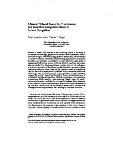
Figure 2.1: A one-layer Bayesian neural network with three binary input attributes and four classes. See the text for details.

where oii′ = 1 if xii′ ∈ A (i. e. if xii′ is among the observed evidence), and oii′ = 0 otherwise. Now we can compare this with the form in Eq. (2.7). In the neural network there is one input unit for each possible value xii′ of each input attribute Xi , and one output unit for each possible value yjj ′ of each output attribute Yj (typically one unit for each class, see Fig. 2.1). Then we can make the identifications βjj ′ = log P (yjj ′) wjj ′,ii′ = log

P (yjj ′, xii′ ) P (yjj ′)P (xii′ )

(2.11) !

sjj ′ = log πjj ′

(2.12) (2.13)

To make the activity of an output unit yjj ′ equal to the posterior probability of the corresponding class, an exponential transfer function should be used. However, since the independence assumption often is only approximately fulfilled, these equations give only an approximation of the probability. Therefore the formulas will eventually produce probability estimates larger than 1. To prevent this, one alternative is to use a threshold in the transfer function, which then looks ( 1 sjj ′ ≥ 0 πjj ′ = (2.14) exp sjj ′ otherwise Another alternative, which will be discussed more below, is to use normalization of the activities in the class units: exp sjj ′ (2.15) πjj ′ = P ′′ j ′′ exp sjj

To use a trained Bayesian neural network, the units corresponding to observed attributes are stimulated in such a way that their outputs, oii′, are set to 1. (All other oii′ are set to zero.) The activity is then spread through the weights Eq. (2.12) to the output units, which sum their inputs according to Eq. (2.7). This sum, or support value, of each unit is then fed to the transfer function Eq. (2.14), the result of which is returned as an estimation of the posterior probability of the corresponding class. For convenience, we will try to avoid the clumsy notation with double indices by suppressing one of them, when this can be done without confusion. Specifically, for the parameters in the ′ ′ network, rather than using ii and jj , the indices i and j will each range over all units in a layer, whenever it is not important to group the units into separate attributes. During training of the one-layer Bayesian neural network, the values of the weights and biases are determined by estimating the appropriate probabilities from the training data. There are at least two different approaches to this estimation, one stemming from classical statistics and the other from Bayesian statistics. We will take a closer look at them before going on with the training of the network.

2.2.1

Digression on Classical and Bayesian Estimation

The Bayesian neural network has its name from the use of Bayes theorem to calculate probabilities. There is nothing controversial with this. However, there is a slight controversy between two statistical schools:

16


the classical and the Bayesian school. The disagreement is to a large degree of a philosophical character. The classical school usually considers probabilities as an objective property of the nature, which can be measured with sufficient accuracy (and sufficient certainty) by repeating an experiment sufficiently many times. This is the frequentist interpretation of probabilities. The Bayesians on the other hand claim that probabilities merely signify our (lack of) knowledge of the world, and that they thus depend mainly on how much information we have about the situation [Cox, 1946]. This makes probabilities in one sense subjective, in that people with different knowledge assigns different probabilities to the same events [see also Jaynes, 1986]. As an example, consider a scientist whose assistant flips a coin, notes the result, and puts a handkerchief over it, without letting the scientist see the result. Clearly the scientist and the assistant have different opinions of the probability of the coin being heads up. In the same way, if we try to classify an insect from its appearance, it clearly belongs to some unique species, but we have to make an as good guess as possible from the known appearance. The more details we have observed of the insect, the more certain we may be of its species. Personally I believe that this philosophical difference is slightly overrated. First, it is quite common in real situations that the assigned probabilities differ between people just because they have different clues to go on (as in the above example), and this is not considered strange in any of the two schools. Second, there is nothing inherent in the Bayesian formalism itself which prevents a frequentist interpretation. Indeed, many of the examples to follow which describe the use of typical Bayesian formulas, are formulated in terms of ratios of large numbers of objects [see also Wolpert, 1994]. However, there are some differences in the way to approach a problem. The typical way to reason as a Bayesian, is that originally you have some, more or less vague, conception of the world. Then you make some observations or experiments, and given these you modify the conception to include the newly acquired knowledge. This can be repeated, so that further experiments may make your opinion of the world even more clear. In formulas this process is described as P (M | D) ∝ P (D | M )P (M )

(2.16)

where P (D | M ) is the probability of getting the data D given the current model M , P (M ) is the prior probability of the model, i. e. what you think about the world before the observations, and P (M | D) is the posterior probability, or what you believe after observation of the data (and ∝ denotes proportionality). The posterior probability can as mentioned be used as prior probability for a new set of observations (of the same process). Equation (2.16) is just another form of Bayes theorem where it is noted that P (D) does not depend on the model. It can thus be considered as a normalizing constant, which can be determined later by requiring that the posterior probabilities P (M | D) for all models should sum to 1. This brings us into another difference between classical and Bayesian statistics. Classically there is a difference between a probability distribution and its parameters. For example there may be a random variable X with a normal distribution with mean value µ and standard deviation σ. Then it is possible to talk about the probability of X having an outcome in some small interval, but it is normally not possible to talk about the probability of µ having some value. In Bayesian statistics the parameters are just another set of random variables with some distributions, corresponding to the uncertainty about their real values. If a number of samples are taken from the variable X, the parameter µ can (classically) be estimated as the mean value of these observations. But if this experiment is repeated, and the same number of samples are taken for each of several different estimates of µ, these estimates will differ slightly from each other. This motivates considering µ itself (at a fixed sample size) as a random variable. The interpretation is that after having seen a certain number of samples, there is a certain probability of the parameter having different values. Of course the standard deviation of µ gets smaller as the sample size increases, and the estimate gets closer to the “true” value. The classical way of estimating parameters in probability distributions is by Maximum Likelihood. This means that the estimated value of the parameter is the one that would have made the probability of the data as large as possible, i. e. which maximizes P (D | M ). The Bayesian way of thinking is rather that what ought to be maximized is not the probability of getting the data that we already got, but the probability of the parameter given the data, P (M | D). As can be seen from Eq. (2.16), the relation


17

between these two is just the prior probability distribution for the parameter, i. e. what we expect about the parameter (or about the whole model including its parameters) before observing the data. As an example, consider estimating the probability of heads on a (possibly unbalanced) coin by tossing it several times and counting the number of heads and tails. Let us call the parameter, the probability of heads, for p. The probability of getting cH heads out of c = cH + cT tosses is c P (D | M ) = P (cH | p) = (2.17) pcH (1 − p)cT cH To find the maximum likelihood estimate, differentiate with respect to p: d c c cH −1 cT P (cH | p) = cH p (1 − p) − cT pcH (1 − p)cT −1 dp cH cH c = (cH (1 − p) − cT p) pcH −1 (1 − p)cT −1 cH

(2.18)

Equating with zero (and ignoring the trivial solutions p = 0 and 1 − p = 0) gives cH · (1 − p) = cT · p cH cH = pˆ = cH + cT c

⇒ (2.19)

This is the classical estimate of the parameter p of a Bernoulli random variable. As expected, pˆ can be shown to converge to the “true” value of p when the number of tosses increases. However, for small sample sizes Eq. (2.19) may give unsatisfactory results. For example, if after three tosses there has been two heads and one tail, it gives that the most likely p is two thirds. However, if the coin were balanced, it could still not have been more even, so for such a small sample size it may be somewhat hasty to assume a pˆ so far from that of a balanced coin. Even worse, if after two tosses there has been two tails, Eq. (2.19) gives the estimate that pˆ = 0, i. e. that it is impossible to get a head. This is especially serious if the estimates are to be used as a basis for further probability calculations. Just because some event never occurred in the training data it does not necessarily mean that it is impossible. (Of course, we could test the estimate at some confidence level and reject it if it is too uncertain, but the point is that we do not want to reject any of the scarce data, but use it for exactly what it is worth.) Let us instead look at the Bayesian approach. Then we first need a prior distribution for p. Since the value of p may be anything, suppose first that we assume all probabilities p to be equally likely. Then the prior distribution of the model is P (M ) = P (p) = 1

(2.20)

(where P (p) is now actually a probability density function for p) and the posterior distribution becomes c P (M | D) = P (p | cH , cT ) ∝ (2.21) pcH (1 − p)cT cH Now, this is not a binomial distribution, since it is not to be considered as a distribution for cH any more, but as a distribution for the parameter p. Note that Eq. (2.21) is not an equality, but we have to normalize it to find the distribution. The calculation is slightly involved, but the result of integrating the right hand side (skipping the binomial coefficient which does not depend on p) is Z

1

pcH (1 − p)cT dp =

0

cH !cT ! (cH + cT + 1)!

(2.22)

This gives the distribution for p as P (p | cH , cT ) =

(cH + cT + 1)! cH p (1 − p)cT cH !cT !

(2.23)

18


which is a Beta distribution with parameters cT + 1 and cH + 1. Now, we are not really interested in the value of p which maximizes this (which would be the same p as in the classical case), but more in the expectation of p. To calculate E(p) we first use Eq. (2.22) again to evaluate the integral Z

1

cT

cH

p · p (1 − p) dp =

Z

1

pcH +1 (1 − p)cT dp =

0

0

(cH + 1)!cT ! (cH + cT + 2)!

and then use this to calculate the expectation Z pˆ = E(p) = p · P (p | cH , cT )dp Z (cH + cT + 1)! 1 = p · pcH (1 − p)cT dp cH !cT ! 0 (cH + cT + 1)! (cH + 1)!cT ! · = cH !cT ! (cH + cT + 2)! cH + 1 cH + 1 = = cH + cT + 2 c+2

(2.24)

(2.25)

This gives Laplace’s formula for successions. Note that for large samples this converges to the same result as the classical estimate, Eq. (2.19), but for small samples it will tend more towards the value 1/2. For example, for two tails in two tosses it still estimates the probability of a head in the next toss to 1/4. Also note that since we have arrived at a whole distribution for p we need not stop at calculating the expectation, but can also get the variance which can be used as a measure of how certain the estimate is. Usually the above prior for p is not used, but rather the more general form P (p) ∝ pα−1 (1 − p)α−1

(2.26)

for which a similar calculation gives the estimate of p as pˆ =

cH + α c + 2α

(2.27)

Note that this has as special cases the classical estimate when α = 0 and Laplace’s formula for successions when α = 1. The parameter α can a little sloppily be thought of as how much importance we give the prior and how much we trust the data directly. Equation (2.27) holds for a binary variable. A very similar derivation for a discrete variable with n different outcomes gives the estimate of the probability of the ith outcome: pî =

ci + α c + nα

(2.28)

In more detail, for an n-ary variable, the prior distribution for the parameters p = {p1 , p2 , . . . pn } is selected as P (p) =

n Y

pi α−1

(2.29)

i=1

This makes the posterior distribution of the parameters p a multi-Beta distribution: n Y Γ(c + nα) pi ci +α−1 P (p | c) = Qn · Γ(c + α) i i=1 i=1

(2.30)

Here Γ(x) is the gamma function which is defined for all positive real numbers and coincides with the factorial of x − 1 for all positive integers x. The normalizing constant is here determined only by identification with a multi-Beta distribution, and is not easy to calculate directly. Equation (2.28) is arrived at by, in the same way as in Eq. (2.25), identifying pi · P (p | c) with a new multi-Beta distribution, and take the quotient between the old and new normalizing constants.

19


The main critique from the classical statisticians is that a Bayesian needs to assert a “highly subjective” prior distribution before being able to calculate anything. However, in practice the Bayesian and classical results will converge very quickly to the same thing, as the number of observations increases, as long as the prior is “reasonable” (nonzero everywhere for example). Also, when so called non-informative priors are used, the results are in many cases identical to the classical results. The problem with the classical method of estimation is that it may not work well for small samples of data.

2.2.2

Training of the One-layer Network

The purpose of the training phase of the one-layer Bayesian neural network, is to determine the values of the weights wij and the biases βj . This is done by estimating the appropriate probabilities in Eqs. (2.11) and (2.12) from the training data. In the network there are counters for all units and all weights, to keep track on how many times each attribute value, and each pairwise combination of attribute values, has occurred. In detail, the counters are calculated as X C= κ(γ) (2.31) γ

cii′ =

X

(γ)

(2.32)

(γ) (γ)

(2.33)

κ(γ) ξii′

γ

cii′,jj ′ =

X

κ(γ) ξii′ ξjj ′

γ

(γ)

where γ is the pattern number in the training set, ξii′ indicates the presence of the attribute value xii′ in pattern x(γ) , and κ(γ) is the “strength” of the pattern. Typically κ(γ) is always 1, but it may take on other values if e. g. some patterns are more uncertain than others, or if a pattern represents several identical observations. (γ)

The values ξii′ need not always be binary (one if the ith attribute has value xii′ and zero otherwise), but can once again be probabilities, then interpreted as the proportion in the population described by pattern γ, having the attribute value xii′ . This is useful when describing the domain with prototype patterns rather than actual examples. If more than one attribute in a training pattern has graded probabilities associated to them, this is interpreted as if these probabilities are independent with respect to that pattern. This means that if two such “uncertain” attributes are not independent, then the pattern should be split up in two or more examples of the class, since one prototype is not sufficient to describe such a class. Training is done in one pass over the training set, during which the counters are updated for each sample, according to Eqs. (2.31) – (2.33). Thereafter the probabilities P (yj , xi ) and P (xi ) (and P (yj ), ′ ′ which is done exactly as P (xi )) are estimated from these counters. (Here the double indices ii and jj are replaced by single indices which range over the possible values of all attributes, to make the notation more simple). Let us begin with a classical estimation of the probabilities P (xi ) and P (yj , xi ). Classically the probability of an event is estimated as the number of observations where that event occurred divided by the total number of observations, that is ci C cij pîj = C pî =

(2.34) (2.35)

Since we are going to take the logarithm of these values, special care has to be taken when some of the counters come out as 0. In practice the logarithm of zero is replaced with a number more negative than all other values (of biases or weights) in the network. If we want the best probabilistic estimation of the distribution over the training samples, we should use a sufficiently large negative number to make sure that it outweighs all other contributions to a unit. But high accuracy of the distribution in the

20


training set does not guarantee good generalization. Even if a certain combination of attributes has never occurred in the training data, it may show up in a test pattern. If the maximum negative weight is too strong, this may then cause most probability estimations in the network to become zero. But we still want the least inconsistent alternative to get the highest probability. If sufficiently much speaks for a class, we want this to outweigh the fact that some attributes are contradictory according to the training set. Thus, the more negative a value is chosen instead of log(0), the better the accuracy of the probability estimates gets, but at the same time the generalization capability and fault tolerance in the network will decrease. Therefore a value just slightly more negative that the otherwise most negative value, for weights and biases respectively, are selected when a counter come out as zero [Holst and Lansner, 1993a]. The weights between units are set to  ci = 0 ∨ cj = 0  0 (2.36) wij = log 1/C cij = 0  log cij C otherwise ci cj

and the biases to ( log 1/C 2 βi = log ci /C

ci = 0 otherwise

(2.37)

The alternative way, which will also solve the problem with logarithms of zero in a natural way, is to use the Bayesian approach of section 2.2.1 to estimate the probabilities. Let the number of outcomes of Xi be ni and the number of outcomes of Xj be mj . Then the joint distribution P (Xi , Xj ) is considered as a distribution over a discrete variable with ni × mj outcomes. Now Eq. (2.28) can be used to estimate both pi and pij : ci + α/ni C +α cij + α/(ni mj ) pîj = C+α pî =

(2.38) (2.39)

Since these estimates are never exactly zero the calculation of weights and biases are straightforward: (cij + α/(ni mj ))(C + α) (ci + α/ni )(cj + α/mj ) ci + α/ni βi = log C +α

wij = log

(2.40) (2.41)

Note that the α used here is slightly different from that in Eq. (2.28). The advantage of using α in this way is that the marginal distribution of the prior is the same as the prior for the marginal distribution. The above weights and biases can be implemented in a straightforward way by initializing the counters C, ci and cij with α, α/ni and α/(ni mj ) respectively. The free parameter α is normally set to some small value. In the following tests the value α = 1/C is used. This gives the same order of the minimum bias value as in the classical case, i. e. ≈ log 1/C 2 . The Bayesian estimation of weights and biases was used throughout in the tests presented in this work.

2.3

The Independence Assumption

To derive the network model above, we had to assume independence between the different attributes, both unconditionally and conditionally given each class y, Eqs. (2.2) and (2.3). Complete independence in this way is of course usually not the case in real situations.

2.3 The Independence Assumption

21

Of the two relations the first one, Eq. (2.2), is actually less important than it might seem. To see this, note that Bayes theorem (2.1) can be written in the alternative form (which is the same as in Eq. (2.16)) P (y | x) =

P (y)P (x | y) P (y)P (x | y) =P ∝ P (y)P (x | y) P (x) y P (y)P (x | y)

(2.42)

Since the denominator is the same for all classes y, an error in it gives the same over- or under-estimation for all classes. This means that if we are only interested in the probability ordering of the classes, this is not affected at all. Furthermore, if we want the actual class probabilities we can always get them by normalization (since the probabilities P (y | x) must sum to 1 over all classes), thus compensating for this error. The second relation, Eq. (2.3), is more important since it directly affects the ordering of the classes, which of course is serious in a classification system. There is an important special case in which this relation holds though. It is when we can express each class with one single pattern, a prototype, and the instances are considered as noisy versions of this pattern. The prototype may have graded values of its attributes, representing the frequencies of different attribute values in the population. Some situations where this condition is likely to occur is when classifying an object (like an insect or plant) from some high level features of the object, where typically objects with similar feature vectors belong to the same class. Thus the independence assumption is related to the assumption that similar samples are likely to belong to the same class, where similar means that they have many attributes in common. If the same class can look in two entirely different ways (e. g. it is a mouse either if it has four small legs and gray fur, or if it has a button and a cord, but it will never have a combination of these appearances), it can not be described by only one prototype. Such cases may be less common in this kind of situation, but there are examples of domains where similar things can occur. For example, in medical diagnosis the existence of syndromes complicates the picture, since they consist of several symptoms appearing together. Also, the “one prototype” assumption is not appropriate for example in domains with strong invariances like character or speech recognition, or when trying to learn arbitrary logical relations. What we would like to do, to get as correct probabilities as possible, is to estimate the entire joint distribution over the whole input space X. This can of course be done by introducing “bins” for all combinations of outcomes and counting how many training samples that goes into each bin. When the number of training samples increases, the fraction of samples in each bin goes to the probability of that joint outcome. But if we have N binary events, 2N bins would be required (the curse of dimensionality, see section 1.1), and in practice we usually have a very limited amount of training data (and even if we had enough data, we would not have time to wait for the processing of it). This means that most bins will be empty, and we know very little about the distribution there. Instead we have to reduce the number of degrees of freedom in the problem. This will allow each training sample to give information about a larger part of the input space, which is necessary to achieve the desired generalization properties. To do this we must assume some additional structure of the problem, and if we do not know anything special about the domain, independence between events may be a natural choice [Chandrasekaran, 1971]. In spite of the possible violations of the independence assumption, the naive Bayesian classifier (and thus the one-layer Bayesian neural network) actually turns out to work surprisingly well in many situations, with results comparable to those of more advanced methods [Langley et al., 1992]. The gain in generalization from the events for which this assumption is correct, might to some degree outweigh the distortion in the probability from the cases where it does not hold within the domain. Important to remember is also that even if all units are not independent, the best we can do may be to assume independence, unless we know some extra structure of the problem, or have nearly unlimited amounts of training data. A more formal account for why the naive Bayesian classifier is often comparable to more advanced methods, can be found by considering the biases and variances of different classification methods [Geman et al., 1992; Friedman, 1996]. Still, in many cases there is some other structure of the problem which makes the independence assumption clearly useless, as in the parity problem, or when dealing with e. g. translation invariance or other invariances. Even in less extreme situations, this independence assumption is what limits the

22


operation of the one-layer Bayesian neural network the most. Therefore it is necessary to study some multi-layer extensions of the model that can help overcoming this limitation.

2.4

The Multi-layer Bayesian Neural Network

When all input attributes are not independent, the naive Bayesian classifier is not appropriate. If it were possible we would like to estimate the whole distribution P (X | Y ) directly, but this is impossible already for moderate numbers of input attributes. The solution we concentrate on here is to make something in between. Those attributes that are dependent must be considered together, but hopefully every attribute is not dependent on all others. In other words, we will try to utilize the independencies that can be found in the problem domain at hand. We will consider two different ways to handle dependencies [Holst and Lansner, 1996]. In the first, which is the simplest, the input attributes are partitioned into groups which are independent. Each group can be considered as one complex attribute, and the joint distribution over it is estimated. Since the different groups are independent of each other, their probability distributions can then be combined as before. The second method is more involved. It consists of trying to estimate a dependency graph between the input attributes, and uses this graph to calculate the joint probability distribution over the whole input space. If the domain had been continuous, and most distributions could be considered as mainly Gaussian, then some Principal Component Analysis (PCA) method [Joliffe, 1986] could have been used to generate a new set of input attributes (as linear combinations of the old attributes) which are approximately independent, and to which the naive Bayesian classifier could be applied [see e. g. Plumbley, 1993; Nadal and Parga, 1993]. However, when the domain is discrete (typically mainly with binary attributes) a PCA method is not so useful, since a linear change of axes will in general not make the new attributes independent in the sense we are interested in here. When we further on will treat continuous spaces, we will not make any assumptions of normality of the data, and thus we will not consider PCA in that case either. However, if the number of degrees of freedom in the domain is smaller than the number of input attributes, then some method (possibly PCA) could be used to select some subset of hopefully more independent attributes. There are several different methods for selecting relevant attributes [see e. g. Kittler, 1986; Battiti, 1994]. We will not consider them here either, but instead try to utilize all the information we get as well as possible. On the neural network side, the assumption of independence is closely related to the linear separability condition of the classes, which is required for one-layer networks (section 1.2.4). If the classes are not linearly separable, then the input attributes are not independent given each of the classes. (However, it does not hold the other way around; the classes may be linearly separable although the input attributes are not independent.) The normal way to solve this is to introduce a hidden layer in the neural network, and so we will do here. The hidden layer will consist of complex columns, groups of units which code for different combinations of activities of the same set of units in the input layer.

2.4.1

Partitioning Complex Columns

Suppose that two attributes Xi and Xj are dependent. Then we would like to consider their joint probability distribution P (Xi , Xj ) (and the conditional joint distribution P (Xi , Xj | y) for each class y), rather than the product of the marginal distributions. But if we manage to partition the input attributes into M independent groups (independent both unconditionally and conditionally given y), then we can introduce a “joint” variable Uk for each group. If the original variables Xi represent primary attributes, these new variables represent what can be called complex attributes. Now it is possible to express the distribution over the whole domain as a product

23

2.4 The Multi-layer Bayesian Neural Network

y1

y2

y3

y4

_

_

__

ab

ab

ab

ab

c

_

c

a

_ a

b

_ b

c

_ c

Figure 2.2: A multi-layer Bayesian neural network with a hidden layer consisting of one first order column C and one second order complex column AB.

involving the variables Uk , and instead of Eq. (2.4) we get M Y P (ui | y) P (x | y) P (y | x) = P (y) = P (y) P (x) P (ui ) i=1

(2.43)

The Bayesian model is now directly applicable on these complex attributes, via Eqs. (2.9) and (2.10). In the one-layer network each random variable is represented with one unit for each outcome of the variable. This means that the primary attribute Xi is represented with one unit for each value xii′. In the same way the complex attribute will now be represented with one unit for each combination of values of the original attributes it combines. This group of units for a variable Uk is called a complex column, and is placed in the hidden layer of the Bayesian neural network. Each unit in the column has connections from the units in the input layer it represents a combination of, and is active only when all its inputs are active. The structure of the network is now that a hidden layer with complex columns is inserted between the input units and the class units. Each complex unit has input connections from the input units it represents a combination of. Between these complex units and the class units is a layer of normal Bayesian weights, trained in the same way as in the one-layer case (see Fig. 2.2): P (ui | yj ) (2.44) wji = log P (ui ) One drawback with complex columns is that the number of units increases exponentially with their order, i. e. with how many input attributes they combine. However, it is not necessary to save the units for those combinations of values which never occur in the training data, since these will not contribute to the final classification. This can give a considerably lower number of units (unless the training samples have “graded” inputs). In the extreme case, when all input attributes are gathered in the same column, we will get one unit active for each training sample, i. e. grandmother units. (Also compare the architecture described by Protzel [1991], where the training samples are given one unit each in the network). Another problem with these complex columns is that when they grow larger, the generalization capability tends to decrease. This is the usual trade-off between probabilistic accuracy and generalization, and it should prompt us not to unnecessarily raise the order of the columns, but only introduce a high order column when it is actually required.

2.4.2

Overlapping Complex Columns

In many situations most attributes are slightly correlated with most other attributes. Even if only the strongest correlations are compensated for, the strategy of partitioning the attributes in independent groups may lead to unreasonably large columns. Suppose that the two attributes X1 and X2 are correlated, and so are X2 and X3 , but not X1 and X3 . Then we would have to join all three variables into a third order column, to compensate for these

24


dependencies. This should not be necessary, since there are only second order dependencies involved. (Actually, as the example is formulated there may well be a third order correlation between them, but let us assume for the moment that there is not.) It would be preferable if it was possible to create two columns, one for X1 and X2 , and one for X2 and X3 . But then these columns are certainly not independent, since they both contain the variable X2 . However, it is possible to adjust the formulas of the neural network so that this kind of “overlapping” columns can be used. Note that the important thing which makes estimation of the probability distribution over the whole domain possible, is that this distribution can be written as a product, only involving distributions of lower order. With the “order” of a vector random variable, or its (joint) probability distribution, is here meant the dimension of the vector random variable, i. e. the number of primary random variables that are combined. For a while we will ignore the classes, and concentrate on how to calculate the joint probability distribution over the input attributes, P (x). The method used here is similar to Chow and Liu’s tree dependency method [Chow and Liu, 1968], but also related to the methods used in Bayesian belief networks [Lauritzen and Spiegelhalter, 1988; Heckerman, 1995] (see section 1.2.3). Even if most input attributes in a domain depend somewhat on most others, it is likely that the domain is mainly governed by low order correlations. For example, in many domains it is meaningful to talk about the causal structure or dependency graph, a graph that describes how the attributes are causally connected [Chow, 1966; Chow and Liu, 1968; Pearl, 1988; Wedelin, 1993]. Even if all attributes are indirectly affected by most other attributes, the direct dependencies are usually of much lower order. If the dependency graph is a pure tree, then there is a simple method for combining lower order probabilities into a probability for the whole graph. Suppose there are three variables, A, B, and C. Now, if A affects B, and B affects C, then probably A and C are correlated too. However, if there is no direct connection between A and C not involving B, then it suffices to consider how B depends on A and then how C depends on B to calculate the joint probability distribution over all three variables. In detail, the joint probabilities can be written as P (a, b, c) = P (a)P (b | a)P (c | b) In general, all joint probabilities can be written as a product of conditional probabilities according to the chain rule: P (x) = P (x1 )P (x2 | x1 )P (x3 | x2 , x1 ) · · · P (xN | xN −1 , . . . x2 , x1 )

(2.45)

The last factor is conditioned on all the other attributes, so it still has the same order as the number of dimensions of the space. But if the direct dependencies form a pure tree (actually, it suffices that there are no directed cycles), the attributes can be sorted so that each of them only depends on variables it is conditioned on in Eq. (2.45). Also, each variable only has to be conditioned on the variables it has direct dependencies from, so all other conditioning can be removed from the factors in Eq. (2.45). This makes each factor have no higher order than the corresponding attribute’s number of direct dependencies plus one. If the set of variables which have direct dependencies to the variable Xi is denoted by Si , we get P (x) =

N Y

P (xi | Si ) =

i=1

N Y P (xi , Si ) i=1

P (Si )

(2.46)

Still assuming a tree dependency structure, note that the variables in each set Si must be independent. Each of them is the root of a dependency subtree, and since they all connect in the variable Xi , they can not connect anywhere else without causing a cycle in the dependency graph. Thus we can write the probability over Si as Y P (Si ) = P (xj ) (2.47) j:Xj ∈Si

With the help of this it is possible to rewrite Eq. (2.46) as an expression from which it is not clear in

25


d

d

b

f

b

c

f c

a

e

a

Figure 2.3: A directed dependency tree

e

Figure 2.4: A non-directed hypergraph

which direction the influence goes: P (x) =

=

N Y

P (xi ) ·

i=1

P (xi )

N Y

M Y

P (xi ) ·

i=1

P (x , S ) Q i i j:Xj ∈Si

P (xj )

Ψ(uk )

(2.48)

k=1

where to each nonempty set Si corresponds a new joint variable Uk combining Xi and all variables in Si , and Ψ(uk ) represents P (uk ) Xj ∈Uk P (xj )

Ψ(uk ) = Q

(2.49)

Each variable Uk takes care of a set of input attributes which are dependent, and it is not necessary to keep track of the causal direction of dependencies. This is an advantage, since it is not very well defined what is meant by causal connection between random variables. All there is statistically is correlation. As an example of how to rewrite the probability distribution over a directed dependency tree to an “undirected” expression, consider Fig. 2.3. First the attributes are sorted into the chain rule for probabilities: P (x) = P (a)P (b | a)P (c | ab)P (d | abc)P (e | abcd)P (f | abcde) Keep only the direct dependencies according to the graph: P (x) = P (a)P (b)P (c | ab)P (d)P (e | c)P (f | cd) Write the conditional probabilities as fractions: P (x) = P (a)P (b)

P (abc) P (ce) P (cdf ) P (d) P (ab) P (c) P (cd)

Finally, note the independencies between branches and rewrite: P (x) =P (a)P (b)P (c)P (d)P (e)P (f ) · P (ce) P (cdf ) P (abc) · P (a)P (b)P (c) P (c)P (e) P (c)P (d)P (f ) The result is of the form Eq. (2.48), i. e. containing all first order factors and then additional factors to compensate for the dependencies among these. This can be graphically represented in a hypergraph (a graph where each arc can connect more than two nodes) as in Fig. 2.4, where each arc represents a direct dependency of the same order as the number of nodes involved in it. Above we have assumed a pure tree structure. This implies that the arcs in the hypergraph meet at single nodes. We will not be that restricted though. It will be allowed with hyperarcs that have a common set of nodes, provided that there is a separate arc connecting exactly these common nodes.

26


y

y

1

ab

_

_

__

ab

ab

ab

a

y

y

_ a

b

2

a

_ a

3

b

4

_ b

_ b

c

c

_ c

_ c

Figure 2.5: A multi-layer Bayesian neural network with a hidden layer consisting of units for the input attributes, plus an overlapping complex column for a dependency between A and B.

This will give an opportunity to handle at least small cycles in an efficient way. Otherwise it will not be allowed with cycles in the hypergraph. The complete definition of the factors Ψ is then P (ui ) Uj ⊂Ui Ψ(uj )

Ψ(ui ) = Q

(2.50)

where the product is taken over all “sub-arcs” to the hyperarc Ui , and a sub-arc is required for every common set of nodes between two hyperarcs. Note that here the primary attributes Xi are included among the Ui (i. e. i ranges from 1 to N + M here), although they are not strictly considered as “arcs” in the graph. The interpretation of Eq. (2.50) is that for each direct dependency between a set of variables there is a factor Ψ(Uk ) which will adjust the probability by multiplying with the joint distribution and dividing by the “previous” product expansion for that distribution. Now, let us assume that we have the same causal structure on the attributes unconditionally as conditionally given y, which means that P (x) and P (x | y) can be expressed with the “same” factors, although for the latter they are conditioned by y: Y Ψ(ui ) (2.51) P (x) = i

P (x | y) =

Y

Ψ(ui | y)

(2.52)

i

The interpretation of the notation Ψ(ui | y) is that all probabilities in the equation for Ψ is conditioned on y. If Ui is actually a first order column Xi , then Ψ(ui ) = P (xi ) and Ψ(ui | y) = P (xi | y). We are now ready to write down the expression we want the network to calculate: P (x | y) P (x) Y Ψ(ui | y) = P (y) Ψ(ui ) i

P (y | x) = P (y)

(2.53) (2.54)

Taking the logarithm of this gives the same bias and support values as before, Eqs. (2.11) and (2.13), but a new expression for the weights from units in the complex layer: Ψ(ui | yj ) wji = log (2.55) Ψ(ui ) With this neural network architecture (see Fig. 2.5) the dependency graph is thus embedded in the hidden layer, and the probabilities are propagated through the neural network in one step. This is in contrast to Bayesian belief networks [Pearl, 1988], where the probabilities are sequentially propagated through the dependency graph itself.


2.4.3

27

Inhibition Between Columns

The definition of the factors Ψ, Eq. (2.50), is recursive. The Ψ for a random variable Ui consists of the probability distribution for that variable divided by the distributions of all “sub-variables” of it, i. e. all (possibly joint) variables that combine strict subsets of the variables that Ui combines. Sometimes the resulting recursive definition of the weights is inconvenient, or as we will see in the next chapter, not appropriate. Then the same calculation could instead be done with the help of “lateral inhibition” in the hidden layer. That is, instead of letting the weight compensate for already contributed effects from other columns, these other columns could be inhibited in the appropriate way. There is one tricky thing here. The inhibition should not simply inactivate another column. Rather it should subtract one unit of activity from the column. This means that if the column is inhibited from several other columns (because it combines a subset of the attributes of each of them), then it will actually get negative activity instead. Also, this inhibition has to be done recursively, in the sense that if a column is inhibited it has to remove the corresponding amount of inhibition from the columns it inhibits itself. Some work is thus moved from the training phase to the recall phase. When using inhibition in this way, the weights are again set to the original expression Eq. (2.44): P (ui | yj ) (2.44r) wji = log P (ui ) In each column (or alternatively in each unit) there is a counter keeping track of how many times that column is inhibited (in detail, its value is one minus the number of inhibitions). The output from the column (or unit) is multiplied with this counter before sent through the weights. When the network is passive all counters are zero. When a unit receives input from all input attributes it combines, it turns on and increases the counter by one. It also sends an inhibiting signal to all existing “sub-units”, units combining a subset of the attributes of the first unit. This makes these units in turn subtract one from their counters, but also recursively send to their sub-units to increase their counters by one. Since these later units are also sub-units to the original unit that got active, they will get both positive and negative signals. Dependent on the number of units “in between” the first unit and a sub-unit, the later may either decrease, increase, or leave unchanged its counter. Consider again the example of Fig. 2.3 and 2.4. It was found that the probability over the graph could be written as P (x) =P (a)P (b)P (c)P (d)P (e)P (f ) · P (ce) P (cdf ) P (abc) · P (a)P (b)P (c) P (c)P (e) P (c)P (d)P (f ) i. e. a product of the marginals, and additional factors for each hyperarc in the graph, to compensate for the dependencies. But it could also be rearranged to the form P (x) = P (a)0 P (b)0 P (c)−2 P (d)0 P (e)0 P (f )0 P (abc)P (ce)P (cdf ) = P (abc)P (ce)P (cdf )/P (c)2 In this example most first order factors get “inhibited” once by some higher order factor, and do thus not contribute at all, but note P (c) which gets “over-inhibited” and ends up twice in the denominator instead. This slightly complicated scheme is necessary to allow for unknown input attributes. This will be of great use later on, in Chapter 4. However, in domains where the whole pattern is given every time, the counters may be fixed once and for all when the dependency structure is determined. Because all columns will get exactly one unit active, the counter value for a column can then be determined by the total number of higher order columns containing the same attributes as the first column. When unknown attributes are used however, this number varies, since only the active columns are counted.

28


2.4.4

Digression on Iterative Probability Proportion Fitting

We have considered two different types of complex columns, partitioning columns, and overlapping columns forming dependency trees. These are both quite restricted in their form. It is an interesting question whether there are any more general methods to combine lower order probability distributions to higher ones. The problem is to estimate the joint probability P (X) given the marginal distributions of some (possibly different) orders. If we only know all the first order marginals P (X1 ), P (X2 ), . . . P (XN ) the “best” estimation (the least informative, and thus the best we can do if we know nothing more about the domain) is P (X) ≈ P (X1 ) · P (X2 ) · · · P (XN )

(2.56)

which is the usual equation for independent marginals. It seems intuitive that the more information we get about higher order marginals, the better should we be able to do on the joint distribution. As seen above, if the known higher order marginals form a dependency tree, then it is possible to adjust Eq. (2.56) with higher order factors. However, to get the best estimation given an arbitrary set of marginals is not equally easy. There is no closed form expression for the general case. It does not even help if we only consider the “simple” special cases when we know all second order marginals P (Xi , Xj ), or all marginals of some fixed higher order. However, there is an iterative method: the Iterative Probability Proportion Fitting (IPPF) algorithm [Brown, 1959]. This algorithm is so neat that it deserves a closer look. The task of the IPPF algorithm is to find the least informative joint probability distribution (the one with highest entropy) having a given set of (consistent) marginals. One property of this least informative solution is that it is also the expected probability distribution given the marginals, i. e. the average over all probability distributions whose marginals are equal to the given ones (when a uniform prior over the possible distributions is used). Here we will not give any proof that the IPPF algorithm really gives the least informative solution, nor that it is the expectation over all joint distributions, but only describe the algorithm. To illustrate the general principle, let us start out with a very simple example. Say that we have two (discrete) random variables X1 and X2 with known probability distributions. The algorithm starts by drawing a contingency table with, say, X1 to the left and X2 at the top, and initializing it with equal probabilities in each slot. The idea is then to iteratively scale the rows and columns to fit the respective marginals. That is, first the sum of each row is calculated, and the row divided with this sum and multiplied with the desired probability of that row, according to the marginal X1 . This makes the distribution in the contingency table have the correct marginal X1 . Thereafter the columns are scaled in the same way, i. e. dividing by the sums and multiplying with the desired marginal probability according to X2 . This may of course ruin the sum of the rows, but as these two steps are repeated, the probabilities in the table will converge to a distribution satisfying both marginals X1 and X2 . In the above example with two separate marginal distributions the probabilities will actually converge in only one turn of the algorithm, giving the trivial result that P (X) = P (X1 )P (X2 ). This is just what would be expected in this case according to Eq. (2.56). The real use of the algorithm is when there are a mix of higher order marginals, and no closed form expression for the joint distribution. For example, we may know P (X1 , X2 ), P (X1 , X3 ), and P (X2 , X3 ), and want to estimate the joint distribution P (X1 , X2 , X3 ) from this. Then the algorithm will use a “three-dimensional” contingency table, which will be scaled to fit each of the second order marginals in turn, until the contents of the table has converged. The IPPF algorithm can also be used when we have some apriori opinion about the joint distribution, and want to update this opinion in the light of new information about the marginals. Instead of initializing the table with equal probabilities, we just initialize it with our prior joint probability distribution, and then start to scale it according to the new marginals. The beauty of the algorithm is that it is so simple, and it will converge to the least informative solution whatever combination of marginals we know, as long as there is a consistent joint distribution.


29

The disadvantages is that it may sometimes converge slowly, and that for a high order distribution the contingency table may be too large to work with. Also note in this context that even if it is hard to find general methods to express probability distributions in terms of lower order distributions directly, one possibility is to express the joint probability as a product of potentials [Wedelin, 1993; Lewis II, 1961]: Y Q(Ui ) P (X) = i

Each potential depends only on a subset Ui of the variables in X. Typically the IPPF algorithm or some version of it can be used to find these potentials Q. We will not use the IPPF algorithm in the Bayesian neural network model, but try to stick to closed form approximations. The point here is that there is indeed a “best” solution to this kind of problem, and there is a simple iterative algorithm to find it, but that it does in general not exist a closed form expression which gives this solution.

2.4.5

Creating Complex Columns

If we can find the dependency structure, we can calculate P (x) with the help of this. The main idea is thus to first use the database to estimate the dependency structure of the domain. Then the database is used again to estimate the conditional probabilities of the classes, given that dependency structure. The problem of finding the dependency structure amounts to deciding which attributes to combine in complex columns, i. e. to find where the correlations are too high for the independence assumption to work. In general it is a very hard problem to find the independent partition of lowest order (possibly of exponential complexity, but compare the results of Blum and Rivest [1992] and Redding et al. [1991]). A partially heuristic method which has shown itself very useful though, is the obvious one of adding a complex unit to the hidden layer whenever some measure of correlation between two primary units is high [Lansner and Ekeberg, 1987]. This idea of incrementally creating higher and higher order units is quite common, and similar to a method described already by Ivakhnenko [1971]. In the context of columns this means that when the correlation between two entire columns is high, these columns are merged into one higher order column. “Merging” here means that a new column is created which considers the union of the input attributes of the two original columns as its input. The same method is used both for partitioning and overlapping complex columns, but with different restrictions on which columns are allowed. In the partitioning case two columns may not contain the same primary variable, whereas in the overlapping case the columns may not cause cycles in the hypergraph. Also, in the case of partitioning columns the two original columns are removed, whereas they remain in the case of overlapping columns. For this greedy heuristic method, the hidden layer initially consists of columns for all primary attributes, which can be considered as complex columns of order one. In the first pass, second order correlations are detected and removed by merging the corresponding attributes. Additional passes removes higher order correlations (i. e. pairwise correlations between higher order units) that has become visible by the previous passes. There are several different possible measures which can be used to quantify the “correlation” between attributes. What is wanted is not necessarily the traditional correlation coefficient, but rather a measure on how much the deviation from independence is expected to affects the results of the system. Depending on the exact purpose of the system, different measures may perform better than others [compare e. g. Levin, 1995; Kononenko, 1991c; Goodman et al., 1992; Redlich, 1993; Pazzani, 1995]. A number of measures has been evaluated in the Bayesian neural network for classification and diagnosis task [Holst and Lansner, 1992b, 1994], but that comparison will not be presented again here. The measure used in the following to check if a set of attributes are correlated, comes from information theory. The mutual information between two variables X and Y is defined as (see section 4.2 for further

30


details) I(X, Y ) =

X i,j

P (xi , yj ) log

P (xi , yj ) P (xi )P (yj )

(2.57)

If the mutual information between two attributes are above some threshold, they are considered dependent, and a complex column is created for them. All pairs of attributes are considered in this way, in order of decreasing mutual information. When used only one pass, this is the same method for generating a dependency tree as used by Chow and Liu [1968] (compare also with the method used by Cooper and Herskovits [1992]). However, here this process is continued a few passes, creating successively higher order columns compensating for higher order correlations. When partitioning columns are used, the mutual information between the higher order columns created in previous passes (or between complex columns and remaining primary columns) is considered. For overlapping columns a “generalization” of the mutual information has to be used: the Kullback-Leibler distance (also discussed in section 4.2) defined as X P1 (xi ) (2.58) P1 (xi ) log K(P1 , P2 ) = P2 (xi ) i where P1 (X) is the distribution acquired by merging the columns in question, and P2 (X) the approximation for the distribution before merging. When partitioning columns are used, or at the first pass of merging overlapping columns, P2 (X) will be just the product of the distributions over the columns to merge, and Eq. (2.58) degenerates to the mutual information Eq. (2.57). There are several reasons for using the mutual information (and Kullback-Leibler distance) instead of e. g. the correlation coefficient (besides giving the best result in the above mentioned comparisons) [see e. g. Li, 1990]. For binary variables, they give a pretty similar ordering, but for variables with more outcomes the correlation coefficient may be zero although the variables are indeed correlated. The mutual information is always greater than zero except when the variables are independent. Further, the mutual information generalizes nicely to the cases of more than two variables, and to overlapping columns (via the Kullback-Leibler distance). Also, the Kullback-Leibler distance can be interpreted as how “different” two probability distributions are (one being the distribution resulting from merging two columns, and the other the distribution if they are not merged), and may thus be a good measure on how much we gain by merging two columns [Lewis II, 1959]. Note that the method as described above will find the dependency graph in X, which is not necessarily the same as the dependencies in X | y. An advantage with this is that the method is unsupervised, which means that we can utilize unlabeled samples too. It also means that the whole training set is used for estimation of the same structure, rather than dividing it in separate groups for each class, which would give less confident values of the mutual information. If the causal structure is supposed to depend strongly upon the class, the conditional probabilities given the class can of course be used instead in Eq. (2.57), when deciding what columns to create. Although the chain rule works as long as there are no directed cycles in the dependency graph, and it is thus possible to write the joint probability over the graph in the form Eq. (2.48) even when there are some undirected cycles, we here only search for pure tree structures. This is because we never bother about the direction of causality, and thus can not distinguish between directed and undirected cycles. If the directions are known it is possible to treat undirected cycles too, with only a slight modification in how Ψ(ui ) is calculated. Also, small (directed or undirected) cycles can be handled by merging all variables in a cycle into one joint variable, or by triangulating the cycle. This is not treated further here however. After creating the hidden layer, the weights between the hidden units and the output units are determined in one pass by estimating the required joint probabilities P (ui ) and P (ui | yj ) from the training data and calculating the weights from them according to the above prescriptions.

31


a1 _ _

b1 b2 B

a2

a3

a4

_

ab11 pa1b1 pa2pb1 pa3pb1 pa4pb1 pa1pb2 pa2pb2 pa3pb2 pa4pb2

_

b3

ab pa1pb3 p 23 pa3pb3 pa4pb3 a2b3

b4

pa1pb4 pa2pb4 pa3pb4 pa4pb4

2.4.6

A

AB

Figure 2.6: A fragmented column AB with only two units, ab11 and ab23 . For all other cases the independence approximation P (ai bj ) ≈ P (ai )P (bj ) is sufficiently good, and we can thus use the activities in the columns A and B separately. If any of the units in the fragmented column goes active, it has to inhibit its corresponding units in A and B to ensure that we have activity in either A and B, or in AB only.

Fragmented Columns

The way complex columns are created according to section 2.4.5, is to merge two smaller complex columns whenever they are too correlated with each other. If the two columns are already quite big, we will get a very large number of new units, even if only a few of the original units were significantly correlated. As before this may impair the generalization in the network, when we have a limited amount of training data. In such situations it might be tempting to give up the column idea, and merge separate units instead of entire columns. It is nothing wrong in that as long as the resulting units get more uncorrelated, but this has to be done very carefully, not to introduce additional correlations instead. Fortunately there is no need to leave the column idea altogether. Suppose that we have two relatively large columns A and B, and suppose that the units inside them are mainly uncorrelated between the columns, such that P (ai bj ) ≈ P (ai )P (bj ). This means that we get good results even if the columns A and B are kept separated. But if now for one specific a ∈ A and one specific b ∈ B this is not fulfilled, a complex unit ab would be required to give a better result for this case. Thus there seems to be two distinct alternatives for the two columns A and B. Either we merge them to AB, and the result will be good for the case ab, but we will have a large number of units which requires more training data to estimate the densities reliably, or we let A and B be separated, and the results will be all right for the other cases ai bj but bad for ab. The solution is to use fragmented columns. Suppose that we in only the case ab use the corresponding unit from the column AB, and for all other cases use the units from A and B separately. Then we will get the good things from both alternatives (see Fig. 2.6). In general, if we have different alternatives of how to create complex columns, we can use fragments from each alternative if we make sure that only units from one alternative are active at one time. In the case of our example, it can be done by letting the unit ab inhibit unit a in A and unit b in B. This can be done with the same kind of inhibition that is discussed in section 2.4.3 above. Since now each column only contains a selected number of units, rather than units for all combinations of attribute values, it is not certain that each column has any active unit, even if there are no unknown inputs. This means that if this architecture is used, the inhibition counters can not be set beforehand, but has to be calculated dynamically during the recall phase in the network. One common situation in which fragmented columns are useful, is when dealing with letters in text. The inputs may be the letters in different positions in some string. If the string is from some natural language (rather than just a random sample of letters), there is certainly correlation between adjacent letters. However, to join two letter columns of 26 units each to one complex two-letter column would give 26 × 26 = 676 units. Since all two letter combinations probably consist of a relatively few which are much more common than if the letters were independent, and a large majority of them which are just slightly less common than if independent, it may suffice to create units for the combinations which are more common than “expected” from the independence assumption. (Some combinations perhaps never occur in practice, which then makes them much less likely than expected, but there is little point in making a unit for a combination which never

32


occurs.) If third order correlation (i. e. between three consecutive letters) are to be considered, the gain is even higher, and if the columns has to be even larger it becomes absolutely necessary to use the fragmented approach. The aim is then to create units representing possible “words” (or parts of words) in the string. For examples of such word detectors created with methods similar to the ones described here, see e. g. [Levin, 1995; Redlich, 1993]. Note that it is not necessary to save units in a column which have never been activated by the training data. They will have zero weights to all classes and will thus not affect anything. However, using the fragmented approach for those units may actually increase the generalization performance of the network. This is because the lower order columns can then be used for the combinations in a higher order column which have never occurred in the data. The effect of using fragmented columns is evaluated in section 2.5.4.

2.4.7

Class Conditional Structure

If the domain is really governed by some causal relationships, e. g. because it consist of separate components which interact through each other, then it is likely that the dependency structure is very similar for the unconditional case as conditionally given yj . However, just as there is no implication from the independence of two variables to the independence between them when conditioned on yj (nor the other way around), there is in general nothing that says that the best dependency tree when unconditional is the same as when conditioning on a specific class. Further, there is no guarantee that different classes should have the same optimal dependency tree. Since the important dependency is the class conditional one (the unconditional can be removed by normalization, see section 2.3) it may thus in general seem highly unmotivated to build the hidden layer based on the mutual information between the unconditional variables. When the domain is such that it can not be assumed to possess any global causal structure, it may be necessary with a slightly different scheme. The first simple idea is maybe to consider the mutual information in the class conditional distribution when determining which columns to create. This can of course be done, and should in these cases be more correct. The reason this was not always used here, is that the certainty in the probability estimations decreases rapidly when the data is split up in separate classes, and all probabilities are estimated separately from each. If there is a natural causal structure, it is better to try to detect this, since it gives more certain estimations, and it is likely to be nearly optimal for the class conditional distributions too. On the other hand, if there is no such structure, and we anyway have to estimate each class distribution separately, then there is an even more optimal solution. This is to use completely separate dependency trees for each class. This requires some small modifications to the current network. Note that in the calculation of P (x), we assumed X to have the same causal structure as each X | y. Now when the different class conditional densities are assumed to have different causal structures, they can certainly not all have the same structure as X. Thus we could not simply make the weights from a complex column to a class equal to the quotient (2.55) (which assumes the same arcs in the hypergraphs for the class conditional and the unconditional structure). Also, we could not use normalization of the classes after use of those weights with the previous argument that even if the calculation of P (x) gives the wrong result, it gives the same error to all classes, which would be canceled out by normalization. This is because the calculation of P (x) is no longer the same for the different classes, since they use different structures, so it will give individual error contributions to the different classes. The way to solve this is to remove the denominator from Eq. (2.55) altogether, to get the new expression for the weights wji = log (Ψ(ui | yj ))

(2.59)

and then use normalization over the classes. This gives the same error factor to all classes, i. e. the true value of P (x), so here the normalization will work.

2.5 The Technical Diagnosis Application

33

This is the strategy used by Chow and Liu [1968]. When there are sufficient training data and there is no reason to assume any global causal structure of the domain, this can be expected to give better results than using the unconditional version of the hidden layer. Both approaches to a class dependent complex column structure discussed in this section are evaluated in section 2.5.2.

2.5

The Technical Diagnosis Application

For evaluation of the Bayesian neural network with discrete input attributes a real world task has been used: diagnosis of faults in a telephone exchange computer. The task is to identify which of a number of circuit boards is malfunctioning when an error occurs in the APZ 212 processor of the AXE telephone exchange. The total number of circuit boards is 55, divided between two parallel processing sides, and a common coordinating part. When an error is detected (for example because the two parallel sides produce different results) the contents of several registers are dumped, giving an error vector of in total 1090 bits. This error vector is then to be used to identify the faulty circuit board, so that it can be replaced. The first study of a neural network on this task was done as a master’s thesis work by Gustafsson [1991], for Ellemtel Telecommunication Systems Laboratories. Since then the same database of errors has been used in several studies using different classification methods, which allows for a comparison between the Bayesian neural networks and the other methods. The database was constructed by inducing errors in a number of error points on (only) 36 of the 55 circuit boards. Not all of the 1090 error bits are present in the patterns though. This is because many of the registers contain pure memory addresses, and since only the board on which the error occurred is important, only the most significant bits from each address was used. Also, some registers were not considered relevant for the classification, and were thus removed completely [Gustafsson, 1991]. This left an error vector of 122 bits used for the classification of the 36 circuit boards considered. The database is split up in a training set of 442 errors and a test set of 112 errors. In the results below, there are four numbers quoted, labeled as “First”, “Second”, “Third” and “Other”. This is because most of the classification methods used give not only a single class as output, but a list of the most probable classes. In the case of the telephone exchange computer, if the error remains after replacing the circuit board most likely to be faulty, it is useful to have a few more alternatives to try to replace. Therefore not only the fraction of cases when the most probable suggestion is correct is shown, but also the fractions of cases where the second and third most probable suggestions are the correct ones.

2.5.1

Results with Various Methods

In Fig. 2.7 and Table 2.1 are shown the results of applying various methods other than the Bayesian neural networks to this task. These other methods are briefly described here. In connection with the telephone exchange computer there is a diagnostic program. This is what was used before the studies of neural networks for this task began, and it is in relation to this program the other methods should be viewed. These results were supplied by Ellemtel, together with the database. From the table can be seen that the diagnostic program manages to correctly classify about half of the cases. Since it is not trained from the database as the other methods, it is not as mysterious as it may seem that it is actually slightly better on the test set than on the training set. One very simple method for classification is the nearest neighbor classifier. This was used here, with the ordinary hamming distance (number of differing bits) as distance measure. This gives a good hint about the expected performance from methods which considers all input attributes as equally important. (Indeed, although not presented here, tests on the same database with a method based on Parzen estimators gave an almost identical result.) Such methods are clearly inappropriate in this case, since

34


Tested on training data

Tested on test data

100%

100%

80%

80%

60%

60%

40%

40%

20%

20%

0%

0% Diagnostic Program

Nearest Neighbor

One−layer Perceptron

Multi−layer Inductive Perceptron Tree (C4.5)

Diagnostic Program

Nearest Neighbor

One−layer Perceptron

Multi−layer Inductive Perceptron Tree (C4.5)

Figure 2.7: Classification results with the different methods. Black represents the fraction with correct first alternative, dark grey correct second alternative and light grey correct third alternative. See Table 2.1 for the exact numbers.

First Second Third Other

Diagnostic program 47.7% 7.2% 0.7% 44.3%

Tested on training data Nearest One-layer Multi-layer neighbor perceptron perceptron 95.0% 86.2% 90.5% 4.1% 1.6% 4.1% 0.7% 0.0% 0.7% 0.3% 12.2% 4.8%

Inductive tree (C4.5) 92.5% — — 7.5%


Diagnostic program 50.0% 5.3% 0.0% 44.6%

Nearest neighbor 42.9% 6.3% 0.9% 50.0%

Tested on test data One-layer Multi-layer perceptron perceptron 57.1% 69.6% 0.9% 8.0% 0.0% 4.5% 42.0% 17.9%

Inductive Tree (C4.5) 74.1% — — 25.9%

Table 2.1: Classification results with the different methods, tested on both the training and the test data sets. The percent of correct answers among the first, second and third best alternatives from the methods are shown, except for C4.5 which only gave a first alternative.

many of the input bits can be considered as mostly noise, whereas others are much more significant for the classification. Note that the classification result on the training data is not very relevant for this method. Since every input pattern has zero distance to itself, it would always be possible with 100% correct classification of the training set, unless as in this case the training set contains identical samples belonging to different classes. A third method used here is a one-layer perceptron. It had 122 input units and 36 output units, and was trained using the delta rule until convergence. It is included here mostly for comparison with the one-layer Bayesian neural network. The results of the multi-layer perceptron is taken directly from Gustafsson [1991]. The network used had one hidden layer of 30 units, and was trained using error back-propagation in 130 epochs. This was the configuration among several found to give the best results on this task. Both fewer and more training epochs were also tried, but that did not give any better results. Finally, the results with the inductive tree method C4.5 [Quinlan, 1993] is taken directly from a

35


Tested on training data

Tested on test data

100%

100%

80%

80%

60%

60%

40%

40%

20%

20%

0%

0% One−layer Bayes

Partitioning Overlapping Class−dep. Columns Columns Columns

Class−dep. Structure

One−layer Bayes

Partitioning Overlapping Class−dep. Columns Columns Columns

Class−dep. Structure

Figure 2.8: Classification results with the different Bayesian neural networks. Black represents the fraction with correct first alternative, dark grey correct second alternative and light grey correct third alternative. See Table 2.2 for the exact numbers.


One-layer Bayes 80.8% 12.2% 2.7% 4.3%

Tested on training data Partitioning Overlapping Class-dep. columns columns columns 84.8% 87.1% 89.6% 9.7% 7.2% 6.8% 3.4% 2.7% 1.1% 2.0% 2.9% 2.5%

Class-dep. structure 92.8% 4.8% 1.4% 1.1%


One-layer Bayes 61.6% 17.0% 5.4% 16.1%

Tested on test data Partitioning Overlapping Class-dep. columns columns columns 70.5% 75.9% 67.9% 13.4% 5.4% 10.7% 3.6% 6.2% 1.8% 12.5% 12.5% 19.6%

Class-dep. structure 60.7% 9.8% 8.0% 21.4%

Table 2.2: Classification results with the different Bayesian neural networks, tested on both the training and the test data sets. The percent of correct answers among the first, second and third alternatives from the networks are shown.

¨ master’s thesis by Ohman [1993]. This method did not give more than one class as output, so there are no numbers for second and third alternative correct. The best results on the test data are for the multi-layer perceptron and the inductive tree method. All methods except “nearest neighbor” outperformed the diagnostic program.

2.5.2

Results with the Bayesian Neural Networks

This section summarizes the classification results on the telephone exchange computer data with the different versions of the Bayesian neural network. In all cases each of the 122 binary input attributes and each of the 36 classes were coded with two units, one positive and one negative. Training of the weights and biases were done according to the Bayesian approach, Eqs. (2.41) and (2.40), with α = 1/C. The one-layer Bayesian neural network corresponds to the naive Bayesian classifier. Since it is a onelayer network it suffers from the same limitations of linear separability as e. g. the one-layer perceptron.

36


It is to this one-layer network the complex columns, either of partitioning or overlapping type, are added to get the multi-layer versions of the Bayesian neural network. The network using partitioning complex columns was acquired by merging columns in two passes, the first pass creating second order columns, and the second pass third and fourth order columns (by merging the columns from the previous pass with first order columns or with each other). The mutual information, Eq. (2.57), was used to evaluate each pair of columns for merging, and the threshold (the minimum mutual information required for merging) was set to 0.01. The resulting total number of columns in the hidden layer was 73, with in total 303 units (after units not used in the training set were removed). The network with overlapping complex columns was also acquired after two passes of column creation. However this gave at most third order columns, since only first order columns are considered for merging with an overlapping complex column. Note that unlike in the partitioning case the two previous columns are not removed in the process of merging them (see section 2.4.5). The mutual information Eq. (2.57) was used here too, again with the threshold 0.01. The total number of columns in the hidden layer was in this case 267 with a total number of 692 used hidden units. The three first bars and columns in Fig. 2.8 and Table 2.2 summarizes the results with these three Bayesian neural networks. The fraction of correct answers among the first, second, and third alternatives from the networks are shown. The results of all three Bayesian versions are comparable to those of both the multi-layer perceptron and the inductive tree. The two latter methods seems a little better when tested on the training data, but for generalization the advantage is more to the multi-layer Bayesian neural networks. If all the three first alternatives are considered together, the three Bayesian neural networks come better off on the training set as well as on the test set. The Bayesian neural network with overlapping complex columns gives the best result for generalization of all methods on this problem, and a result on the training data close to those of the multi-layer perceptron and the inductive tree method. (Note however that all these differences are quite small and may thus not be very significant.) The use of overlapping complex columns gives better results than using partitioning complex columns on both the training set and the test set. This can be explained by noting that Eq. (2.48) gives a better approximation to the distribution in the training set than Eq. (2.43), while at the same time using joint probabilities of lower order. The partitioning columns in this example are mainly of order four, whereas most of the overlapping columns are of order two and only a few of higher order. When creating complex columns in these multi-layer Bayesian networks, the correlations between input attributes were considered without regard to the class labels. This assumes a global dependency structure of the domain which is the same for all classes. In section 2.4.7 it was suggested that since the important thing is the class conditional dependencies, the class labels should perhaps be considered when creating complex columns. Two versions of class dependent complex columns were tried, both using overlapping complex columns. In the first, instead of using Eq. (2.57) directly when evaluating which columns to create, the expected mutual information over the classes was used. That is, the mutual information was evaluated for each class separately, and then weighted together with the class frequencies. This still gave the same dependency structure for all classes, but now compensating for the dependencies most relevant for the class distribution. These results are shown in the fourth bar and column in Fig. 2.8 and Table 2.2. In the second version a separate dependency structure was used for each class. Still Eq. (2.57) was used, but now for each class separately, using only the training samples from that class. The effect is the same as using different networks predicting the probability for the different classes. The results are in the fifth bar and column in the same figure and table as above. As can be seen, the results on the training data set is slightly better than with the original overlapping column version, whereas the results on the test data is clearly worse. The version with completely separate dependency structures has a larger tendency in this direction than the one using the same structure for all classes. The explanation for this is probably that the estimation of the mutual information within each

37


P Table 2.3: The total redundancy in the hidden layer, measured as R = i H(Xi ) − H(X), i. e. the sum of the information in the individual columns minus the total information they contain when considered together. The information here is measured in bits. The redundancy is shown versus the highest order of the columns used, for the two types of multi-layer Bayesian neural networks.

Partitioning columns Order Redundancy 1 18.6 2 11.5 9.4 4∗ 8 8.1 16 7.0 32 5.7

Overlapping columns Order Redundancy 1 18.6 2 8.2 7.6 3∗ 4 7.3 5 7.1 6 7.0 7 6.9 6.8 8

class is based on much fewer training samples, and thus much more uncertain than the estimation of the mutual information over all classes. The structure will thus be more sensitive to random fluctuations in the training data, and though this gives a better result on the training set, the generalization capability suffers. This effect is more severe when using separate structures for the classes, than when averaging the mutual informations for the different classes as when using the same structure. There is another important factor too. In this case it seems that it suffices to consider the global dependency structure when calculating the probabilities for the classes. This can be expected in e. g. technical domains, where the different input attributes correspond to parts in the system which are connected physically in some way. If on the other hand the dependency structure is considered merely as a means for approximating a probability density function (which is the main perspective here), and thus need not have any physical correspondence, then there is no reason to believe that the global dependency structure (as found when not considering the class labels during creation of complex columns) has any relation to the more important class conditional dependency structures. In those cases one of the two methods for incorporating class information during hidden layer construction may be used.

2.5.3

Redundancy in the Representation

One measure on how much of the correlations in the domain the complex columns manage to compensate for, is given by the redundancy in the representation in the hidden layer. The redundancy of a code is defined as the difference between the total information in the code, and the sum of the information in the individual parts of the code. If there is no redundancy, this difference is zero, whereas if several parts of the code contribute the same information, the sum is larger than the true information in the code. With partitioning columns the redundancy is straightforward to calculate in accordance with the above. When overlapping columns are used, some care has to be taken to get a useful measure. Since the original columns are not removed when a new overlapping column is created, the redundancy can only increase. However this is not what we are interested in here, since the idea with an overlapping column is that it should compensate for the effect of the lower order columns rather than replace it. Thus it should also compensate rather than add the information when calculating the redundancy. So the information contributed by an overlapping complex column is calculated as its “real” information minus the information contributed by the lower order columns combining strict subsets of the attributes of the first column. Table 2.3 shows the redundancy of the two different types of multi-layer Bayesian neural networks, for different numbers of complex column creating passes. Note that the highest order of the complex columns are doubled each pass when partitioning columns are used, but increased by one for overlapping columns. (This is because partitioning columns are compared to each other when searching for dependencies, but overlapping columns only to other first order columns.) The entries marked with a star correspond to

38


the versions of the multi-layer networks used in the comparison with other methods above. Order 1 corresponds to the one-layer network. The redundancy drops most rapidly during the first few passes of column creation, and then it levels off, for both network versions. In both versions the column construction is capable of reducing the redundancy considerably, but the overlapping columns manages to get the redundancy further down with lower order columns than when partitioning columns are used. (It is not certain that the redundancy can, or should, become zero, since the total information is calculated on the training set, and a redundancy of zero in the tables above would correspond to an extreme overtraining.)

2.5.4

The Effect of Fragmented Columns

The number of units in a column increases exponentially with its order, i. e. with the number of input attributes of that column. At the same time the generalization capability decreases, since there are usually too few training cases too cover all possible combinations of values of the input attributes for the column. When a unit in a complex column has never been activated during training, because that combination of attribute values never occurred in the training data, all weights from it will be zero. This means that the unit will not affect anything else in the network. However, it is possible that we could have done better if the input attributes had been considered independent in this case. Considering the supports from the individual attributes to the classes may give some hint about what the combination ought to support. This could at least give some clue about the classes if this combination of attributes should occur. As noted in section 2.4.6 on fragmented columns, it is not necessary to create units for all outcomes in an overlapping complex column. If there is a significant deviation from the independent case for only a few of the outcomes, only these have to be compensated for by the column. Specifically, if an outcome has never occurred in a column, there is no information at all about the correlation, and the best we can do is to assume that the corresponding input attributes are independent (or as dependent as indicated by possible lower order columns). Indeed, the results above for the multi-layer Bayesian neural network with overlapping columns were achieved when units for combinations which do not occur in the training data were never created. When partitioning columns are used, the effect of this is just a zero contribution from the column to the classes, if such a not represented combination of input attribute values would nevertheless occur in the test data. However, when overlapping columns are used, there is still a contribution from lower order columns (thus using the “independence assumption” when there is not enough data to estimate the joint probabilities). Here we will study more closely the effect on generalization and network size when fragmented columns are used. This is only applicable to overlapping complex columns, since with partitioning columns the lower order columns are removed. Table 2.4 shows the results of using varying thresholds for when to remove a unit from a complex column. The component of the mutual information contributed by each unit is divided by the order of the column (which in the case of only binary inputs is the logarithm of the number of possible units in the column, and thus compensates for the maximum possible value of the mutual information, which also increases as the logarithm of the number of units). If this is less than a threshold, the unit is removed from the column. Here the results of using thresholds 0.005, 0.01, and 0.02 are presented. For comparison, the results of saving all units, and of removing all units which are never used, are also shown. The latter is what was used in the results reported above for the Bayesian neural network with overlapping columns. For each different condition for removing units, the network was run through several passes of column creation, making columns of successively higher order. Order 1 corresponds to the one-layer network. No units were removed from the one-layer network, since units are only removed from higher order columns. As can be seen, a large saving of resources is made by removing units which do not occur in the training data. This is because the exponential growth of the complex columns with their order is stopped. For discrete attributes, there are never more units in a complex column than the number of training samples (and it may be much less, as in this case). Some further units may be removed by using a small threshold on the mutual information components from the units. Here a threshold of 0.01/order could be used

39


Order 1 2 3 4 5 6 7 8

None 244 584 776 1016 1368 1880 2776 3288

Number of hidden units Unused < 0.005 < 0.01 244 244 244 552 550 535 692 659 617 815 746 686 951 817 733 1084 888 783 1204 944 820 1254 959 834

< 0.02 244 478 529 569 597 626 646 653

Order 1 2 3 4 5 6 7 8

None 80.8% 86.9% 87.1% 86.9% 88.0% 87.8% 87.6% 88.2%

Tested on training data Unused < 0.005 < 0.01 80.8% 80.8% 80.8% 86.9% 86.9% 86.7% 87.1% 87.3% 86.9% 86.9% 87.1% 87.3% 88.0% 88.2% 88.0% 87.8% 88.0% 87.6% 87.6% 87.8% 87.6% 88.2% 88.2% 88.0%

< 0.02 80.8% 86.4% 87.3% 87.6% 86.4% 86.2% 86.4% 86.4%

Order 1 2 3 4 5 6 7 8

None 61.6% 75.0% 74.1% 74.1% 73.2% 72.3% 71.4% 72.3%

Tested on test data Unused < 0.005 < 0.01 61.6% 61.6% 61.6% 76.8% 76.8% 75.9% 75.9% 75.9% 74.1% 75.0% 75.0% 75.9% 75.0% 74.1% 75.9% 75.9% 75.0% 75.9% 75.9% 75.0% 75.9% 75.9% 75.0% 75.9%

< 0.02 61.6% 72.3% 70.5% 70.5% 68.8% 68.8% 69.6% 69.6%

Table 2.4: Results with fragmented overlapping columns. The topmost table shows the total number of units in the hidden layer for different passes of complex column creation and different conditions for removing a unit. The next two tables show the classification results on the training data and the test data. “Order” in all tables is the highest order of a column in the network, and corresponds to one plus the number of passes of complex column creation. The columns in the tables show the cases when no units are removed, when all unused units are removed, and when units which contributes less than 0.005/order, 0.01/order, or 0.02/order to the mutual information are removed.

40


53

109

54

110

55

111

56

112

57

113

58

114

59

115

60

116

61

117

62

118

63

119

64

120

65

121

53

109

54

110

55

111

56

112

57

113

58

114

59

115

60

116

61

117

62

118

63

119

64

120

65

121

93

75

86

94

80

81

82

83

100

101

102

7

103

104

105

9

47

48

49

44

45

46

24

25

26

27

80

81

82

83

100

101

102

7

103

104

105

9

47

48

49

44

45

46

25

26

27

89

73

90 87

72

91

71

92

15

36

16

35 31 17

34 19

30

33 38

85

98

84

97

28

41

29

42

85

98

84

97

28

41

29

42

37

93

75

86

94 89

73

90 87

72

91

71

92

15

36

16

35 31 17

34 19

30

33 38

24

37

Figure 2.9: The dependencies accounted for by the two versions of multi-layer Bayesian neural networks. The arcs in the first figure connect groups of units that are gathered together in partitioning complex columns in that network. The arcs in the second figure represent second order correlations between units, and correspond to the overlapping complex columns in the second network.

without reducing the performance. The reason for the decrease in generalization with higher order columns, when unused units are not removed, is hinted at above. The combination of attributes itself gives no information about the classes since it has never occurred in the training data. Instead considering the information from the different attributes separately (or from lower order combinations of the attributes) may at least give some crude hint about the classes, rather than no hint at all. In other words, when there is not sufficient data, considering the attributes as independent (or as having some lower order dependencies) may be the best we can do. The idea can be compared to the strategy used in many expert systems, of combining both general rules and specific rules dealing with exceptions to the general rules. The one-layer Bayesian neural network corresponds to an initial, possibly quite crude picture of the class distribution. The higher the order of a complex column, the more specialized features does it handle, thus making possible a more detailed picture. However, using fragmented columns allows the network to still use the “crude picture” for inputs for which the details are not known.

2.5.5

Analysis of Causal Structure

It was claimed in section 2.5.2 that the results were better with overlapping columns than with partitioning columns because overlapping columns are able to give a better approximation to the real distribution using columns of lower order than when using partitioning columns. It may be illustrative to look at the dependencies found and compensated for by the two versions. The upper part in Fig. 2.9 shows the causal structure compensated for when partitioning complex columns are used. The dots represent the different input attributes, and a line connecting two or more dots represents a complex column for those attributes. (The positions of the dots in the figure is chosen manually, and have no specific significance. Some attributes, not participating in any complex column,

2.6 Discussion and Conclusions

41

are not shown.) The lower part of Fig. 2.9 is the same thing for the network using overlapping columns. However, here each arc between two dots represent a second order correlation compensated for by one complex column. The third order columns are not shown, to avoid cluttering the figure. It is clear that for this database the overlapping complex columns compensate for many more dependencies than the partitioning complex columns. In the few cases where the former method does not compensate for a correlation that is found by the latter, this is because this would have created a cycle in the dependency graph. Some comments can be made about the structures found. The ladder-like structure to the left in Fig. 2.9 (in both dependency graphs) is due to two registers on each of the two parallel sides of the telephone exchange computer. They are supposed to have the same contents until something goes wrong, and are in general quite similar also when it does. This is a typical example of a strong correlation which is taken care of by the complex columns, to avoid these almost duplicate attributes to contribute the same information twice to the class units. To the right are four groups of units (100-101-102, 103-104-105, 47-48-49, and 44-45-46) which each turn out to be the three bits of an error code between one and seven. Such a binary encoded attribute is particularly unsuitable to use directly as input in a neural network (almost regardless of architecture), since all bits of the attribute has to be regarded together to mean anything. Both versions of the multilayer Bayesian neural networks have detected these groups (except the last group which is missed by the network with partitioning columns) and created third (or higher) order columns to deal with them. This has the effect of expanding these three bits into eight units, which is a much more suitable representation here. Note however that it is not at all certain that such binary encoded attributes are detected and expanded by the mechanism for constructing complex columns. To the contrary, such encodings can potentially give rise to parity type correlations, which are very hard to detect, and for which the independence assumption is particularly inappropriate. The reason they were detected here was that some error codes were much more common than others.

2.6

Discussion and Conclusions

In this chapter the one-layer Bayesian neural network, implementing a naive Bayesian classifier, was extended to a multi-layer network. This was done by introducing a hidden layer consisting of complex columns which compensates for dependencies between input attributes. Two different ways of using these complex columns were investigated. One way uses partitioning complex columns, which takes input from disjunct sets of input attributes. The objective of column construction is then to partition the input attributes into independent sets. In the other approach, overlapping complex columns are used. Each input attribute may then contribute to several complex columns (as long as there are no cycles in the hypergraph resulting from considering the complex columns as representing hyperarcs between the input attributes). This allows the same dependency structures as the ones used in Bayesian belief networks to be handled. Overlapping complex columns tend to give a better generalization performance than partitioning complex columns, since it is possible to get a better approximation to the real distribution using columns of lower order than when partitioning columns are used. To find an independent partition of lowest order of the input attributes (for the partitioning columns), or the dependency tree of lowest order (for overlapping complex columns) are hard problems, with no obvious algorithmic solution other than exhaustive search. This becomes intractable for domains with more than just a few input attributes. Therefore the complex columns are constructed using a “greedy algorithm” which searches for dependencies between already existing columns, and creates new columns to compensate for the found dependencies. This algorithm has shown itself efficient in reducing the redundancy (and thus in compensating for the dependencies) among the input attributes. The measure

42


used to determine how correlated two columns are, is the mutual information between the columns. This study has shown good results when applying Bayesian neural networks to diagnosis of a telephone exchange computer. The performance is comparable to that of e. g. a multi-layer perceptron neural network and an inductive tree method. The performance is similar for the three methods, but a tendency is that the Bayesian neural network is slightly better on generalization, especially when overlapping complex columns are used. Training of the Bayesian neural network is relatively fast (compared to the multi-layer perceptron), since this is done mainly in one pass, preceded by a few passes for construction of complex columns. Complicated technical systems which are hard to analyze, are good examples of domains in which neural networks can be useful. The Bayesian neural network proposed here is especially suited for use in these kinds of domains, since they often involve attributes connected in a causal structure. The possibility to depict the found dependency graph may also in itself provide a valuable tool in many domains.

Chapter 3

Graded Inputs and Continuous Valued Attributes In the previous chapter all input attributes were considered to be discrete, so that every outcome of every variable could be represented by one unit in the network. However, in many situations there are continuous valued attributes which give relevant information for the classification. In this chapter the model is extended to handle such continuous valued attributes as well. Before this it is however necessary to study a related extension. It was assumed that all input attributes were either completely known or completely unknown. A known input value would trigger the unit corresponding to that value to send its contribution to the classes. Sometimes the information about attributes may not be absolutely certain though. It would therefore be convenient if a probability distribution over an input attribute could be fed into the network. If there is some uncertainty about an input value this could be reflected in a graded input activity to the corresponding unit. One alternative could be to consider the attribute as completely unknown, but this would make the system loose useful information. Although they both concern graded values in some way, these two situations are very different in nature. The latter case concerns probabilities of discrete inputs (for example the probability that an animal has a tail), whereas in the former the inputs are themselves from some continuous domain (for example the length of the tail). In the Bayesian neural network model the activity of a unit is interpreted as a probability, so it is not appropriate to code a continuous attribute directly to an interval between zero and one and feed this into one unit. However, as will be seen below, the same mechanism that can handle arbitrary probabilities as inputs can be used indirectly to handle continuous valued attributes as well. This chapter first discusses how to treat graded inputs to the network, and how this can be used to handle uncertain evidence in the classification. Then continuous valued attributes are introduced, by using Mixture Models to code these attributes. Training of the mixture models is discussed, and a Bayesian version of the Expectation Maximization algorithm is presented. Finally the Bayesian neural network model with continuous valued attributes is evaluated on a set of real world classification problems.

3.1

Probability Distributions as Input

When deriving the key equations (2.9) and (2.10), it was assumed that we were given a set A of outcomes of some of the variables in the domain. For example we may be given that the variable Xi has the value xii′. Now we are instead interested in the situation when we are given the probabilities of the different possible values of Xi . In the case of a binary variable it of course suffices with one probability. With this new possibility the above mentioned equations have to be replaced.

43

44

CHAPTER 3. GRADED INPUTS AND CONTINUOUS ATTRIBUTES

Thus suppose we make a (non-conclusive) observation of an attribute, which leaves us with a distribution P (Xi ) over the corresponding variable Xi . Then we can express the probability of the class y given this distribution, using the probabilities of y given the individual outcomes xii′ of Xi , as X P (y | xii′) · P (xii′ | Xi ) (3.1) P (y | Xi ) = i′

The expression P (xii′ | Xi ) denotes the probability of the outcome xii′ according to the current distribution of Xi (and is thus not the same as the prior probability of the outcome). To condition on a whole distribution rather than on a specific outcome may seem unfamiliar at first, but is a standard approach in Bayesian statistics. To make clear what is meant by this conditioning, and to motivate more intuitively why Eq. (3.1) looks as it does, it may be suitable with an example. Suppose there are two car models, Volvo and Saab, and they both come in two colors, black and red. Say that both models are equally common, but they have different distribution of colors: 80% of the Volvos are black but only 40% of the Saabs. To find the probability of a car being a Volvo given that it is black, we thus take P (Volvo | Black) = P (Black | Volvo)P (Volvo) P (Black | Volvo)P (Volvo) + P (Black | Saab)P (Saab) 0.8 · 0.5 = = 0.4/0.6 = 2/3 0.8 · 0.5 + 0.4 · 0.5

=

Similarly, the probability of the car being a Volvo if it is red is P (Volvo | Red) = P (Red | Volvo)P (Volvo) P (Red | Volvo)P (Volvo) + P (Red | Saab)P (Saab) 0.2 · 0.5 = = 0.1/0.4 = 1/4 0.2 · 0.5 + 0.6 · 0.5 =

So, if we know either that a car is black or that it is red, we can calculate the probability of its model. Now, what if we only have acquired knowledge about the probabilities of the different colors ? Suppose that in a certain car park, into which we are not allowed to enter ourselves, the attendant tells us that there are currently 70% red cars parked. What is the probability of the first car leaving the car park being a Volvo ? We could expect that in 70% of the cases a red car leaves first. In those cases we know that the probability of it being a Volvo is 1/4. In the other 30% of the cases a black car comes first, in which we know that the probability of Volvo is 2/3. Thus we can just combine these numbers: P (Volvo | Attendants information) = =P (Volvo | Red)P (Red | Attendants info) + P (Volvo | Black)P (Black | Attendants info) =0.7 · 1/4 + 0.3 · 2/3 = 0.175 + 0.2 = 0.375 This last step is exactly the calculation prescribed by Eq. (3.1). In Eq. (3.1) the standard assumption is made that P (y | xii′) does not depend directly on Xi , i. e. that P (y | xii′) = P (y | xii′ , Xi )

(3.2)

This means, a little informally, that the car model should depend only on the real color, and not directly on how much we believe in that color. One could imagine cases in which this does not

45

3.1 Probability Distributions as Input

hold. For example, Volvos might be coated in some way which makes it much harder to see what color they actually have. Then the mere fact that we are uncertain about the color would be evidence in favor of the class Volvo. In most situations however, these subtleties will not have any real impact on the results. More importantly, in the context of continuous attributes, where this conditioning on probability distributions is used, this assumption is satisfied by other reasons. Note that the case when we know nothing about the ith attribute, is the same as when the distribution of Xi is the prior distribution. Conditioning on this unknown variable will in turn give the prior probabilities of the classes: X P (y | xii′) · P (xii′ | Xi ) P (y | Xi ) = i′

=

X

P (y | xii′) · P (xii′ ) = P (y)

(3.3)

′

i

When now trying to repeat the steps used to arrive at Eq. (2.10), there are some new considerations to make. The vector random variable X contains as before all the individual attributes Xi . But now we condition on the whole vector X rather than just the set A of determined attribute values. Unknown attributes have their prior distributions, other attributes the distributions resulting from the observation. We thus have that Y P (yjj ′ | Xi ) P (yjj ′ | X) = P (yjj ′ ) · P (yjj ′) i ! P Y ′ ′ ′ i′ P (yjj | xii ) · P (xii | Xi ) = P (yjj ′ ) · P (yjj ′) i   Y X P (yjj ′ , xii′)  ξii′ = P (yjj ′ ) · (3.4) ′ )P (x ′ ) P (y jj ii ′ i i

log P (yjj ′ | X) = log P (yjj ′ ) +

X i



 X P (yjj ′, xii′ ) log  ξ ′ P (yjj ′)P (xii′ ) ii ′

(3.5)

i

where ξii′ = P (xii′ | Xi ), i. e. the probability of a specific value xii′ of an attribute, according to the observation (i. e. the input pattern). Note that Eq. (3.5) contains the logarithm of a sum, which can in general not be simplified further. For completely determined input, i. e. when only one ξii′ is nonzero for every attribute Xi as in the previous chapter, this can be rewritten. Since then each sum consists of only one nonzero term is it possible to take the logarithm of each term separately, and then let some factors oii′ pick out which one to use. In detail, we can use that if the specific outcome xii∗ is the only outcome with nonzero probability, then it holds that   X X log  Wii′ξii′  = log (Wii∗ ) = log (Wii′oii′) (3.6) i′

i′

where oii′ = 1 if ξii′ = 1, and oii′ = 0 otherwise. (Wii′ could be any factors, but here represent the quotients in the inner sum in Eq. (3.5).) This gives the same result as in Eq. (2.10).

Also note that (incidentally) the same result, Eq. (2.10), holds when an attribute Xi is completely unknown, i. e. when according to the above every ξii′ has the apriori value P (xii′), since     X X P (yjj ′, xii′) P (xii′) log  Wii′ξii′  = log  P (yjj ′ )P (xii′ ) i′ i′   X = log  P (xii′ | yjj ′) = log 1 = 0 (3.7) i′

46


In the network the same result, i. e. 0, was achieved by setting all oii′ = 0 when Xi is completely unknown. Thus Eq. (3.5) reduces to Eq. (2.10) in the case when each input is either completely determined or completely unknown, in accordance with the claims in the previous chapter. However, when we now should anticipate arbitrary probability distributions as inputs, it is not possible to do this simplification. This does not give an as simple formula for the dynamics in the network as before. There are some different ways to handle this, a little dependent on the type of domain and how important it is that the network has a simple structure.

3.1.1

Use of the “Exact” Expression

The most natural approach, at least from the classification perspective, is perhaps to use Eq. (3.5) directly, as it stands. This will force us to use a slightly more complicated neural network structure than before. This is what has been used in the tests throughout this work. Overly more complex, the structure is not overly exotic for a neural network. Equation (3.4) has the same form as the combination function of a Pi-Sigma Neural Network [Ghosh and Shin, 1992], i. e. it contains a product of sums (rather than the more common case of sigma-pi units which sum a number of products). This type of network can be implemented by introducing an extra layer with units which do the inner sum (and take the logarithm of the result) and feed it to the original units doing the outer sum. This means that in this version the weights are most conveniently stored in the network “without” the logarithms: wii′,jj ′ =

P (yjj ′, xii′ ) P (yjj ′)P (xii′ )

(3.8)

Note that if the pi-sigma neural network architecture is used literally, the number of units required in the extra layer equals the number of input attributes times the number of output units (since each output unit has to sum the contributions to it from each input attribute, see Fig. 3.2). To avoid this large number of “purely administrative” units, the implementation used in the following does not have this extra layer. Instead the units keep track of which other units belong together in the same attributes, and sum within these groups before taking the logarithm and adding it all together. Logarithms are used instead of doing the product directly, because the numbers involved tend otherwise to become very large or very small before normalization.

3.1.2

Linear Approximation of the Logarithm

If the extra administration imposed by this double sum is considered a severe problem, there may, at least in some situations, be ways to get around this. One approach is to use Eq. (2.10) anyway, and claim that since it holds for the extreme values it will probably hold approximately in between too. This actually turns out to be a reasonable approach if there are only binary variables in the domain and if it is done in an appropriate way, but it may give too large deviations from the “true” values in the case of variables with more than two outcomes. Equation (2.10) holds when there is exactly one nonzero ξii′ for each attribute Xi , in which case the variables oii′ were used to pick it out. If we want to preserve the network structure with units that sum their inputs, the best we can do for other values of ξii′ is to choose oii′ to provide a piecewise linear approximation of the exact expression, Eq. (3.5). For a binary input attribute there are two input units in the network. Thus we want to approximate

47

3.1 Probability Distributions as Input

1

1

0.5

0.5

0 -0.5

0.2

0.4

0.6 ξi

-1

0.8

1

0 -0.5

0.2

0.4

0.6

0.8

1

ξi

-1

a

b

Figure 3.1: The desired support from one complementary pair of units on another unit, and some piecewise linear approximations of it. An example of the support from xi to yj according to equation (3.9) is shown as a dashed line in both figures. The parameters here are P (yj ) = 0.1, P (xi ) = 0.2, and P (yj , xi ) = 0.08. (a) The linear approximation that results if we set oi = ξi in (3.10). Note that this does not pass zero at the apriori value of ξi , 0.2. (b) The result of using (3.11), which gives a support that is both continuous and passes zero at the right place.

the desired support according to Eq. (3.5) from one such pair of units Xi = {xi , x¯i } on another unit y: ! X P (y, xi ) log ξi = P (y)P (xi ) xi ∈Xi P (y, xi ) P (y, x¯i ) = log ξi + ξ¯ P (y)P (xi ) P (y)P (x¯i ) i P (y, x¯i ) P (y, xi ) ξi + (1 − ξi ) (3.9) = log P (y)P (xi ) P (y)P (x¯i ) An example of what this function might look like is shown in Fig. 3.1 (dashed line). This will be approximated by an expression, linear in the activities oi and o¯i : P (y, xi ) P (y, x¯i ) log oi + log o¯i (3.10) P (y)P (xi ) P (y)P (x¯i ) If we let oi = ξi for continuous ξi , this yields a straight line between the values corresponding to strict binary input. This approximation is usually not very good (see Fig. 3.1a). If y is positively correlated with xi , then it is negatively correlated with x¯i . This means that the logarithm changes sign somewhere between the end points. This change of sign occurs exactly when we do not know anything about xi , and thus ξi = pi (where pi is used to denote the estimated prior probability P (xi ) of the unit). When we do not know anything about xi , its pair of units should not influence anything else in the network, i. e. its output should be zero. But the linear approximation above does generally not pass zero at that same point. Since we have two units it is actually possible to instead approximate the influence with two linear pieces, by e. g. letting unit i be active only for ξi above the prior probability pi , and unit ¯i active below pi . By letting both oi and o¯i be zero when ξi = pi , and increase linearly from that point in their respective directions, the result will coincide with the desired support in the same three points as before (“yes”, “no”, and “unknown”) and be a linear approximation in between these points (Fig. 3.1b). Expressed as a function of ξi , oi becomes ( 0 ξi ≤ pi oi = ξi −pi (3.11) pi < ξi 1−pi The last approximation is based on the requirement that the function fits exactly in the extreme points, and when crossing zero. The assumption is that most attributes are either unknown or completely determined, and thus this gives as few as possible contributions deviating from the “true” values. If for

48


Class units

Π

τ

Class units

Σ

Complex units

Complex units

Input units

Input units

Figure 3.2: A Bayesian pi-sigma neural network, which implements (2.9) directly. Each class unit has one unit for each complex column, summing up the contribution from the whole column.

Figure 3.3: A Bayesian neural network with spiking units and an extra layer of time averaging units at the outputs.

example a minimum square distance approximation method had been used, quite another approximation would have resulted, but this would have been optimal only if all input probabilities were equally common. There is no immediate reason why oi can not be a non-linear function of ξi . One could imagine any non-linear relationship, for example one that gives exactly the wanted curve Eq. (3.9). The problem is that this would be adapted only to a specific class y, and the same activities oi is to be used for all classes. The only thing which is the same for all classes is the point where Eq. (3.9) crosses zero. The values for ξi = 0 and ξi = 1 are also different for all classes, and is not constrained by where the zero crossing is. This difference is contained in the two weights from the two units to a specific class unit. The only thing which remains for oi to determine is to what degree all the outgoing weights should be used. Since not even the first derivative of Eq. (3.9) at the zero crossing is the same for all classes, it is very hard to do better than a linear approximation. The main problem with this linear approximation is for conditional probabilities close to zero, i. e. when the probability for a class given an attribute value is very small. In that case the logarithm will be a large negative number, and Eq. (3.9) is very steep close to this end. This can cause a very large difference between the linear approximation and the real curve. Also, for more than two possible values of an attribute Xi it is hard to find a good approximation. A generalization of the above to the case of n non-negative ξii′ summing to 1.0, and which yields a piecewise linear approximation of the logarithm that is exact in the n extremal points and in the “unknown” case, requires a kind of normalization of activities in each group: ki = min ξii′/pii′ ′

(3.12)

oii′ = ξii′ − ki pii′

(3.13)

i

This will however already for small n in the general case fail to come close to the real logarithm for most other inputs than the extremal ones. Thus this approach is clearly unsuitable when the domain is not confined to binary attributes, and specifically when there are continuous valued attributes.

3.1.3

Implementation with “Stochastic Spiking Units”

Another variant is to use stochastic spiking units. In more detail, each unit has in a specific moment either activity 0 or 1, but shifts between these values such that the probability of having activity 1 at any moment represents the probability of the corresponding feature [Lansner and Holst, 1996]. By always having binary inputs, Eq. (2.10) will always hold. However, now the average over time of the activity in an output unit reflects the posterior probability of the corresponding event. To achieve the correct outputs, the activities of the output units is thus averaged over a sufficiently long time (with the same input pattern).

49

3.2 Uncertain Evidence

Note that this reflects in some sense a natural interpretation of graded input and probabilities here; it corresponds to the proportion in a large number of cases that a certain feature is expected to occur. The term “spiking” in this context comes from the view of having biological spiking neurons, each with a probability of giving a spike in a certain time slot. Of course, the “probability” corresponding to a neuron spiking with a certain frequency depends on the length of the time slots, so this length should be selected in relation to the maximum spiking frequency of the neuron, for the probability interpretation of activity to lead over to the biological case. Consider again the probability of a class y given the probability distribution of Xi . It can be written as the expectation of the probability over all outcomes xii′ of Xi : X P (y | Xi ) = P (y | xii′) · P (xii′ | Xi ) = EXi (P (y | xi )) (3.14) i′

If we can generate a series of xi with the distribution Xi and average P (y | xi ) over them, we will get a result that converges to the expectation in Eq. (3.14), and thus to the probability P (y | Xi ). For this to work, the correlation in spikes between two units must be the same as the correlation between the corresponding attributes. Since input attributes in this model are not necessarily independent, and it is hard to generate appropriately correlated spikes (note that we do not have access to the joint distribution over the domain, since this is what we are trying to approximate), this may be a problem. When partitioning complex columns are used, the spiking units are therefore introduced in the hidden layer of the network. These complex columns are supposed to be independent, so units in different complex columns can generate spikes independent of each other. It is important though that only (and exactly) one unit is active at a time in each complex column. Together with overlapping complex columns it is more complicated, since the spikes generated in different columns with some attributes in common must always match each other (i. e. the values of the common attributes must be the same due to the spikes in all columns at each time slot). There is no obvious way to generate such spikes. With overlapping columns it may therefore be necessary to generate the spikes at the input layer anyway. The stochastic activities in the hidden layer are fed through the Bayesian weights to the class units, and running averages of the unit outputs are calculated. This can e. g. be done with an extra layer of “leaky integrator” units (see figure 3.3). The computational structure in this network is considerably less complicated than that of the pi-sigma network (figure 3.2). This may also make this approach more suitable for hardware implementation.

3.2

Uncertain Evidence

One important purpose of the above treatment of graded input is to be able to handle continuous valued attributes. How this is done is shown in the next section. However, if the network is to be able to handle uncertain evidence from the user, then there are some further details which need to be addressed. If there are no complex columns in the network, the introduction of uncertain evidence is quite straightforward. The probability distribution of each attribute after an observation can be fed directly into Eq. (3.5) (as the values ξii′). One objection is than in a typical situation the value of uncertainty from the observation is not the same uncertainty one is supposed to feed into the network. The network expects the probability of the feature in question given the possibly non-conclusive observation of it. But if a measurement is done with some partially unreliable instrument, what is known is instead typically the probability of error for the instrument, which means the probabilities of the instrument showing certain results given the real feature. What has to be done is, once again, to “invert” the conditioning via Bayes theorem, Eq. (2.42): P (feature | observation) ∝ P (observation | feature) · P (feature)

(3.15)

A more severe problem is perhaps how to use graded inputs in connection with complex columns. For completely determined input values of some primary attributes, the activity of a complex unit can be

50


calculated by multiplying the activities of the units it represents a combination of. This would also be a good idea in the case of graded input, if the primary attributes were independent. But the very reason to create the column for a set of attributes is just that they are not independent. With at least one specific model of the uncertainty in the observations, this problem has a simple solution. Assume that two features, f1 and f2 , (which are dependent) are measured with two measuring devices, giving the results e1 and e2 . Suppose now that the probability of error in each of the measuring devices are independent of each other, i. e. an uncertainty in one measurement does only depend on the feature it was supposed to measure, and not on the other feature (this is not an unreasonable assumption). Then what is known is the probabilities P (e1 | f1 ) and P (e2 | f2 ). But since these observations are not directly dependent on other features than the ones they try to measure, we can write P (f1 , f2 | e1 , e2 ) ∝ P (e1 , e2 | f1 , f2 )P (f1 , f2 ) = P (e1 | f1 )P (e2 | f2 )P (f1 , f2 )

(3.16)

So if the user tells the system the probabilities of making the current observations given the possible values of the attributes, then the system can combine this information and feed it into the hidden layer of the network, just using multiplication and normalization. In the general case, when there is no specific model of the noise, or the uncertainty, the problem is harder. The trouble lies actually already in the problem formulation. We would like to calculate the distribution of AB from the marginal distributions A and B. But if two attributes are not independent, it is not sufficient to know their marginal distributions, to be able to calculate their joint distribution. One the one hand, this would require the user to specify the joint distributions for every complex column in the network. On the other hand, the exact complex column structure in the network is normally not accessible to the user (normally the user do not want to bother about the internal structure of the network). Further, if the probability distribution over an attribute given an observation is hard to specify for the user, then the joint probability of two or more attributes is worse. However, there is actually a general way to find a joint distribution when the user has only supplied the marginals. The situation is similar to the one discussed in section 2.4.4, where the task was to find the expected joint distribution given a set of marginals of different orders. The difference here is that now the prior joint distribution is known (which among other things contains information about “how correlated” the marginals are). The IPPF algorithm from section 2.4.4 can be used in this case too. The prior distribution is fed in as initial data in the contingency table, and the algorithm runs as usual from there, producing the expected posterior distribution. (For just a pair of binary variables, the expected joint distribution can also be found as the solution of a quadratic equation, but for the general case with a higher number of marginals, there is no exact closed form solution.) To illustrate that this is a question which actually has a unique answer, consider again the car park example. Still there are equal numbers of Saabs and Volvos in the world, and 80% of the Volvos and 40% of the Saabs are black, and the rest red. Suppose now that the car park attendant tells us that there are currently 70% red cars, and 60% Volvos parked inside. What is the probability that the first car leaving the car park is a red Volvo ? Thus, we know the prior distribution of car models and colors in the world, but in this specific car park we know the proportion of Volvos and the proportion of red cars separately, and we want to find out the proportion of red Volvos. Consider all possible ways to put Saabs and Volvos in the car park. Now pick out only those ways which contain exactly 70% red cars and 60% Volvos. The proportion of red Volvos among all those cases is the objective answer we are looking for. In the case of only two attributes (model and color) it is possible to set up an expression for this and solve it. It will in this case give the result that there is about 34.4% chance of a red Volvo. The IPPF method gives the same answer and is much more straightforward to use. We will not bother with either calculation here however. The point is that this is a well defined question with a well defined answer. Note that in contrast to the trouble of propagating graded input activities from the primary attributes to a complex column, the other way is somewhat easier. To calculate the probability of an outcome of a

51

3.3 Continuous Valued Attributes

primary attribute, it is just to sum over the units in the complex column which belong to that outcome. This is useful for partitioning complex columns. If overlapping columns are used, there is already one column representing each primary attribute which can be used directly. The conclusion is that if uncertain evidence is to be treated, one of the above mentioned methods for this should be used. One could on the other hand argue that if the uncertain inputs stem from subjective user judgments, they may themselves not be so accurate as to require any too advanced treatment. Some approximation which just makes the input probability be above the apriori value when the user judges it to be more likely than normally, and the reverse when it is judged as less likely, may well be sufficient in many situations. Here we will not treat uncertain evidence and graded user input further, but concentrate on the continuous valued attributes instead.

3.3

Continuous Valued Attributes

In the above we have assumed all attributes to be binary or discrete. When graded input occurs, it is as probabilities over the attributes. Here we will handle the situation when the evidence we want the network to use comes from a measurement with a result in some continuous interval. It is not possible to code the continuous attribute directly as graded input activity of one unit in the network, since this would then be interpreted as a probability. For example, the result of giving a fifty percent probability for a binary feature will always be an equal mix of the situations when the feature is present and not, whereas a medium sized object does not necessarily have properties exactly between those of a large and a small object. The same mechanism that allows uncertain inputs in the Bayesian neural network model, can however be used indirectly to handle continuous valued attributes. The idea is to transform the continuous variable into a number of discrete variables, which can be used directly by the Bayesian network. This is done via a Mixture Model [McLachlan and Basford, 1988; Tr˚ avén, 1993]. The probability density function over some continuous variable Z can be approximated by a finite sum (although it is a density function, it is here denoted by P (z)): P (z) =

n X

P (vi )P (z | vi )

(3.17)

i=1

This can be seen as a partition of P (z) into n sub-distributions P (z | vi ), each with probability P (vi ) of being the “source” of z. Expressed in another way, random numbers with the distribution P (z) can be generated by first selecting among the sub-distributions with probabilities P (vi ), and thereafter generating the number from the selected distribution P (z | vi ). The above equation also defines P (vi | z), the probability of each component vi being the source of a given z, as P (vi | z) =

P (z | vi )P (vi ) ∝ P (z | vi )P (vi ) P (z)

(3.18)

where instead of keeping track of P (z), we can again use normalization (over i) of the right hand side. Suppose that we are interested in the distribution of weights among the various animals in our garden. We place a weighing machine in the garden and every time an animal happens to step onto it, the weight is registered. There are cats, rabbits, and squirrels in the garden, in different proportions. Say that the weights within each species is approximately normally distributed, but with different means (and variances) for each species. Then the total distribution will be a weighted sum of these three normal distributions: P (weight) =P (weight | cat)P (cat) + P (weight | rabbit)P (rabbit) + P (weight | squirrel)P (squirrel)

52


In this example the distribution consist of three “true” sub-distributions, and it is natural to talk about the probability of the weight being generated by “a cat” or “a squirrel”. However, in general a mixture model can be used to approximate a distribution, regardless of whether there is any real underlying subdivision in different “sources”. Typically the component densities are selected to be localized functions, in the sense that they have each one peak and decrease monotonically with the distance from this peak. They should preferably decrease sufficiently fast to be in practice negligible outside some reasonable radius. This is the case assumed here, but the equations below hold for other choices of component functions too. It is common to use Gaussian functions as component densities, and thus to talk about Gaussian Mixtures. At least in the case of a one-dimensional variable Z such a localized mixture model can be thought of as giving rise to a kind of soft interval coding. Each value in the interval will “belong” to different degrees to the different components, which thus makes a soft division of the interval between themselves. Of course an analogy of this holds also in the multi-dimensional case, where each component dominates some local piece of the input space. This is reminiscent of the coding used in the context of fuzzy sets [Zadeh, 1965], although the interpretation of activities is here in terms of probabilities rather than of fuzzy memberships. Note also that the use of soft interval coding to represent continuous input attributes is abundant in biological nervous systems. Some examples include: orientation selectivity of simple cells in visual cortex [Daugman, 1989], the tuning curves of auditory cells, response properties of vestibular hair cells [Kandel et al., 1991], wind detection cells in crickets [Salinas and Abbott, 1994], etc. Even motor output is to some degree organized along the same principles, taking advantage of recruitment and population coding [Fuglevand et al., 1993; Georgopoulos and Lukashin, 1994]. If the component functions are chosen “close enough”, we may assume that this coding preserves the information in the original value of z, i. e. that a class y depends only on z via the values of vi : P (y | vi , z) = P (y | vi )

(3.19)

This also implies that z only depends on y via vi : P (z, vi ) P (y | vi , z) P (y, vi ) P (z, vi ) P (y | vi ) = P (z | vi ) = P (y, vi )

P (z | vi , y) =

(3.20)

This assumption is very natural if the mixture components represent some “real” partition of the inputs into different categories. Then the class usually depends only on which category some object belongs to, and the input value is used only to find the probabilities of the different categories (as in the animal weight example, where the categories represented by the mixture components were the same as the animal classes). If the mixture components are selected merely to approximate the real distribution, and not because they are a natural categorization, some care should be taken to assure that the components are really close enough not to distort the classification too much. Using Eq. (3.19) we come to the key relation in this context, i. e. how to calculate the probability of a class given z using a set of suitably selected component functions P (vi | z): X P (y | vi , z)P (vi | z) P (y | z) = i

=

X

P (y | vi )P (vi | z)

i

= P (y)

X P (y, vi ) P (vi | z) P (y)P (vi ) i

(3.21)

53


This is easily generalized to the case of a set of independent continuous variables zi : Y P (y | zi ) P (y) i Y X P (y, v ′) ii = P (y) P (vii′ | zi ) P (y)P (v ii′) ′ i

P (y | z) = P (y)

(3.22)

i

Just as in the other cases above, what is treated by the network is the logarithm of this probability:   X P (y, v ′) X ii log  log(P (y | z)) = log(P (y)) + P (vii′ | zi ) (3.23) P (y)P (v ii′ ) ′ i i

This is analogous to Eq. (3.5), where the input probabilities ξii′ = P (xii′ | Xi ) in the case of graded input, are replaced by the probabilities that a continuous input value “belongs” to the different component distributions of the mixture model, P (vii′ | zi ). (The assumption that the classes depend on the distribution of an attribute only via the actual attribute value, Eq. (3.2), is here replaced by Eq. (3.19).) With the help of a mixture model it is not only possible to calculate the probabilities of the classes or other discrete attributes, given the continuous variable. It is also possible to use the network for prediction of a continuous value, given some other attributes. The first step is to retrieve a continuous value from the probabilities of the different component functions, P (vii′ | x) (where x represents some presented pattern which does not include zi ). Since this representation is in terms of a whole distribution, and we want a single value out, it may be reasonable to use the expectation of zi , E(zi ) =

n X

E(zi | vii′)P (vii′ | x) =

i′=1

n X

µii′P (vii′ | x)

(3.24)

i′=1

where µii′ is the expectation of the component function P (zi | vii′) (or its mean value). If the component function is symmetric with a single peak, this µii′ will be exactly at the peak. Now we can calculate the expectation of another continuous variable yj given zi . Let yj have the component functions P (yj | ujj ′) with expectation (or peak at) ηjj ′, and we have analogously to (3.21) E(yj | zi ) =

X j

=

X j

ηjj ′ P (ujj ′ | zi )

′

′

 X P (ujj ′ , vii′) P (vii′ | zi ) ηjj ′ P (ujj ′) P (ujj ′)P (vii′ ) ′ 

(3.25)

i

Of course this also generalizes to the case of a set of independent variables Z. Thus when using the network, the values of known continuous variables are first propagated to a layer of units the activities of which represent the values P (vii′ | zi ). This layer is fully connected via Bayesian weights to the output layer, with units representing the sub-distributions ujj ′ of continuous output variables Yj . These probabilities can then be combined to continuous values yj again, according to (3.25). Sometimes it is not the best strategy to calculate the expectation of a continuous output variable, for example if it has a multimodal distribution (i. e. it has more than one peak). Suppose there are in addition some dogs in our garden, but they come from two different breeds, of very different average sizes. If there are some evidence (other than weight) that a specific animal is a dog (but not any evidence as to what breed), what value should the system output as a prediction for the weight ? The expected weight may be somewhere between the weight averages of the two breeds, and in fact not a very likely weight for any individual dog. One reasonable solution in such cases is to find the peak with “most mass” and take the expectation of the variable around that peak. This is fairly simple to do in one-dimensional spaces, but may be more complicated in higher dimensions.

54


A possible conclusion from this is that it is often inappropriate to convert the distribution to a single output value. Instead it might be better to output the distribution as it is, or at least present a list of the most probable peaks of the distribution if it has to be made more compact. In the above, each mixture model is presented as modeling a single (i. e. one-dimensional) continuous variable Z. But each mixture model can actually take input from a multi-dimensional continuous input space Z. All of the above will equations will hold in that case too. Since this is the more general case, which is also required when dealing with complex columns, multi-dimensional inputs to the mixture models is assumed in the following. One way of thinking about continuous complex columns is as a number of radial basis function neural networks, used as “preprocessors” to the Bayesian neural network, each representing one subspace of the domain. Each of these networks has to be trained, possibly in some self-organizing manner. There are several different methods for this, many of them related in some way to vector quantization and to competitive neural networks [Kohonen, 1989, 1990; Ueda and Nakano, 1994] (see section 1.2.4). The most commonly used method for training the parameters of a mixture model is however the Expectation Maximization method [Dempster et al., 1977]. Although it often gives similar results as the competitive neural network methods, it is more adapted to the statistical background of mixture models.

3.3.1

Digression on Expectation Maximization

The question here is how to estimate the parameters of a mixture model, to make it fit the distribution in the data as good as possible. The focus will be on Gaussian component functions, since this is what is used throughout this work. As noted in the previous chapter, the normal “classical” way of estimating the parameters of a statistical model given some data, is to maximize the likelihood of the parameters, i. e. the probability of the data given the model, P (D | M ). The only difference when estimating the parameters in the “Bayesian” way, is that instead the probability of the model given the data, P (M | D), is to be maximized (see section 2.2.1). This requires some initial opinion on the relative probability of different models, because P (M | D) ∝ P (D | M )P (M ). So let us begin with the classical way, and return later to how to adjust it in accordance with Bayesian statistics. The “Model” in the probabilities above consists in this case of the parameters of the mixture model. The vector of parameters is denoted θ, and consists of the number of component functions n, the probabilities for each component function πi = P (vi ), and the form of each component function (in the case of Gaussian component functions the mean values and variances). Estimating the number of components is quite a hard problem. It is interesting mainly when the distribution is a “real” mixture of some components. In our case we are more interested of approximating an arbitrary distribution, and we just assume that there are enough component functions to make a good approximation. Just as always, the mixture will fit the distribution better if it has a large number of component functions, but on the other hand, for limited amounts of data the estimation will be more uncertain if they are too many. We may not choose the component functions more dense than that sufficiently many training samples contribute to each of them. We will assume that the number of components has been selected initially in some reasonable way. Thus our model is that the distribution of the data can be written as P (x) =

n X i=1

P (vi )P (x | vi ) =

n X

πi · fi (x; θi )

(3.26)

i=1

Here x is a d-dimensional pattern vector of continuous valued attributes. We will concentrate on the case of Gaussian component functions. A Gaussian, or multivariate normal, distribution is characterized by its mean value vector µ and its covariance matrix Σ, and has the distribution function 1 1 (x − µ ) (3.27) fi (x; µi , Σi ) = p exp − (x − µi )′ Σ−1 i i 2 (2π)d |Σi |

Sometimes it is useful to restrict this further, by considering special forms of the covariance matrix. The most simple case is to assume the same variance in all directions, which is then denoted by σ 2 . This gives

55


the distribution function 1

fi (x; µi , σi ) = p (2π)d σi d

(x − µi )′ (x − µi ) exp − 2σi2

(3.28)

The “Data” consists of the training samples. Note that the samples are supposed to come from the same distribution and the order between them does not matter (which of course is the same as saying that they are independently identically distributed ). The likelihood, i. e. the probability of getting all data samples, is therefore the product of the probabilities of the individual samples. The probability we want to maximize is thus Y P (D | θ) = P (x(γ) | θ) (3.29) γ

This product is quite inconvenient to differentiate. However, the maximum does not move if we apply a monotonously increasing function to the likelihood, so the standard approach is to maximize the logarithm of it instead, the log likelihood of the data: X log P (D | θ) = log P (x(γ) | θ) γ

=

X γ

log

n X

πi fi (x(γ) ; θi )

(3.30)

i=1

To find the maximum likelihood estimate of a parameter, this is then differentiated with respect to that parameter. In the case of the Gaussian function, differentiating with respect to πi , µi and Σi and equating with zero, gives πi =

C X

P (vi | x(γ) )/C

(3.31)

γ=1

µi = Σi =

PC

γ=1

PC

P (vi | x(γ) )x(γ)

(3.32)

Cπi

γ=1

P (vi | x(γ) )(x(γ) − µi )(x(γ) − µi )′ Cπi

(3.33)

and in the case of a single variance parameter σi2 σi2

=

PC

γ=1 P (vi

| x(γ) )(x(γ) − µi )′ (x(γ) − µi ) dCπi

(3.34)

where P (vi | x(γ) ) =

πi · fi (x(γ) ; θi ) P (vi )P (x(γ) | vi ) P = (γ) ; θ ) P (x(γ) ) j j πj · fj (x

(3.35)

The derivations of these equations are not very hard, and can be found in any book on mixture models or maximum likelihood estimation. However they are included here for completeness, but the following passage could readily be skipped by the reader without loosing anything important. First, lets do the component proportions, πi . P They are a little tricky since the likelihood has to be maximized subject to the constraint that i πi = 1. This is as usual done by introducing a Lagrange multiplier λ and instead trying to maximize the expression X γ

log

n X i=1

n X πi − 1) πi fi (x; θi ) + λ( i=1

(3.36)

56


When the constraint is satisfied the second term is zero, so if we can find a λ for which the constraint is satisfied at the global maximum, this will also be a maximum for the original problem. Thus: 0= =

n n X X ∂ X log πj fj (x(γ) ; θj ) + λ( πj − 1) ∂πi γ j=1 j=1

fi (x(γ) ; θi ) +λ (γ) ; θ ) j j=1 πj fj (x ! 1 πi fi (x(γ) ; θi ) Pn +λ (γ) ; θ ) π π f (x i j j j j=1

X

Pn

γ

=

X

=

X

γ

P (vi | x(γ) )

γ

−λπi =

X

1 +λ πi

⇒

P (vi | x(γ) )

(3.37)

γ

Now we can just insert the λ for which the constraint is satisfied, i. e. −λ = C, which gives πi =

C X

P (vi | x(γ) )/C

(3.31r)

γ=1

To maximize with respect to a parameter of fi (x; θi ) it is useful to rewrite the derivative: n X ∂ X 0= πj fj (x(γ) ; θj ) log ∂θi γ j=1

=

X γ

=

X

=

X

γ

γ

πi ∂ fi (x(γ) ; θi ) Pn ∂θi (γ) ; θ ) j j=1 πj fj (x

π f (x(γ) ; θi ) Pn i i (γ) ; θ ) j j=1 πj fj (x

P (vi | x(γ) )

!

∂ (γ) ; θi ) ∂θi fi (x (γ) fi (x ; θi )

∂ log fi (x(γ) ; θi ) ∂θi

(3.38)

Note that if the distribution consist of only one component (i. e. it is not a mixture) then the log likelihood of the data is maximized by solving the equation X ∂ log fi (x(γ) ; θi ) (3.39) 0= ∂θ i γ This suggests (although it constitutes no proof) that the parameters in the mixture model can be found by using the same expression as for a single component, but where each sample is weighted with how much it belongs to a certain component, P (vi | x(γ) ). This will indeed hold for the parameters in a Gaussian component distribution. To find the mean vector of a (multivariate) Gaussian mixture component, differentiate with respect to the components of µi : ∂ log fi (x; µi , σi ) = ∂µik q (x − µi )′ (x − µi ) ∂ d d = − log( (2π) σi ) − ∂µik 2σi2 ′ ′ (−δ k ) (x − µi ) + (x − µi ) (−δ k ) =− 2σi2 2(xk − µik ) = 2σi2

(3.40)

57


where δ k represents a vector with all elements zero except the kth element which has value one. Reinserting in Eq. (3.38) (for all k at once) and solving gives 2(x(γ) − µi ) ⇒ 2σi2 γ X X µi P (vi | x(γ) ) = P (vi | x(γ) )x(γ)

0=

X

P (vi | x(γ) )

γ

µi =

⇒

γ

P (vi | x(γ) )x(γ) P = (γ) ) γ P (vi | x

P

γ

P

γ

P (vi | x(γ) )x(γ)

(3.32r)

Cπi

In the same way, to find the variance σi2 in the case of a single variance parameter, differentiate with respect to σi : ∂ log fi (x; µi , σi ) = ∂σi q ∂ (x − µi )′ (x − µi ) d d = − log( (2π) ) − log(σi ) − ∂σi 2σi2 ′ 2(x − µi ) (x − µi ) d =− + σi 2σi3 Again reinserting in Eq. (3.38) gives X d (x − µi )′ (x − µi ) 0= P (vi | x(γ) ) − + ⇒ σi σi3 γ X X σi2 · d · P (vi | x(γ) ) = P (vi | x(γ) )(x − µi )′ (x − µi ) γ

σi2

=

P

γ

(3.41)

⇒

γ

P (vi | x(γ) )(x − µi )′ (x − µi ) dCπi

(3.34r)

The case with a full covariance matrix Σi is the most tricky. It turns out that the easiest way is to differentiate with respect to the components of the inverse of the covariance matrix. Useful is the result from linear algebra on how to differentiate the determinant of a matrix, ∂ |A| = (A−1 )lk |A| ∂Akl

(3.42)

and also the notation ∂ A = δ kl ∂Akl

(3.43)

where the symbol δ kl in this matrix context represents a matrix with all elements zero except the (k, l)th element which has the value one. This gives ∂ log fi (x; µi , Σi ) = ∂(Σ−1 i )kl q ∂ 1 ) = − log( (2π)d ) + log( Σ−1 i −1 2 ∂(Σi )kl 1 ′ −1 − (x − µi ) Σi (x − µi ) 2 −1 1 (Σi )lk Σi 1 −1 = − (x − µi )′ δ kl (x − µi ) Σ 2 2 i 1 1 = (Σi )lk − (x − µi )′ δ kl (x − µi ) 2 2

(3.44)

58


Now inserting in Eq. (3.38) gives: X 1 1 (Σi )lk − (x(γ) − µi )′ δ kl (x(γ) − µi ) ⇒ 0= P (vi | x(γ) ) 2 2 γ X (Σi )lk · P (vi | x(γ) ) = γ

=

X

P (vi | x(γ) )(x(γ) − µi )′ δ kl (x(γ) − µi )

⇒

γ

(Σi )kl = P Σi =

P

γ

(γ)

(γ)

P (vi | x(γ) )(xk − µik )(xl

− µil )

Cπi (γ) (γ) )(x − µi )(x(γ) − µi )′ γ P (vi | x Cπi

⇒ (3.33r)

This confirms Eqs. (3.31) – (3.34). In the case of a single Gaussian component there are equations corresponding to Eqs. (3.31) – (3.34) which can be evaluated directly for the training data. When we have a mixture model however, these equations involve Eq. (3.35) which makes it more complicated. To find the maximum likelihood parameters via Eqs. (3.31) – (3.34), we must know how much each training sample belongs to each component, as given by (3.35), but to calculate this we need to know the parameters of the components. In general there are no simple way of solving these equations simultaneously. This is where the Expectation Maximization (EM) method comes in. It is an iterative method for finding a maximum likelihood solution of the above equations. It starts by assuming some initial values for the parameters (for example equiprobable components with random mean values within the domain limits, and with equal variances). Then Eq. (3.35) is used to calculate how much each sample belongs to each component, given these initial parameters. This is the expectation step. (Alternatively the algorithm can start by making an initial partitioning of the training samples to the different components, using some standard clustering method.) Thereafter the parameters are estimated with Eqs. (3.31) – (3.34) given theses values of Eq. (3.35). This is the maximization step. These two steps are repeated until the parameters have converged. It can be proven that the parameters will converge to a maximum of the equations [Dempster et al., 1977]. Convergence may be quite slow however. There are ways to speed it up [see e. g. Louis, 1982], but they will not be further treated here. The convergence is often not slower than what is acceptable, and it was not found necessary to speed it up for the tests below to finish in reasonable time. In the case of a single Gaussian there is only one extreme point of the likelihood which is the maximum we want to find. In the mixture case there are several maxima, global or local. Especially, if the component functions belong to the same parametric family, then there are at least as many global maxima as there are permutations of the component functions, since the solution will be exactly the same if we switch two or more components with each other. The EM algorithm is actually a more general method for parameter estimation than is indicated in this description. There are several possible variations of it, which will not be treated further here. For more details and further references, see e. g. [McLachlan and Basford, 1988].

3.3.2

Bayesian Expectation Maximization

There are some complications with the EM algorithm however. Component functions may get zero probability and thus be useless, or they may lock into single training samples and get zero variance. There has been some different suggestions on how to overcome these problems. To avoid shrinking to zero, it is possible to fix the probabilities of the sub-distributions beforehand (normally to be equiprobable) and only train the variance and mean. This has the advantage of giving equiprobable units in the complex columns of the network, which gives the maximum information capacity in the hidden layer.

59


That a mixture component may lock onto a single sample is unfortunate, because it will then respond to exactly that pattern, and has no generalization capability. However the problem is not due to a “local maximum” which could be escaped. These “collapsed” components represent real maxima of the likelihood, since a component with zero variance around a training sample has infinite likelihood. The way proposed here to overcome some of these problems, is to use Bayesian estimates for the parameters in the mixture model instead of maximum likelihood estimates. This would cause each component function to have a small probability even when they are not close to any training samples. Further, the fewer samples a component responds to, the larger variance it has, because the position is more uncertain. This will thus prevent collapse of both the variance and the probability. Note that what is used here is not a completely Bayesian approach. This would include averaging over all parameter values weighted with the probabilities of those parameters. Besides being far too computationally expensive in this context, it may not be a good idea to average over all models when the probability distribution over them is highly multimodal. Due to the symmetry between components, a permutation of the components (i. e. letting them change parameters with each other) does not change the likelihood of the mixture model. This means that (unless the prior makes any difference between components) the probability distribution over the models contain at least as many maxima as there are permutations of the components. To average the parameters over this distribution would necessarily give the same parameters for all components, which is likely not to be a very probable model itself. Thus we will here take a much smaller step and only replace the estimation of parameters of the individual components by Bayesian estimates. To make a Bayesian estimation, a prior distribution is required. A completely non-informative Gaussian prior would not do in this case, since it would not give a well defined estimate of the variance. Instead the complete data set is used to estimate (in a maximum likelihood way) a mean vector and covariance matrix, and these are then used as the prior assumptions for each of the mixture component distributions. Let the globally estimated mean and covariance, µ∗ and Σ∗ , be PC (γ) γ=1 x µ∗ = C PC (γ) − µ∗ )(x(γ) − µ∗ )′ γ=1 (x Σ∗ = C

(3.45) (3.46)

Let us also introduce notations for the “classical” (maximum likelihood) estimates: ci =

C X

P (vi | x(γ) )

(3.47)

γ=1

µ◦i Σ◦i

= =

PC

γ=1 P (vi

PC

| x(γ) )x(γ)

(3.48)

ci

γ=1 P (vi

| x(γ) )(x(γ) − µ◦i )(x(γ) − µ◦i )′ ci

(3.49)

Then the Bayesian estimates of the parameters of the components which is used here is ci + α C + nα ci µ◦i + αµ∗ µi = ci + α ci Σ◦i + αΣ∗ + Σi =

(3.50)

πi =

(3.51) ci α ◦ ci +α (µi

− µ∗ )(µ◦i − µ∗ )′

ci + α

(3.52)

where α is again a parameter controlling how much weight is put on the prior distribution. To be more precise, µ∗ and Σ∗ together with α are parameters to the prior distribution of the mean and covariance. The conjugate prior distribution to a multivariate Gaussian distribution

60


with unknown mean and covariance matrix is a composite Wishart-Gaussian distribution: P (M, Q | µ∗ , Σ∗ , α) ∝ (α−d−1)/2

∝ |Q|

1 exp − tr(αQΣ∗ ) · 2

1 · exp − tr(αQ(µ∗ − M )(µ∗ − M )′ ) 2

(3.53)

This is thus a joint density for the mean, M , and the inverse of the covariance matrix, Q. The expectation for M is µ∗ and the expectation for Q is Σ∗−1 . Omitted from the equation is a proportionality constant which does not depend on M or Q. As mentioned above, it is not obvious how to take the Bayesian approach on the whole mixture model. Therefore we will concentrate on the Bayesian estimation of a single Gaussian, and then generalize this to each of the components in the mixture. The derivation here for the single Gaussian case will follow quite close to the one in [Keehn, 1965]. First we thus have to calculate the likelihood of a single Gaussian, from a set of training samples X = {x1 , x2 , . . . xc }. The relation from linear algebra x′ Ax = tr(Axx′ ) is used below, where “tr” is the trace of a matrix, i. e. the sum of the diagonal elements. P (X | M, Q) = c Y P (xj | M, Q) = j=1

c 1/2 Y |Q| 1 ′ (x − M ) Q(x − M ) exp − j j 2 (2π)d/2 j=1   c c/2 X |Q| 1 (xj − M )(xj − M )′ ) = exp − tr(Q 2 (2π)cd/2 j=1 =

=

c/2 |Q| 1 ◦ ◦ ◦ ′ tr(cQΣ + cQ(µ − M )(µ − M ) ) exp − 2 (2π)cd/2

(3.54)

The symbols µ◦ and Σ◦ are here the maximum likelihood estimates of the mean and variance of a single Gaussian, from c training samples (compare Eqs. (3.48) and (3.49)): c

µ◦ =

1X xj c j=1

Σ◦ =

1X (xj − µ◦ )(xj − µ◦ )′ c j=1

(3.55)

c

(3.56)

To get the Bayesian posterior distribution of the mean and covariance we have to multiply the prior distribution, Eq. (3.53), with the likelihood, Eq. (3.54) (still ignoring the normalization factor): P (M, Q | X, µ∗ , Σ∗ , α) ∝ ∝ P (X | M, Q) P (M, Q | µ∗ , Σ∗ , α) 1 (α+c−d−1)/2 ◦ ∗ ∝ |Q| exp − tr(cQΣ + αQΣ ) · 2 1 · exp − tr(cQ(µ◦ − M )(µ◦ − M )′ + 2 ∗ ∗ ′ + αQ(µ − M )(µ − M ) )

(3.57)

61


To get this expression on the appropriate form we have to rewrite the argument of the last exponential as c(µ◦ − M )(µ◦ − M )′ + α(µ∗ − M )(µ∗ − M )′ = = cµ◦ µ◦ ′ − cµ◦ M ′ − cM µ◦ ′ + cM M ′ + + αµ∗ µ∗ ′ − αµ∗ M ′ − αM µ∗ ′ + αM M ′ = = −(cµ◦ + αµ∗ )M ′ − M (cµ◦ + αµ∗ )′ + (c + α)M M ′ + + cµ◦ µ◦ ′ + αµ∗ µ∗ ′ = ◦ ′ ◦ cµ + αµ∗ cµ + αµ∗ −M −M + = (c + α) c+α c+α cα (µ◦ − µ∗ )(µ◦ − µ∗ )′ + c+α

(3.58)

Reinserting in Eq. (3.57) and rearranging the terms in the exponentials gives the posterior distribution P (M, Q | X) ∝ (α+c−d−1)/2

∝ |Q|

cα (µ◦ − µ∗ )(µ◦ − µ∗ )′ cΣ◦ + αΣ∗ + c+α 1 · exp − tr(c + α)Q( ) 2 c+α 1 cµ◦ + αµ∗ cµ◦ + αµ∗ · exp − tr(c + α)Q( − M )( − M )′ 2 c+α c+α

(3.59)

By comparing Eq. (3.59) with Eq. (3.53) it can be seen that the posterior distribution is itself a Wishart-Gaussian distribution with the new parameters µ, Σ and β: β =c+α cµ◦ + αµ∗ µ= c+α ◦ cΣ + αΣ∗ + Σ=

(3.60) (3.61) cα ◦ c+α (µ

− µ∗ )(µ◦ − µ∗ )′ c+α

(3.62)

By applying these to each of the components in the mixture, by inserting the likelihood estimates for the mixture components Eqs. (3.47)–(3.49), we get Eqs. (3.51) and (3.52). One way to interpret Eqs. (3.51) and (3.52) is that the Bayesian estimate can be arrived at by taking the (classical) estimate based on c samples, µ◦ and Σ◦ and combine them with the “prior” estimate µ∗ and Σ∗ with a strength corresponding to α samples. The result is the estimates of µ and Σ from what corresponds to c + α samples. To arrive at Eq. (3.50), we use a multi-Beta distribution with n parameters (see section 2.2.2), since there are n probabilities to estimate, one for each component. The result is then directly taken from Eq. (2.28). The Bayesian estimation of these parameters may have an additional advantage. When using a full covariance matrix the number of parameters to estimate will become quite high already for moderately high dimensional spaces. A high number of parameters implies a large risk of overfitting, when there are not enough data. The problem with mixture components is that even if the total amount of data is reasonable large, the individual components are affected mainly by small parts of the data. This makes the problem of overfitting much worse for the individual components. However, with the Bayesian estimation of the covariance matrix, there is always a bias towards the covariance of the complete data set, and this bias will get more pronounced the fewer training samples the estimation of a certain component distribution is based on. This may make possible use of the full covariance matrix also in high dimensional spaces.

62


y1

u1|z12

u2|z12

u3|z12

y2

u4|z12

z 1 ,z 2

u5|z12

y3

u6|z12

y4

v1|z3

v2|z3

v3|z3

z3

Figure 3.4: A Bayesian neural network with two complex columns representing continuous subspaces. The first column handles a two-dimensional subspace over the variables Z1 and Z2 , and contains units representing the mixture component functions P (ui | z1 , z2 ). The second column handles the variable Z3 , represented by the component functions P (vj | z3 ).

Regardless of whether the original or the Bayesian version is used, the EM algorithm as described above is completely unsupervised. The concept of a representation which contains as much information about the classes as possible, also suggests that the classes should be considered when finding the parameters of a mixture model. This is most straightforward to do by estimating each class conditional distribution separately by a set of component functions in the mixture model. Note that components from different classes do not need to compete (as they do in e. g. learning vector quantization [Kohonen, 1990]), because this first step is only trying to estimate each class conditional distribution as accurately as possible. The separation of classes comes afterwards, using the Bayesian decision surfaces between these estimated distributions. If the output does not represent a discrete number of classes, but is itself a continuous valued attribute, the mixture models over the input attributes should during parameter training contain the output attribute as another dimension. During recall this dimension is completely disregarded again (i. e. the distribution is the one achieved by summing over the output attribute), since its purpose is only to separate samples with different outputs into different component functions.

3.3.3

Partitioning Columns and Continuous Attributes

When dealing with continuous valued attributes, there is a difference in network structure between the use of partitioning complex columns and overlapping complex columns. Therefore these two cases will be treated separately. Let us begin with the straightforward case: partitioning complex columns. The main idea is still, as in the case of discrete inputs, that independence between attributes should be utilized in the classification. Instead of using one mixture model with component functions which has the whole input space as domain, which is the most common approach, the space could be partitioned into independent subspaces and separate mixtures used in each such subspace. In the case of partitioning complex columns each column represents one independent subspace. The units in the column represent the components of the mixture model for the subspace (see Fig. 3.4). Just as in the case of discrete inputs, the partitioning into independent subspaces are done dynamically, by initially letting each input attribute be represented by a separate column. Columns with high mutual information are thereafter “merged”, possibly in several passes. The same information measure as in the discrete case is used, Eq. (2.57). Note that it is the mutual information in the mixture representation which is considered, and not the mutual information in the continuous variables themselves. Thus each column must be trained using the EM algorithm before merging of columns is considered. Let us describe the propagation of signals through a continuous column. Each continuous subspace is described by a random variable Z i , with a distribution described by a mixture model: X P (vii′)P (z i | vii′) (3.63) P (z i ) = i′


63

Suppose that the mixture model is already trained with the EM algorithm, i. e. all component functions P (z i | vii′) are known and their prior probabilities P (vii′) are found. When an input pattern is presented, the activities in the units must be calculated using Eq. (3.18). This means that first each unit calculates the response of the subspace input z i from the corresponding component function P (z i | vii′), and this is multiplied with the prior probability of the unit, P (vii′). Thereafter the activity in the column has to be normalized to sum to one, i. e. the activity of each unit is divided by the sum of the activities in the whole column. This gives as output the value for P (vii′ | z i ). It is based on this activity in the hidden layer that the Bayesian weights have to be trained. This means that when updating the counters counters Eqs. (2.31) – (2.33), the values ξii′ = P (vii′ | z i ) are used. The probabilities Eqs. (2.38) – (2.39) are estimated in same way as before from these counters. However, just as in the case of graded inputs, the values for the weights are stored “without” the logarithm: wjj ′,ii′ =

P (yjj ′, vii′ ) P (yjj ′)P (vii′ )

(3.64)

When the activity is propagated through these Bayesian weights, the activities are as before multiplied with the weights and summed, but only within each column separately. This represents the inner sum in Eq. (3.23). Then the logarithm is taken of these values from all columns, and they are summed together, representing the outer sum in Eq. (3.23). The transfer function of the receiving units is mainly as before, i. e. it is an exponential function, but instead of using a threshold, the results of taking the exponential is normalized within each column. The receiving columns could represent either continuous or discrete attributes. (So could the input columns, although there need to be no mixture models associated with them if they are discrete.) It is also possible to have complex columns which contain some continuous and some discrete attributes. In the column there will be units representing separate mixture models (each over all of the continuous attributes) for each combination of the discrete attributes. The dynamics are the same as above. The network interactions are thus slightly more complicated in the Bayesian layer of the neural network when continuous attributes are involved. The activities in both input and output columns has to be normalized, and the combination rule involves keeping track of which signals come from which columns (since signals from the same column have to be summed first).

3.3.4

Overlapping Columns and Continuous Attributes

The complication when using overlapping columns is that now the subspaces which are represented by mixtures are not disjunct any more. Different subspaces may have some attributes in common. The contribution from a high order subspace is meant to compensate the contributions from the sub-subspaces it contains. This has one immediate consequence for the dynamics in the network. In the case of discrete attributes which are completely known, Eq. (2.55) is used for the weights in the network: wjj ′,ii′ = log

Ψ(uii′ | yjj ′ ) Ψ(uii′)

(2.55r)

When continuous attributes, or graded inputs, are used, it is not possible to directly use the factors Ψ in the weights as in this equation though. When continuous attributes were introduced, we used that the probability of a class conditioned on a continuous value is P (yjj ′ | zi ) = P (yjj ′ )

X P (yjj ′, vii′) P (vii′ | zi ) P (yjj ′)P (vii′ ) ′ i

(3.21r)

64


which gave rise to the weights for the partitioning columns wjj ′,ii′ =

P (yjj ′, vii′ ) P (yjj ′)P (vii′ )

(3.64r)

A naive first guess could be that the corresponding expression for the weights when overlapping columns are used is achieved in the same way, by just removing the logarithm in Eq. (2.55). Each Ψ can be written as a quotient of factors Wkk′ , each of the form Eq. (3.64) and representing the (not compensated) contribution from a complex attribute value. The naive guess for the weights would then be Q Ψ(vii′ | yjj ′) W ′ (3.65) wjj ′,ii′ = = Qk kk ′ Ψ(vii′) l Wll

(where k only ranges over the attributes in the numerator and l over the attributes in the denominator.) This is indeed the required expression for the network to give the correct result when there is exactly one component with nonzero activity (probability) in the mixture. However in general (when more that one component is active) there is not an equality between the the two sides in the following: P Q X Q W ′ ′ P (v ′ | zi ) ′ ′W ii k P (yjj ) kk k Pi kk Q P (yjj ′) P (vii′ | zi ) 6= Q (3.66) ′ ′) ′ W ′ P (v ′ | zi ) W P (y ll ii ll jj i l l ′ i

The left hand side is the resulting expression when using Eq. (3.65) for the weights, whereas the right hand side is the correct expression for the class probability in this case, since Eq. (3.21) has to be applied to each contributing attribute (represented by Wkk′ or Wll′) separately. This means that this approach to overlapping complex columns can not be used together with continuous attributes. The solution is to use the network structure of section 2.4.3 where the columns are inhibiting each other rather than compensating for each others effects. Since inhibition is done after calculating the contribution from each column, this will give the right hand side of Eq. (3.66). This solves one obstacle with continuous attributes and overlapping columns. There is another one which also has to do with the compensation. When overlapping columns are used, a higher order distribution as well as its marginals have separate columns. The marginals are in general not inhibited to get zero activity, but may actually contribute as if they had negative activity. Therefore it is crucial, for the compensating effect to work, that the mixture model over a subspace really is a marginal distribution of the mixture model over each higher order space it is a subspace of. Since it may be part of several higher order spaces, and each column is trained on its own with the EM algorithm, it may be a problem to keep this requirement. Even if each mixture model is a good approximation of the real distribution over its space, it is not certain that the mixture models in a subspace is a good approximation of the marginal of a mixture model in a higher dimensional space including this subspace. This problem may be less important when there are sufficiently many components in the mixtures. Especially since the marginals have fewer dimensions and thus should be more accurately approximated than the higher order distributions. It is important to note that this may be a problem in some domains however. If it is considered as a problem, there is at least one way to solve it. This is to limit the freedom of the component functions in the higher order spaces, to force the marginals to be correct. This is most easily done by letting the mixture components in the first order marginals move freely, and then confine the positions of the components in the higher dimensional spaces to the crossings in the grid defined by the mixtures of the marginals. The mean values and variances (in each direction) are thus inherited directly from the marginal mixtures, and only the component probabilities have to be trained. Applied directly this means that the number of components in a mixture increases exponentially with the dimension of the space. This is nothing new of course, since this was the case all along for the discrete input attributes. However it makes us lose one big advantage of using a general mixture model, i. e. that we should not need to place many components in parts of the space which are rarely used. To make this grid method more useful in practice it is possible to use the technique of fragmented columns presented in 2.4.6 in this context also.

3.4 Empirical Evaluation

3.4

65

Empirical Evaluation

To evaluate the different suggested strategies for handling continuous attributes in the Bayesian neural network, they have been tried out on a few test databases. Several different parameter settings and variations of the methods were compared. The variance can be handled in some different ways. As mentioned above, since estimation of the full covariance matrix gives a large number of parameters, this may give overtraining and impaired generalization. Therefore it is often useful to constrain the form of the covariance matrix in different ways. Three different strategies are evaluated here: use of a single variance parameter (i. e. the same variance in all directions), a diagonal covariance matrix (i. e. the variance can have separate values for each input dimension), and the full covariance matrix. The direct use of a single variance parameter σ 2 is not appropriate unless all input dimensions are measured in the same units. If the different dimensions represent completely different quantities, as is often the case in the kind of classification problems with mixed inputs considered here, the variance will probably be radically different along different axes. One way to compensate for this is to apply whitening to the data, which means that all continuous attributes are normalized to have unit variance in all directions (and possibly mean value at zero, but this does not change anything here). One version of whitening transforms the whole space with the help of a principal component analysis, and thus in addition removes all non-diagonal elements in the covariance matrix. However, when a single variance parameter was used here, each attribute was transformed separately to get unit variance. When a diagonal covariance matrix is used, no additional scaling of the attributes are necessary. The difference from the single variance parameter case is that now the attributes can be scaled locally (i. e. for each mixture component) rather than globally. The diagonal covariance matrix is estimated in the same way as the full covariance matrix, except that all non-diagonal elements are kept fixed at zero. Both the standard and the Bayesian version of the EM algorithm are tested. Both versions are also tried when constraining the probabilities of mixture components to be equally probable. The goal is to compare the two methods for preventing the component densities from collapsing to zero probability (or to zero variance). One further variation to consider is whether training of the mixture models via the EM algorithm is to be done unsupervised or in a class dependent manner. When the class dependent method is used, each component function is assigned to one of the classes, and during training it only responds to samples from that class. This effectively causes the component functions to be split up in groups which model the different class conditional densities separately. No other adjustment of the EM algorithm is necessary to account for the classes, when the class variable is discrete. One important aspect which has not been treated is how to select the number of mixture components. There are several suggested methods for how to adjust the number of components [see e. g. Jain and Moreau, 1987; Platt, 1991; Sardo and Kittler, 1996a, 1996b]. However these methods have not been studied here. The number of components are thus quite arbitrarily selected, which may have affected some results in a negative way. Mainly the same number of components were used in all subspaces of the same order and for all databases. In some of the cases below the training set is quite small and no separate test set is given. In those cases the leave-one-out cross-validation method was used to test the generalization performance of the networks. That is, for each sample to test, the network was first retrained with all the training data except that sample. However, the creation of complex columns were not redone during cross-validation. This is because the measure of correlation used is relatively little affected by individual training samples, and thus which columns are created is not expected to vary that much. Note that all runs are done only once (partly because each run due to the cross-validation took a considerable amount of time, partly because initializations were deterministic and thus gave the same final result every time). Therefore too much weight should not be put on individual results, which may vary several percentage units just due to chance. Instead only more large scale trends in the numbers should be considered.

66


Standard EM Rank Σ 82.2% 0 1 2

90.2% 91.4% 89.6%

0 1 2

94.5% 94.5% 95.1%


79.8% 74.8% 68.1%

0 1 2

81.6% 79.8% 74.8%

Tested on training data Standard EM Bayesian EM Equiprobable One-layer network 85.3% 84.0% Partitioning columns 91.4% 93.3% 93.3% 93.3% 90.8% 91.4% Overlapping columns 93.9% 92.6% 94.5% 92.6% 93.9% 91.4% Tested with cross-validation Standard EM Bayesian EM Equiprobable One-layer network 84.0% 79.8% Partitioning columns 76.7% 81.0% 76.7% 82.2% 73.0% 81.0% Overlapping columns 77.9% 82.8% 73.6% 83.4% 69.9% 82.8%

Bayesian EM Equiprobable 84.7% 93.3% 92.6% 91.4% 95.7% 93.9% 93.3%


Table 3.1: Classification results on the Glass database, using unsupervised training of the mixture components. The numbers to the left of the table represents the style of covariance matrix used. 0 means a single variance parameter, 1 stands for a diagonal covariance matrix, and 2 for a full covariance matrix. There were 6 units in each one-dimensional subspace and 36 units in each two-dimensional subspace.

All the databases used below were retrieved from the UCI Repository of Machine Learning Databases [Murphy and Aha, 1994].

3.4.1

The Glass Database

The Glass database, created by B. German at the Home Office Forensic Science Service, and used by V. Spiehler at Diagnostic Products Corporation, contains 163 instances of glass samples. The goal is to find out, from e. g. the chemical compounds, if the glass is float processed or not. There are nine continuous valued attributes, of very different range, in this database. Previously best reported results, according to the files from the UCI Repository of Machine Learning Databases, include 82.8% correct classification with the nearest neighbor method and 82.2% with the rule based system BEAGLE developed by Vina Spiehler. Table 3.1 shows the results on the Glass database when the mixture models were trained unsupervised. Table 3.2 shows the same thing when the mixture models were trained in a class dependent manner, i. e. using separate mixtures for the two classes in each subspace. Let us start with the unsupervised case. The most interesting results are those obtained with crossvalidation, since they measure the generalization. The clearest trend is the better results when Bayesian EM is used compared to standard EM, at least when complex columns are used. In this case it seems that using equiprobable components together with the Bayesian EM may enhance the results somewhat, but this is more uncertain. There is no clear effect of equiprobable components when the standard EM is used.

67



97.5% 94.5% 98.8%

0 1 2

95.7% 96.9% 98.8%


82.8% 81.0% 82.8%

0 1 2

81.6% 84.7% 83.4%




Table 3.2: Classification results on the Glass database, using class dependent training of the mixture components. There were 8 units (4 for each class) in each one-dimensional subspace and 32 units (16 for each class) in each two-dimensional subspace.

Using overlapping complex columns seems to give slightly better results than partitioning columns. There is no clear effect of the different versions of the covariance matrix used in the Bayesian case, but in the non-Bayesian case the results seem to decrease slightly with the higher number of parameters in this matrix. Note however that only second order columns were created, so there is not a big difference in the number of free parameters in this case. Now, let us look at the class dependent case, Table 3.2. The over all generalization results are better here, reaching 85% already without the complex columns. Again the best results are achieved with Bayesian EM and complex columns. The difference is not as big as in the unsupervised case though. There is no unambiguous effect of using equiprobable mixture components. There is a clear effect of varying the kind of covariance matrix used. For the Bayesian EM the results are particularly bad when using a single variance parameter, and particularly good when the full covariance matrix is used. For the standard EM the result is more uncertain, but it may be that a diagonal covariance matrix gives a slightly higher result than the others there. These results together may support the hypothesis that the Bayesian EM method relaxes the generalization problems associated with a full covariance matrix. When overlapping columns are used, it is important that the mixtures of the marginal distributions matches the mixture of the joint distribution, which may be a problem since all mixtures are trained independently of each other. To test if this may have affected the above results, the Glass database was used with grid placement of mixture components in higher dimensional spaces. This means that the mixtures in the one-dimensional subspaces are trained with the EM algorithm as usual, but the mixture components in all the higher order subspaces (represented by the complex columns) inherit their probabilities, positions and variances from the components in the corresponding one-dimensional spaces. In this way it is guaranteed that the marginal distributions really matches the higher dimensional

68


Standard EM Rank Σ 82.2% 1

81.6%

1

88.3% Standard EM

Rank Σ 75.5% 1

76.1%

1

77.9%

Tested on training data Standard EM Bayesian EM Equiprobable One-layer network 85.3% 84.0% Partitioning columns 87.7% 84.7% Overlapping columns 92.0% 89.0% Tested with cross-validation Standard EM Bayesian EM Equiprobable One-layer network 84.0% 79.8% Partitioning columns 83.4% 78.5% Overlapping columns 84.0% 80.4%

Bayesian EM Equiprobable 84.7% 86.5% 90.2% Bayesian EM Equiprobable 84.0% 84.0% 84.0%

Table 3.3: Classification results on the Glass database, using grid placement of the mixture components. There were 6 units in each one-dimensional subspace and 36 units in each two-dimensional subspace.

Standard EM Rank Σ 91.4% 1

90.2%

1

93.9% Standard EM

Rank Σ 83.4% 1

84.0%

1

87.7%

Tested on training data Standard EM Bayesian EM Equiprobable One-layer network 87.7% 91.4% Partitioning columns 91.4% 90.8% Overlapping columns 93.9% 95.1% Tested with cross-validation Standard EM Bayesian EM Equiprobable One-layer network 81.6% 85.3% Partitioning columns 82.2% 83.4% Overlapping columns 85.3% 86.5%


Table 3.4: Classification results on the Glass database, using class dependent mixture components placed on grid. There were 8 units (4 for each class) in each one-dimensional subspace and 32 units (16 for each class) in each two-dimensional subspace.

distributions. One effect of this is that all components have diagonal covariance matrices, defined by the variances in the marginals. The results can be seen in Table 3.3 and Table 3.4. When unsupervised training of the mixtures are used (in the one-dimensional subspaces), as shown in Table 3.3, there is no significant difference between the cross-validation results of a one-layer network and when complex columns are used. The results on the training data increases somewhat though. When class dependent training is used, the generalization increases somewhat with complex columns though (shown in table Table 3.4). The results are quite similar to those in Table 3.2, in which case the higher dimensional subspaces were trained separately. The strongest effect of using grids is perhaps that

69


Standard EM Rank Σ 0 1 2

58.3% 62.0% 62.0% Standard EM

Rank Σ 0 1 2

50.9% 58.3% 61.3%

Tested on training data Standard EM Bayesian EM Equiprobable Whole space 55.8% 86.5% 62.0% 73.6% 60.7% 71.8% Tested with cross-validation Standard EM Bayesian EM Equiprobable Whole space 55.2% 76.1% 60.7% 68.1% 60.7% 62.6%


Table 3.5: Classification results on the Glass database, using one complex column over the whole input space, and unsupervised placement of the components. The number of units in the column are 60.


63.2% 68.7% 84.0%


58.3% 58.3% 69.3%

Tested on training data Standard EM Bayesian EM Equiprobable Whole space 63.8% 94.5% 62.6% 96.9% 81.6% 96.9% Tested with cross-validation Standard EM Bayesian EM Equiprobable Whole space 58.3% 73.6% 59.5% 84.7% 68.7% 81.0%

Bayesian EM Equiprobable 92.0% 98.2% 98.8%


Table 3.6: Classification results on the Glass database, using one complex column over the whole input space, and class dependent mixture components. The number of units in the column are 36 (18 for each class).

now there is no clear difference between using Bayesian EM and standard EM any more. This may be because the EM training only affect the one-dimensional subspaces, in which case the risk of overtraining is the least. Compared to using a full covariance matrix and Bayesian EM and class dependent training, the results of using grid placement is not significantly better. They are however not significantly worse either, but since it is preferable to train the subspaces separately, and it gives more freedom to select the number of components, grids will not be used further on. All subspaces used so far are at most two-dimensional. As mentioned earlier the typical way of using mixture models is to apply them to the full space. To compare this with the use of subspaces suggested here, a single complex column over the whole input space (nine dimensions) was tried in the networks. There were some problems with these runs. It was hard to find configurations which gave good results. As opposed to the previous cases, a large number of different numbers of mixture components were tried. In the non-Bayesian case a large proportion of the components collapsed regardless of how few or many they were. The Bayesian EM behaved better, but also there some components “lost” all samples, and became broad and unspecific. The results using a number of components which gave reasonable results are shown in Table 3.5 and

70


Hidden units 0 2 3 6 12 24

Correct on training set 79.3% 96.2% 98.1% 99.4% 99.8% 100.0%

Correct on test set 73.1% 85.7% 87.6% 89.3% 90.4% 89.2%

Table 3.7: Previous classification results on the Sonar database, using multi-layer perceptrons with different numbers of hidden units. Results are quoted from [Gorman and Sejnowski, 1988].

Table 3.6. Together with unsupervised training of the mixtures, 60 mixture components were used. Together with class dependent mixtures, it was sufficient with 18 components in each class. It is reasonable that more components are required when there are no class information during EM training, since otherwise the risk is higher that groups of samples from different classes may be lumped together in the same components. Unfortunately the only reasonably good results are those achieved with class dependent training of the mixtures and Bayesian EM. (Except possible for one lucky combination in the unsupervised case: Bayesian EM with equiprobable components and diagonal covariance matrix. This result seemed quite stable through several different random initializations of the components and several different numbers of components. There is no known reason for this.) A single variance parameter is not sufficient, but it is uncertain whether a diagonal or full covariance matrix is the best in the long run. At least there is no clear indication here that the Bayesian EM should make it advantageous with a full covariance in general. To the contrary, the results are significantly better for the full matrix compared to the diagonal one in the case of standard EM, as opposed to what could have been guessed. The results achieved with a mixture over the whole space is scarcely better than the previously reported best result (83% with nearest neighbor) and worse than the results for the one-layer network. However it may be unfair to base any general conclusions about use of the full space on these results. It may be that some more sophisticated way of initializing the components, or some adjusted version of the EM algorithm would have given much better results.

3.4.2

The Sonar Database

The Sonar database was used by R. P. Gorman and T. J. Sejnowski in their study of the classification of sonar signals into the classes “Mine” and “Rock” [Gorman and Sejnowski, 1988]. They used a multi-layer perceptron neural network for their experiments. The database contains 208 samples with 60 continuous valued input attributes. In Table 3.7 are the results reported by Gorman and Sejnowski [1988]. They used a multi-layer perceptron where each of the 60 continuous inputs were represented by one input unit. As can be seen, they achieved around 90% correct classification on the test set. They also report 82.7% correct classification with a nearest neighbor classifier. Trained human subjects seemed to be able to classify between 88% and 97% correct, when tested on a subset of the signals used to create the database. Table 3.8 shows the results for unsupervised training of the mixture components. 100% correct classification of the training set is readily achieved using complex columns. Since the results by Gorman and Sejnowski were reported to be quite sensitive to the specific division of the data into training and test sets, the technique of leave-one-out cross-validation was instead used here to evaluate the generalization performance. These results for unsupervised mixture components are however not as good as the previously reported results. There are quite small differences between the different versions. Possibly there is a slight preference for overlapping columns together with Bayesian EM. There is no clear indication of what type of covariance matrix is the best, or whether equiprobable components should be used. If we instead look at the results for class dependent mixture components, Table 3.9, they are quite

71



99.5% 98.1% 99.5%

0 1 2

100.0% 100.0% 100.0%


78.4% 75.5% 78.4%

0 1 2

76.9% 74.5% 74.5%




Table 3.8: Classification results on the Sonar database, using unsupervised training of the mixture components. Cross-validation was used to test the generalization capability of the networks. The numbers to the left of the table represents the style of covariance matrix used. 0 means a single variance parameter, 1 stands for a diagonal covariance matrix, and 2 for a full covariance matrix. There were 6 units in each one-dimensional subspace and 36 units in each two-dimensional subspace.

different. Again considering the cross-validation results, there is now a clear preference for using full covariance matrices in the complex columns. Specifically good are the result for overlapping columns and Bayesian EM, which are now significantly higher than for the previously reported results with multi-layer perceptrons. It is uncertain how much effect it has to use equiprobable components, but at least it does not seem harmful.

3.4.3

The Adult Database

The Adult database was used by R. Kohavi and B. Becker [Kohavi, 1996]. The purpose is to predict if a persons salary is above or below 50 000 dollar per year, using information about employment and social status. The database contains 48842 samples, split up in a training set of 32561 samples and a test set of 16281 samples. The patterns consist of six continuous valued and eight discrete input attributes. One of the objectives of using this database was to see how the networks manages a mix of continuous and discrete attributes. Table 3.10 summarizes some of the results in [Kohavi, 1996], achieved with different methods. The best reported result is with a hybrid between a naive Bayesian classifier and a decision tree, which had about 86% correct on the test set. In Table 3.11 and Table 3.12 are the results of classification using unsupervised and class dependent training of the mixture components respectively. In all the complex columns created, there were either two discrete attributes, or one discrete and one continuous attribute. Because of this all continuous subspaces

72



100.0% 100.0% 100.0%

0 1 2

99.5% 100.0% 100.0%


76.9% 75.0% 89.9%

0 1 2

72.6% 76.4% 92.3%




Table 3.9: Classification results on the Sonar database, using class dependent training of the mixture components. Cross-validation was used to test the generalization capability of the networks. There were 8 units (4 for each class) in each one-dimensional subspace and 32 units (16 for each class) in each two-dimensional subspace.

Algorithm Nearest neighbor Naive Bayes Decision tree Hybrid Bayes/tree

Correct on test set 79.7% 83.9% 85.5% 85.9%

Table 3.10: Previous classification results with some different methods for the Adult database, reported in [Kohavi, 1996].

were one-dimensional, and there is no difference between the three ways to handle the variance. In both the unsupervised and the class dependent case the results are very similar for the training set and the test set. This probably indicates that at least this database contains enough data to describe the whole domain sufficiently good. Although all results are quite similar, the best results are achieved when class dependent training of the mixture components, overlapping complex columns, and Bayesian EM, but not equiprobable components, are used: 85.4%. This is not better than the previous results, but at least of the same order. Note also that the results in the same column for the one-layer Bayesian network is higher than for the naive Bayesian classifier in Table 3.10, although the one-layer Bayesian network is supposed to implement a naive Bayesian classifier. This indicates that the method of using mixture models to code the continuous attributes has an advantage to using plain interval coding (as was used in the naive Bayesian classifier [Kohavi, 1996]). That most of the results both with the Bayesian neural networks and the other methods are in the same order, indicates that this is about as good as can be achieved for this database.

73


Standard EM

82.2% 83.6% 85.2% Standard EM

82.4% 83.5% 84.7%

Tested on training data Standard EM Bayesian EM Equiprobable One-layer network 82.1% 82.2% Partitioning columns 83.2% 83.6% Overlapping columns 84.9% 85.2% Tested on test set Standard EM Bayesian EM Equiprobable One-layer network 82.2% 82.4% Partitioning columns 83.2% 83.5% Overlapping columns 84.5% 84.7%


Table 3.11: Classification results on the Adult database. There were 6 units in each one-dimensional continuous subspace. No two-dimensional continuous subspaces were created when continuous columns were used, but only combinations of discrete and continuous inputs.

Standard EM

84.5% 84.2% 84.5%

Standard EM

84.6% 84.3% 83.9%

Tested on training data Standard EM Bayesian EM Equiprobable One-layer network 81.5% 85.1% Partitioning columns 82.6% 84.8% Overlapping columns 83.2% 85.7% Tested on test set Standard EM Bayesian EM Equiprobable One-layer network 81.8% 84.8% Partitioning columns 82.5% 84.7% Overlapping columns 82.6% 85.4%



Table 3.12: Classification results on the Adult database, using class dependent mixture components. There were 6 units (3 for each class) in each one-dimensional continuous subspace. No two-dimensional continuous subspaces were created.

3.4.4

Comments on the Results

Some general trends are visible in the results above. First, using class dependent mixture components gives better results than using completely unsupervised training of the mixtures. This is not very surprising, since without the class information during training, samples from different classes that lie close to each other may be associated with the same mixture component. Thus the information required to distinguish them may be disregarded. In cases where each class consists of a well separated single cluster in the input space, an unsupervised method would normally suffice to separate the classes. However, in all of the domains used here the classes have more complex distributions, which are more or less overlapping

74


each other. The Bayesian version of the EM algorithm has proven itself superior over the standard EM method, throughout the tests. This is also consistent with the observations during the simulation, where the standard EM seemed to have more problems with “collapsed” components, i. e. components which are activated by no or only a single training sample. The use of equiprobable components did in itself not suffice to solve these problems, as can be seen from the results. The effect of using equiprobable components together with Bayesian EM is a little uncertain, and varies a little between the different databases, but at least it does not seem to impair the results. One further positive effect of the Bayesian EM method was observed during the tests. When too many components moved into the same cluster, one or a few of them began loosing samples to the others. When the number of samples they responded to decreased, they got strongly increased variance, and were thus often able to pick up and move to some outlying sample with no specific associated component. In that way the Bayesian EM algorithm possesses properties similar to those of the Competitive Selective Learning [Ueda and Nakano, 1994], in which the distortion is leveled out by moving components from where they are too dense to where they are too sparse in the input space. In the cases where it is applicable, three different types of covariance matrices are used: the same variance in all directions (after compensation for the global differences in variance along the different axes), a diagonal covariance matrix (i. e. a separate variance along each axis), and the full covariance matrix. The hypothesis was that with the standard EM algorithm the generalization results may be impaired by too many degrees of freedom in the covariance matrix, whereas with the Bayesian EM the risk of overfitting would be much smaller. The results are not so distinct on this however. In the case of unsupervised training together with the standard EM algorithm there may be a trend of deceased generalization, or at least not increased, when the complexity of the covariance matrix increases. On the other hand when class dependent mixture training is used, this effect is not that strong. Still the preference for many degrees of freedom in the covariance matrix is in both cases stronger when the Bayesian EM method is used. This supports the hypothesis mentioned above. In the only case when the full input space was used in the same mixture (the Glass database, with nine input attributes) the results are however contrary to this. Although the best results are achieved with a diagonal or full covariance matrix when Bayesian EM is used, the results are actually more strongly improving with the complexity of the covariance matrix when standard EM is used. This can not be taken as conclusive however, since in this case there were other complications during training possibly affecting the results. Throughout, the best results are achieved when overlapping complex columns are used. Overlapping columns are more sensitive to the accuracy of the density estimations in the mixture models than partitioning columns. Therefore it is a success for the methods developed here that this seems not to have affected the results in any negative way.

3.5


This chapter has shown how to use probability distributions as input, rather than absolute determined values. The same mechanism was then used to handle uncertain evidence and continuous valued attributes in the Bayesian neural network. The possibility to give uncertain evidence to the network is useful in e. g. noisy domains. This however requires some care when translating the uncertain evidence to something that the network can use, especially when there are complex columns involved. If a simple independent noise model is used, it is straightforward to combine the uncertainty indications for the individual attributes to a probability distribution over a complex column. If the type of the source of the uncertainty is unknown, the best that can be done may be to use the iterative IPPF method to combine the individual inputs to higher order distributions. Continuous attributes are introduced via mixture models. They translate one or more continuous


75

valued inputs to a probability distribution over a discrete variable. These distributions can then be directly fed into the neural network. This can be compared to a kind of soft interval coding, in which a continuous value belongs to different degrees to the different intervals. In this way it is similar to fuzzy sets, although by using mixture models the interpretation as probabilities is kept throughout. Tests has shown that the model can successfully handle continuous valued domains, and domains with a mix of discrete and continuous inputs. The possibility to handle such domains, without further preprocessing or more or less manual partitioning of continuous attributes into intervals, is a big advantage. Just as in Chapter 2, the results are better with overlapping complex columns than with partitioning complex columns. This shows that the same mechanism for compensating for the dependency structure of the domain as is used for discrete attributes can be used when there are continuous input attributes too. The use of a Bayesian version of the expectation maximization algorithm is also a success. It solves many of the problems with the standard EM method. For example, it prevents mixture components from “inactivating” themselves if they do not respond to any input pattern during a training pass, and from getting an infinitely small variance by locking themselves onto a single training sample. It also relaxes the risk of overfitting when using a full covariance matrix, and has in addition a balancing effect on the frequency of mixture components in different parts of the domain. Note that the domains used here are quite complex. In the case when each class is known to have a single (multivariate) Gaussian density, there are much simpler methods for classification. In contrast, this method is intended to handle situations in which the classes are not linearly separable, each class must itself be modeled by a mixture, and the different class distributions overlap each other.

Chapter 4

A Query-Reply System In comparison to various classification methods, neural networks are often said to have one large disadvantage, which is that it is hard to analyze the result. In e. g. a rule based system it is usually possible to find out which rules were used to reach a certain conclusion, and thus why the conclusion was reached. A neural network on the other hand is compared to a black box, in which we feed in the evidence, and read out the classification, but have no chance to know the reasons for the result. In the Bayesian neural network however, it is possible to get a limited account on why a certain conclusion was reached. This is mainly due to the statistical basis of the network, and the limited order of the units in the hidden layer. Together these make possible an interpretation of the hidden units in terms of combinations of stochastic events, and of the weights as information gains between these events. The procedure of classification in the network as described up to now is not very flexible. When the whole vector of evidence is collected it is fed into the network and the final result is output in the form of probabilities for the different classes. However, sometimes it is not very convenient to have to find out about all input attributes before being able to make the classification. Some attributes may not be very significant, it may be costly or hard to make some measurements, or it may not be known from the start what evidence to look for. In those cases it is more convenient with a Query-Reply System which can ask the user for relevant attributes until there are enough information to make a classification. In this chapter we will look at how to implement such a query-reply system. In connection with this we will develop an Explanatory Mechanism, which can give simple motivations for the final classification and the questions asked. Together this will constitute a kind of Expert System Shell on top of the Bayesian neural network. Although it has several features similar to those of “conventional” rule based systems, it is still entirely learning based, and highly flexible in its operation. The system is evaluated on a set of simple prototype databases as well as on some real world data sets.

4.1

Feedback Connections

Before going on with the explanatory mechanism and the question generation, there is a small detail which has to be sorted out. Up to now we have only been concerned with strictly feed-forward networks, where there is one set of inputs and a disjunct set of outputs. We will now need to calculate the probability of all not yet given inputs from the set of given inputs. This can be done either by duplicating the input units at the output, or by using feedback connections. The results should be the same, it is merely a matter of which is most convenient to implement. Here we will describe the version using feedback connections. In either case it is important to decide how to treat the final output of units for which an input is already given. Especially interesting is the case when there is a non-conclusive observation of some attribute, and we want to know the probability of that attribute given the whole input vector. This means that we have to combine the external input to a unit with the evidence for that unit from the

76

77

4.1 Feedback Connections

other inputs. This is quite straightforward to do with the same Bayesian formula that we have used several times already. When normalization of the units are used, the probability of the attribute value yjj ′ given some other attributes x could be written as P (yjj ′ | x) ∝ P (yjj ′)P (x | yjj ′)

(2.42r)

The factor P (yjj ′) corresponds to the bias value of the unit, and the contribution from all other input units are proportional to P (x | yjj ′). Now when we have some direct evidence ej for the attribute values yjj ′ this too has to be considered: P (x | yjj ′ , ej )P (yjj ′ | ej ) P (x | ej ) P (x | yjj ′)P (yjj ′ | ej ) =P ∝ P (yjj ′ | ej )P (x | yjj ′) ′ ′ j ′ P (x | yjj )P (yjj | ej )

P (yjj ′ | x, ej ) =

(4.1)

where we have again assumed that the observation depends only on the actually measured attribute Yj and not directly on the other attributes. The result means that the contribution from the other units are as before, whereas the only change is to the bias factor. Instead of adding the bias βjj ′ = log P (yjj ′) to the unit support we should add the external stimulation σjj ′ = log P (yjj ′ | ej ) = log ξjj ′, i. e. the logarithm of the probability of the unit after the observation of it (but not considering the observations of other variables, because this will come in from the factor P (x | y)). Thus Eq. (2.7) is generalized to X wjj ′,ii′oii′ (4.2) sjj ′ = σjj ′ + i,i′

′

where σjj ′ is the external stimulation of the j th unit of column j. When nothing is observed for the attribute Yj , the stimulation σjj ′ is equal to βjj ′ for all units in the column. When a conclusive observation is done on the other hand, only one of the units in the column will get a nonzero probability, since for outcomes with zero probability after the observation, σjj ′ = log 0 = −∞, which will suppress the activity completely in those units. This will thus give the same results as before both for units which are not given any input and for units with conclusive input. For units with non-conclusive input it combines the direct and the indirect evidence for the attribute in a natural way. In practice, both to avoid infinities in the calculation and to allow nonzero probabilities in the case of contradictory input, a small value (the same small number as is used during training, section 2.2.2) is used instead of zero even when the input is considered conclusive. Thus the output of a column may differ from what the user has input to the column, if there is sufficient support for this from other input attributes. The structure of the network is here slightly different from before. There is one “visible” layer, common to input and output attributes, and one hidden layer with the complex columns. From the first layer there are, as before, connections to the hidden layer, which combines dependent primary attributes. From the hidden layer there are connections with Bayesian weights, but they are now going back to the first layer, instead of to a specific output layer. The dynamics in the network is that the first layer is stimulated with the input pattern (i. e. the known attributes in the pattern). Then the activities are propagated to the hidden layer, and from there back through the Bayesian weights to the first layer. The resulting support values of the units in the first layer are summed and fed through an exponential transfer function, and each column is normalized. The result of this is fed out as the estimated probabilities of the attributes in the first layer. Note that despite the feedback connections the network is in this context not used as a recurrent network, i. e. it is not iterated until it reaches a stable state. The activities are only propagated once through the network. In the context of the query-reply system, the majority of inputs will for most of the time be unknown. The most natural is then to use the network structure with overlapping complex columns. This is because in that case the primary attributes, and lower order columns, are not removed when higher order columns are created. Thus these lover order columns can be used when some input attributes of a higher order

78

CHAPTER 4. A QUERY-REPLY SYSTEM

column are not known. The alternative is to try to estimate the distribution in the higher order column from the partially known inputs. As was discussed in section 3.2 this is not trivial, and could lead to unnecessary approximations. Even if only partitioning columns are required, the technique of overlapping columns is always used here, so that the lower order columns are not removed.

4.2

Digression on Information Theory

It will be useful to review some concepts from information theory before proceeding. Mutual information and the Kullback-Leibler distance have already been used in the previous chapters, but without motivation of their form or why they are useful. Further reading on information theory can be found in e. g. [Shannon, 1948; Abramson, 1963]. The name information theory should not be associated with any higher level meanings of information. It rather aims at the kind of information involved in “the minimum number of bits required to store or transmit some data”. Here the concept will be used in connection with stochastic events, where it may roughly mean something like “the minimum (average) number of bits required to inform someone that a certain event has occurred”. Suppose an event A has the probability P (A) to occur. The amount of information we get if we are told that it has actually occurred is then defined as I(A) = − log P (A)

(4.3)

Since the probability is less or equal to one, this entity is always positive (or zero, if A was already certain to happen). That the logarithm of the probability is used is also very natural, since we want the information about independent events to be additive. For example, if we first get to know that A, which had probability P (A), has occurred, this gives us the information I(A). If then B, which is independent of A and with probability P (B), does also occur, then this gives us information I(B). Then we would like to say that the total information is the sum of these two informations, whereas the probability of both these independent events to occur is the product of P (A) and P (B). Since only logarithmic functions have this property of “transforming multiplication into addition”, the information measure has to be logarithmic. For the information to be measured in bits the logarithm with base two should be used. The base of the logarithm is however not important as long as the same base is used throughout. There is just a constant factor between the information measures obtained with different logarithmic bases. The entropy, H, of a random variable X is the expected information from the variable, i. e. the average information in a sequence of outcomes generated from it. The entropy is calculated by weighting the information we would get from each outcome with the probability of that outcome: X P (xi ) log P (xi ) (4.4) H(X) = − i

If two variables X and Y are independent, their entropies are additive: X P (xi , yj ) log P (xi , yj ) H(X, Y ) = − i,j

=−

X

P (xi )P (yj ) (log P (xi ) + log P (yj ))

i,j

=−

X

P (xi ) log P (xi ) −

i

= H(X) + H(Y )

X

P (yj ) log P (yj )

j

(4.5)

When they are not independent it is interesting to consider the entropy of one variable under conditioning on some outcome of the other variable: X H(Y | xi ) = − P (yj | xi ) log P (yj | xi ) (4.6) j

79

4.2 Digression on Information Theory

This corresponds to the expected information from Y when we already know that X = xi . If we take the expected value of this over all x, we will get the equivocation of Y with respect to X. This can be interpreted as the (expected) information we get from Y which is not contained in X, and is written as X X P (yj | xi ) log P (yj | xi ) P (xi ) H(Y | X) = − i

=−

X

j

P (xi , yj ) log P (yj | xi )

(4.7)

i,j

This is the same as the difference between the information in Y and X together minus the information in X alone: H(Y | X) = H(Y, X) − H(X)

(4.8)

If the equivocation is the part of the information in Y which is not also contained in X, then the information about Y which is contained in X also, can be written as H(Y ) − H(Y | X). This is the mutual information between X and Y , and thus represents the piece of information that the two variables have in common: X P (xi , yj ) (4.9) P (xi , yj ) log I(X, Y ) = P (xi )P (yj ) i,j Note that the mutual information is symmetric in X and Y . This means that the information that X gives about Y is the same as the information Y gives about X. Thus the mutual information can be written in several different ways, a few of which are I(X, Y ) = H(Y ) − H(Y | X) = H(Y ) + H(X) − H(Y, X)

(4.10) (4.11)

= H(X) − H(X | Y )

(4.12)

Also note that the mutual information is always positive (or zero, in case of independent variables). One further way to write the mutual information is X X P (yj | xi ) P (yj | xi ) log P (xi ) I(X, Y ) = P (yj ) j i The part from the second sum in this is the conditional mutual information, X P (yj | xi ) P (yj | xi ) log I(Y | xi ) = P (yj ) j

(4.13)

(4.14)

which can be interpreted as the information about Y which is conveyed by the specific outcome xi . The mutual information is then the expectation of this over all possible xi : X P (xi )I(Y | xi ) (4.15) I(X, Y ) = i

As an aside, note that yet another expression for the mutual information is X P (xi ) (H(Y ) − H(Y | xi )) I(X, Y ) =

(4.16)

i

The similarity of the right hand sides of Eqs. (4.15) and (4.16) should however not be taken to indicate an equality between I(Y | xi ) and H(Y ) − H(Y | xi ) because this is just not true. In specific, the conditional mutual information is always positive, whereas the difference between the entropy and the conditional entropy may be either positive or negative. This is because H(X) − H(X | yj ) measures the difference in the entropy of X before and after we know yj . This may be negative if for example we are at first

80


fairly certain about the outcome of X, and then when the value yj for Y arrives it indicates that we may be wrong about X and thus makes us less certain. (Thus it may seem that the arrival of yj makes us lose information. When averaging over all possible values of Y however, we will always gain information about X from knowledge of Y .) The conditional mutual information on the other hand measures how much information it takes to change from P (X) to P (X | yj ). Let us continue to decompose the mutual information. Consider the logarithm part of Eq. (4.14): P (yj | xi ) (4.17) i(yj | xi ) = log P (yj ) In lack of a better name, this will be called the conditional information component from xi to yj . This term can be both positive or negative, depending on the sign of the “evidence”. Note that in the one-layer Bayesian neural network, without both continuous valued attributes and normalization in the columns, i(yj | xi ) is exactly the weight from the unit for xi to the unit for yj . Just as the weights, this factor is symmetric between xi and yj . For the more complex networks the normalization factor, depending on the current activities in the Y column, has to be considered as well when calculating the probabilities in Eq. (4.17). This makes the conditional information component in general to differ from the actual weight values, although in one sense it is still this component of information that is mediated by the weights. One more concept will be useful here. This is the Kullback-Leibler distance between two distributions over the same sample space. Let us call the two distributions P1 (X) and P2 (X). Then the KullbackLeibler distance is defined as X P1 (xi ) (4.18) P1 (xi ) log K(P1 , P2 ) = P2 (xi ) i The Kullback-Leibler distance can be used to measure how “similar” the distribution P2 (X) is to P1 (X). The distribution P1 (X) is in those cases often thought of as the “true” distribution, and P2 (X) as some approximation. This distance can also be interpreted as the information necessary to come from the distribution P2 (X) to P1 (X). The Kullback-Leibler distance is zero if and only if the two distributions are equal. Otherwise it is always positive. Note that it is not symmetric, i. e. in general K(P1 , P2 ) 6= K(P2 , P1 ). This asymmetry of the Kullback-Leibler distance can be understood with an example. If you believe that there are equal probability of two different outcomes, then it is actually necessary only with one bit of information to convince you that one of the two outcomes is certain. On the other hand, when already believing that one is certain and the other one thus impossible, it takes infinite information to convince you back that they are indeed equally probable. Note, by comparing Eq. (4.9) and Eq. (4.18), that the mutual information is actually measuring the Kullback-Leibler distance between P (X, Y ) and P (X)P (Y ). If the variables X and Y are independent these expressions are equal, and the distance is zero. Otherwise it is a measure of how close the product approximation is to the joint distribution. Also note that the conditional mutual information is the Kullback-Leibler distance between P (Y | xi ) and P (Y ), i. e. how much the distribution of Y changes when we come to know xi . Sometimes it is necessary to talk about the entropy of a continuous variable. Strictly speaking, a continuous variable contains infinite information. For example, it is possible to encode arbitrarily long messages in the infinite decimal expansion of a real number. With some limited precision however, this is of course not true. Consider the limiting process of interval coding a continuous

81

4.3 An Explanatory Mechanism

variable Z in intervals of width ∆z and letting this width go towards zero. The entropy is then X P (zi < Z < zi+1 ) log P (zi < Z < zi+1 ) H(Z) = − lim ∆z→0

= − lim

∆z→0

= − lim

∆z→0

=−

Z

z

i

X

fZ (zi )∆z log (fZ (zi )∆z)

i

X

(fZ (zi )∆z log fZ (zi ) + fZ (zi )∆z log ∆z)

i

fZ (zi ) log fZ (zi )dz − lim log ∆z ∆z→0

(4.19)

Thus the entropy consists of two parts, one which depends on the distribution and not on the resolution and is typically finite, and one which contains the resolution and goes to infinity when ∆z goes to zero. It is a straightforward generalization to use the first part as a measure of information in a continuous variable, and skip the second part since it does not depend on the distribution. Here however all continuous variables are coded via mixture models, and the information considered is the one contained in the activity levels of the different components, which is a measure much easier to deal with.

4.3

An Explanatory Mechanism

An important feature of an interactive classification system, is of the system result. If the system is not able to give account people to rely on them. In rule based systems it is possible to the user which rules were used for the deduction. In contrast, neural networks, which do not deal with explicit rules.

the capability to give some explanation for its conclusions, it will be harder for achieve simple explanations by showing this is often considered a problem with

In the Bayesian neural network model the units represent external events, and the weights between units the correlations between these events. Kononenko [1991a] has shown that it is possible to implement a simple explanatory mechanism for a Bayesian neural network, by considering the signals in the network as information gains. Goodman et al. [1992] presents a method for extracting rules from a Bayesian neural network, also using an information theoretic measure. There are some different potential uses for an explanatory mechanism. In this context it will be used as a way to tell how much one attribute means for another, i. e. how much information it gives about the other attribute. There are some possible variations of this though. It is possible to get either the current information from an attribute which has been externally stimulated, or the expected information from a not yet stimulated attribute. Also, one can either get the information from an attribute in the context of all other attributes, or as considering all other attributes as unknown. This makes a difference in the case of complex columns, where the knowledge of one attribute may radically change the information that another attribute would add. As mentioned in section 4.2 there is a difference between the conditional mutual information, and the difference in entropy of an attribute caused by another attribute. Of these two only the conditional mutual information will be used in the following. This is because it is not really interesting whether an attribute gets more or less certain (lower or higher entropy), but only how much information there was in the change. It may be important which value of the attribute is supported and which is counteracted though, but this is something else. This is instead achieved by using the conditional information component, Eq. (4.17), to the specific attribute value. Let us consider some different questions, and their answers in terms of the information measures. Note that the probabilities in the expressions here represent activities in the network given the stimulation of some attributes, rather than the probabilities estimated from the data during training. Although the logarithm part in most of the information measures used has the same form as the weights in the network, it depends on the context used and the normalization in the columns. This makes it easier to actually run the network with the appropriate inputs, and use the activities in the network, rather than using the weights directly, when calculating these measures.

82


The first issue is how to find out how much a stimulated attribute Xi (with input xi ) affects another attribute Yj . This is the conditional mutual information, Eq. (4.14), of Yj given the stimuli xi . To emphasize how it is calculated, and how it is used, we will rewrite it as ! X P (yjj ′ | xi ) (4.20) Explain(Yj | xi ) = P (yjj ′ | xi ) log P (yjj ′) ′ j

This can also be used to find out which stimulated attributes contribute most to the current class distribution, by evaluating it for the class column given each of the stimulated attributes, and order the results according to size. Equation (4.20) only tells “how much” something means for a whole column, not whether in supports or contradict a certain value of the attribute associated with the column. To find out which stimulated attributes constitute the strongest evidence for or against a certain class, the conditional information component, Eq. (4.17), from each of the stimulated attributes to the class (or “hypothesis”) in question can be used: ! P (yjj ′ | xi ) (4.21) ExplainHyp (yjj ′ | xi ) = log P (yjj ′ ) Of course this can also be used to find out what supports or contradicts a specific value of any attribute. Equations (4.20) and (4.21) consider the effect of already given input attributes. In section 4.4 it will be useful to find out the expected effect of a not yet stimulated attribute, to find e. g. which attribute is expected to give most information about the classes if the user is queried for its value. This is the expected conditional mutual information, Eq. (4.13), between each attribute and the classes. This is of course the same thing as the mutual information itself, but it is still evaluated as Eq. (4.13), or rewritten as ExplainExpect(Yj | Xi ) = =

X ′

i

P (xii′ | ξ)

X j

P (yjj ′ | xii′, ξ) log

′

P (yjj ′ | xii′ , ξ) P (yjj ′ | ξ)

!

(4.22)

As opposed to the previous two expressions, the probabilities are conditioned on ξ, the whole current input to the network. This means that the information measure obtained is in the context of all the current inputs, i. e. it is how much information the network is expected to gain in the current state if a new attribute is queried for. The expressions (4.20) and (4.21) were rather evaluated considering the information from each input as independent of the others. One final expression, which will also be used in section 4.4, is the expectation of the conditional information component: ! X P (yjj ′ | xi ) (4.23) ExplainExpect,Hyp(yjj ′ | Xi ) = P (xii′ | ξ) log P (yjj ′) ′ i

It can be interpreted as the expected support for (or evidence against) a specific attribute value yjj ′. The explanatory mechanism that these measures constitute is, in itself, very useful for analyzing the specific conclusions of the network, which will be exemplified in section 4.5.1. In addition to this it will be used when generating questions in the query-reply system.

4.4

Question Generation

When the network is stimulated with information insufficient for a classification, the purpose of the question generation is to find a (not yet stimulated) attribute, the value of which can add relevant new

4.4 Question Generation

83

information for the classification. The neural network together with the question generation can then be used as a Query-Reply System [Stensmo et al., 1991; Holst, 1990, 1992; Holst and Lansner, 1993b]. Starting with no or very few known attributes, the question generation decides from the state of the network the best question to ask in the current situation. The questions are of the form “What is the value of attribute X ?”. The reply of the question is then fed into the network (together with all previously known facts), and the question generation is run again on the resulting state of the network. This continues until enough evidence for a reasonably certain classification has been collected. There are some requirements on a good query-reply system. Since it may be costly to find out the values of attributes, it is preferable that the number of questions required to reach a classification or hypothesis is minimized. At the same time the system must be robust to erroneous or uncertain inputs. These are partially contradictory goals, since fault tolerance requires some redundancy in the questions. This motivates the use of two phases in the question generation. In the first phase the aim is to reach a hypothesis in as few questions as possible. The next phase is the verification phase, in which some extra questions are asked “just to make sure”. In both phases there is a mechanism for detecting inconsistencies in the replies, which in this context means combinations of inputs which are very unlikely (but not necessarily impossible). The idea of question generation in these two phases has also been explored by e. g. Stensmo [1991, 1995]. Let us first consider the matter of reaching a hypothesis as fast as possible. We want to ask for the input attribute which means most for the classes, i. e. the attribute a reply of which is expected to give most information about the probabilities of the classes. This is what is given by Eq. (4.22) in section 4.3. The attribute which gives the highest value of this expression is asked for. This is a “supervised” method of question generation, in the sense that the expected effect on the classes is used to determine the best question. It is also possible to use a more “local” question generation strategy, which only considers the current activities within each column, and not the expected contributions between columns. The idea is to ask for the currently most uncertain attribute, i. e. the attribute with the highest entropy, Eq. (4.4) (using the current activities in the network for the probabilities). The purpose of this is to minimize the total entropy in the network in as few questions as possible. This was the strategy used in an earlier investigation [Holst and Lansner, 1993b] and turns out to work surprisingly well, at least in databases which are “prototypical”, in the sense that each class has a certain value for each attribute. The drawback is with databases which contain some irrelevant attributes for the classification (which is of course very common). This will cause some extra questions for determining these attributes as well. In a real application, it might be the case that questions are differently hard or costly to answer. What actually ought to be minimized then is the sum of “costs” of the questions. This can be achieved by dividing the above information measures with the cost before picking the one with the highest rating. The network is considered to have a hypothesis, and this first phase stops, when one class has a significantly higher probability than the other classes. With “significantly higher” is here meant that the probability should be larger than 0.5 plus half the prior probability for the class under consideration. This guarantees that the probability is also significantly higher than the prior probability, which is a necessary condition to consider when some of the classes are much more common than others. Next we come to the verification phase, which starts when there is a hypothesis. During this phase the focus is on questions which can confirm or reject the current hypothesis. It would be less useful to only ask questions with high expectation to support the current hypotheses, since these questions may as well support other classes too. Rather the system should ask questions which are likely to reject the hypotheses if it is not correct (i. e. trying to falsify rather than verify). This can be done by asking the question which has the most negative expected support for the current hypothesis, Eq. (4.23). Since the current hypothesis is the class with the highest probability, this question is in practice often the same as the one which is expected to give the highest change of the class distribution. This is however again the expected conditional mutual information, Eq. (4.22), which gives the same question generation strategy as could be used during the hypothesis finding phase. That the same strategy can be used in both phases is an advantage, since it is not necessary to consider if there is a hypothesis or not.

84


When the current hypothesis is considered certain enough, the verification phase stops, and the hypothesis is presented as the classification result. This happens when there is no further verification question that can change the current hypothesis. To increase the fault tolerance there is also a mechanism for detecting inconsistent inputs to the network. If there is a large difference between the input ξjj ′ to a unit, and the activity of it given all other inputs, P (yjj ′ | xii′ ), it is considered an inconsistency. When this occurs the system asks once again for this attribute, which can then be double-checked by the user, or optionally left unanswered. Remember that the user input does not fixate the output of the unit, but the user input can be overridden by sufficiently strong evidence from other inputs. The difference between the user input and the output could be measured with the Kullback-Leibler distance, Eq. (4.18), where P1 represent the output distribution P (yjj ′ | xii′) and P2 the input probabilities ξjj ′ . Note again that this measure is not symmetric. What is to be considered is the information it takes to move from the user input to the final output distribution, and not the other way around. If the user input is “vague” (leaving possibilities for all attribute values) the distance is small to any output distribution, whereas if the user input is more determined it requires much information to make the final output differ from the input. This is not the only way to detect inconsistencies however. Actually, the strategy of using Eq. (4.22) can be used here too. If the user has given an input for an attribute, and the expected effect on the class distribution of asking for that attribute is still high, this means that the reply is very “doubtful” from the system’s view. If the given reply is supported by other inputs, it would not be expected to give any new information to ask for it again, whereas if the other inputs aim in another direction, changing or even removing the inconsistent input would give a radical change in the posterior class probabilities. An advantage of this latter strategy for inconsistency detection is that the same question generation strategy can be used during the whole question sequence. A drawback is that if the user inputs an “unknown” or a very fuzzy reply, it is of no use asking again for that attribute (even if the expected information it would give is as large as before the user input). This case can of course be treated separately. In the following, two different question generation strategies will be investigated. The first one, which is denoted Unsupervised questions in the tables, is the same as used in [Holst and Lansner, 1993b]. During the hypothesis finding phase the most uncertain attribute (the one with highest entropy) is asked for, and the Kullback-Leibler distance is used to detect inconsistencies. During the verification phase the expected conditional information component, Eq. (4.23), is used to generate normal questions, and the conditional information component, Eq. (4.21), to generate inconsistency questions. This means that all the questions are actually not “unsupervised” (i. e. not considering the class distribution), since information about how the current hypothesis would be affected by the questions is used during the verification phase. However, the first (and longest) phase to find a hypothesis is unsupervised in the above sense. The other strategy for question generation, denoted Class driven questions in the tables, uses the expected conditional mutual information, Eq. (4.22), in both phases, and for detecting inconsistent replies.

4.5

Evaluation of the System

We now turn to the performance of these algorithms. The two question generation strategies have been evaluated on a set of simple “prototype” databases as well as two more realistic data sets. But first we will look at an example of a query session, where the question generation strategies, and the explanatory mechanism are used.

4.5.1

An Example

In this example one of the three prototype databases is used. It contains simplistic descriptions of 32 different animals (one sample for each animal). Each animal has about 15 out of 84 different binary

4.5 Evaluation of the System

85

attributes. The class driven question generation strategy is used here, and all explanations are produced using Eq. (4.21). We train the network with the database, and start the system from the beginning, without providing any initial information. Suppose that we think of a rabbit, and answer accordingly. Then the session will look like this: [] Value of land-living ? 1 [] Value of eats-grass ? 1 (0.123: antelope camel elephant giraffe horse kangaroo pig rabbit) [] Value of pair-toed ? 0 (0.241: elephant horse kangaroo rabbit) [] Value of big ? 0 (0.324: elephant kangaroo rabbit) [] Value of jumping ? 1 (0.498: kangaroo rabbit) [] Value of very-long-ears ? 1 (0.992: rabbit) The answer must be rabbit. The animals in parenthesis are the most probable animals after each step (omitted when too many to make it readable). “1” means that the animal has the feature, “0” that it does not. After six questions “rabbit” has the single highest probability, and since the system is certain enough the question sequence stops. Let us next see what happens if we give an erroneous reply to a question. Suppose that we say that the animal is big. [] Value of land-living ? 1 [] Value of eats-grass ? 1 [] Value of pair-toed ? 0 [] Value of big ? 1 (0.903: horse) [horse] Value of brown ? The network has the hypothesis “horse”, but it is not certain enough so the questions continue. Now we can check what supports this hypothesis: > explain horse 1.129 big 1.036 eats-grass 0.6095 land-living 0.1174 pair-toed The attributes “big” and “eats-grass” are the most significant for this hypothesis. We can also see what contradicts (for example) rabbit: > explain rabbit 1.036 eats-grass 0.6095 land-living 0.1174 pair-toed -3.592 big The attribute “big” contributes a large evidence against rabbit. Let us then continue with the question sequence.

86


[horse] Value of brown ? 0 [] Value of running ? 0 [] Value of hoofs ? 0 (0.237: ape elephant kangaroo lion rabbit) [] Inconsistency: Value of big ? After three questions the system has detected an inconsistency. What then is the evidence for or against “big” ? > explain big 0.556 eats-grass 0.2753 land-living -0.1247 running -0.1804 brown -0.2229 pair-toed -0.3408 hoofs We continue by correcting our erroneous reply: [] Inconsistency: Value of big ? 0 (0.329: elephant kangaroo rabbit) [] Value of jumping ? 1 (0.498: kangaroo rabbit) [] Value of very-long-ears ? 1 (0.992: rabbit) The answer must be rabbit. Once again we landed in the hypothesis “rabbit”. Finally let us see what supports this conclusion: > explain rabbit 3.23 very-long-ears 2.009 jumping 1.036 eats-grass 0.6095 land-living As might have been expected, “jumping” and “very-long-ears” constitute strong evidence for “rabbit”.

4.5.2

Tests on Prototype Databases

The system has been evaluated on three simple prototype databases, which contain only one sample from each class (or two samples per class in one case), with only binary attributes. The number of classes in each of the three databases are shown in Table 4.1. The Animals and Mushrooms databases contain one sample per class, whereas the Bumble Bees database contains two samples per class, one queen and one male bumble bee. Also shown in the table is the logarithm of base two of the number of classes, which represents the (theoretical) minimum average number of binary questions required to reach a classification. Both of the two different question generation strategies, unsupervised questions and class driven questions, are evaluated. In each test a one-layer Bayesian neural network, a network with second order complex columns, and a network with (at most) third order complex columns are used. Throughout the complex columns are of the overlapping type. In Table 4.2 is shown the average number of questions required to reach a classification when only the hypothesis finding phase is used, and no inconsistency questions. All final classifications are correct, for

87


No. Classes log2 Classes

Animals 32 5.00

Mushrooms 28 4.81

Bumble Bees 24 4.58

Table 4.1: The three prototype databases. Shown is the number of classes in each database, and the logarithm of base two of the number of classes, which represents the minimum number of binary questions required to separate the classes.

Order 1 2 3 1 2 3

Animals Mushrooms Bumble Bees Unsupervised questions 5.94 5.04 6.48 5.94 5.11 6.27 5.94 5.11 6.29 Class driven questions 5.94 5.21 5.17 5.87 5.21 4.85 5.87 5.21 4.85

Table 4.2: Average number of questions required to reach a classification for the three prototype databases. Two different question generation strategies are used: the unsupervised one which only considers the entropy in the attributes to ask for, and the class driven one which considers the change in entropy of the classes. A one-layer network, a network with second order complex columns, and a network with third order complex columns were used.

all three databases. The number of questions required for Animals and Mushrooms are about the same for both question generation strategies, and for different orders of complex columns in the network. In contrast, Bumble Bees require significantly fewer questions when the class driven strategy is used, than for the unsupervised strategy. There is also a tendency of decreased number of questions when complex columns are used for this database. In the Animals and Mushrooms databases there is one training sample for each class, and all attributes have conclusive values (rather than only probabilities). On the other hand there are two samples from each class in the Bumble Bees database, one for the queen and one for the male of the species. The two genders are often quite similar, so determining the gender gives no important information about the species. Still, the most uncertain attribute is the gender, since there are as many samples of queens as of males, so this is always the first question with the unsupervised strategy in the Bumble Bees database, which of course is useless for the classification. With the class driven strategy this question is avoided. This is one reason for the difference in number of questions for the Bumble Bees database with the two strategies. The results could be compared with the logarithms in Table 4.1 representing the smallest required number of questions theoretically. The Animals data require about one question more than this minimum, but for the Mushrooms data and the Bumble Bees data (with the class driven strategy) the average number of questions is close to the minimum. This indicates that, although dependent on the database, the strategies are close to optimal. In these simple databases all classifications are correct already after the hypothesis finding phase. In more complicated domains, or when there is noise, it is also useful with a verification phase. If there is noise in the input of a kind that may be removed by a more careful reading of some attribute, it is also useful to try to detect potentially inconsistent replies, so that these can be checked again and possibly corrected. Table 4.3 shows the results for the prototype databases when verification questions are used, both without noise and with 20% noise in the user replies. The noise is achieved by replacing 20% of the replies with random values, selected according to the prior probabilities of the attributes. Table 4.4 shows the results when both verification questions and inconsistency questions are used, also both without noise and with 20% noise. The correct reply is always given to an inconsistency question, corresponding to a more thorough check of the attribute when it is indicated that the old reply may have been wrong. When verification questions are used, it takes about two or three questions more to reach the classification. As before, the Bumble Bees database requires fewer questions when the class driven strategy

88


Order 1 2 3 1 2 3

Order 1 2 3 1 2 3

Order 1 2 3 1 2 3

Animals No noise 20% noise Correct Questions Correct Questions Unsupervised questions 100.0% 8.34 97.9% 12.23 100.0% 8.19 96.9% 11.39 100.0% 8.19 90.6% 10.97 Class driven questions 100.0% 9.56 97.9% 11.22 100.0% 8.63 94.8% 11.33 100.0% 8.63 90.6% 11.61 Mushrooms No noise 20% noise Correct Questions Correct Questions Unsupervised questions 100.0% 7.96 97.6% 11.69 100.0% 7.39 85.7% 10.88 100.0% 7.39 94.1% 9.69 Class driven questions 100.0% 7.18 95.2% 10.33 100.0% 7.14 85.7% 10.33 100.0% 7.14 90.5% 9.42 Bumble Bees No noise 20% noise Correct Questions Correct Questions Unsupervised questions 100.0% 8.42 81.9% 11.92 100.0% 8.31 77.8% 10.99 100.0% 8.23 83.3% 10.48 Class driven questions 100.0% 7.17 81.9% 9.35 100.0% 6.58 79.9% 8.89 100.0% 6.56 81.9% 8.63

Table 4.3: Fault tolerance of the two question generation strategies on the prototype databases. No inconsistency questions are used.

is used. When noise is added to the replies, it takes still some further questions to reach a classification. This is actually just an indication that the verification phase works; bad hypotheses are caught and hopefully corrected after a few more questions. All erroneous replies are not neutralized however, so the percent of correct classifications decreases from the 100% achieved without noise. The Bumble Bees database seems to be the most sensitive to noise. The effects of using complex columns are quite small, but mainly the classification results seems to degrade with the order of the columns. This can be explained by considering that an erroneous input to one of the attributes in a complex column disturbs the whole column. When inconsistency questions are used as well, it takes some further extra questions to reach a classification. This effect is strongest when there is no noise and the class driven strategy is used. All the extra questions in the noise free case are inconsistency questions (since all the replies are correct in the first place, and an inconsistency question will thus not change anything in the rest of the question sequence). This indicates that using Eq. (4.22) to detect inconsistencies may trigger too often, i. e. even when there are no false replies. The unsupervised strategy do not have this problem when there is no noise, but the results are very similar to those in Table 4.3. When there is some noise on the other hand, the class driven strategy has an advantage. Here the fault tolerance is better, and the number of questions fewer (except for the Animals database) than for the unsupervised strategy. Also, there is no

89


Order 1 2 3 1 2 3

Order 1 2 3 1 2 3

Order 1 2 3 1 2 3

Animals No noise 20% noise Correct Questions Correct Questions Unsupervised questions 100.0% 8.41 99.0% 12.13 100.0% 8.19 97.9% 11.25 100.0% 8.19 90.6% 11.14 Class driven questions 100.0% 11.59 97.9% 12.85 100.0% 10.31 100.0% 13.06 100.0% 10.31 95.8% 13.19 Mushrooms No noise 20% noise Correct Questions Correct Questions Unsupervised questions 100.0% 7.96 95.2% 11.61 100.0% 7.39 90.5% 11.68 100.0% 7.39 92.9% 9.90 Class driven questions 100.0% 7.71 97.6% 10.19 100.0% 8.32 96.4% 11.33 100.0% 8.32 96.4% 10.98 Bumble Bees No noise 20% noise Correct Questions Correct Questions Unsupervised questions 100.0% 9.04 83.3% 12.86 100.0% 9.02 81.3% 12.32 100.0% 8.94 84.7% 11.86 Class driven questions 100.0% 7.85 86.8% 9.82 100.0% 7.98 95.8% 10.40 100.0% 8.00 93.1% 9.63

Table 4.4: Fault tolerance of the two question generation strategies on the prototype databases. Inconsistency questions are used.

clear tendency of degradation of results with the use of complex columns for the class driven strategy here. It is also interesting to see how the number of questions required, and the fault tolerance, depends on the actual number of disturbed replies in the question sequence. The tendency is the same for all three databases, so in Tables 4.5 and 4.6 only the results for the Animals database are shown. They were achieved by running the query-reply system for each animal in the database three times using 20% noise and three times using 50% noise. The actual number of disturbed replies in each question sequence was registered. The number of test instances for which a certain number of disturbances occurred is shown in the tables as an indication of the significance of the different results. Table 4.5 contains the results when inconsistency questions are not used. All the instances with a single disturbed input are correctly classified by the system. When there are more disturbed replies, the class driven questions seem more fault tolerant, at least when the number of bad replies are not too high. The number of questions required to reach a classification increases with about three to four questions for every erroneous reply in the sequence. The increase in the number of questions is a little less when class driven questions are used, than with unsupervised questions.

90


Animals, Unsupervised questions Bad replies Instances Correct Questions 0 40 100.0% 8.05 1 47 100.0% 10.26 28 89.3% 15.46 2 3 15 73.3% 17.53 4 17 64.7% 22.12 13 76.9% 29.38 5 6 7 42.9% 30.71 7 7 71.4% 46.00 18 33.3% 60.00 ≥8 Animals, Class driven questions Bad replies Instances Correct Questions 0 43 100.0% 8.33 51 100.0% 10.84 1 2 18 94.4% 12.39 3 19 94.7% 15.32 17 64.7% 19.53 4 5 12 66.7% 23.00 12 66.7% 27.67 6 7 10 60.0% 29.10 ≥8 10 30.0% 38.40 Table 4.5: The percent correct classifications and the average number of required questions as dependent on the number of disturbed replies in the question sequence. No inconsistency questions are used.

Animals, Unsupervised questions Bad replies Instances Correct Questions 0 40 100.0% 8.13 58 100.0% 11.59 1 2 35 91.4% 15.83 18 77.8% 20.00 3 4 19 79.0% 25.16 5 10 70.0% 27.10 6 8 25.0% 26.63 7 2 50.0% 67.50 ≥8 2 0.0% 68.00 Animals, Class driven questions Bad replies Instances Correct Questions 0 43 100.0% 9.40 1 58 96.6% 12.69 28 92.9% 14.75 2 3 28 92.9% 18.11 4 16 87.5% 23.19 7 100.0% 25.71 5 6 7 100.0% 30.57 7 3 100.0% 33.67 ≥8 2 100.0% 41.50 Table 4.6: The percent correct classifications and the average number of required questions as dependent on the number of disturbed replies in the question sequence. Inconsistency questions are used.

In Table 4.6 are the results when inconsistency questions are also used. Also here most of the instances with a single disturbed input is correctly classified by the system, and class dependent questions are more fault tolerant than unsupervised questions. The increase in the number of questions required is again

91


Order 1 2 3

Training set 80.8% 86.9% 87.1%

Test set 61.6% 76.8% 75.9%

Table 4.7: The percent correct classifications for the telephone exchange computer database when the whole patterns are given as input.

Order 1 2 3 1 2 3

Training data Test data Correct Questions Correct Questions Unsupervised questions 79.2% 56.69 64.3% 58.71 86.2% 44.20 68.8% 45.45 85.3% 43.79 69.6% 42.46 Class driven questions 81.2% 17.25 57.1% 18.30 82.8% 15.89 69.6% 16.86 83.5% 15.45 67.0% 16.45

Table 4.8: The percent correct classifications and the average number of questions required for the telephone exchange computer database. Results are shown both for test on the training data and test on the test data.

slightly less when class driven questions are used, such that although the class driven case requires slightly more questions than the unsupervised case when there is no noise, it requires slightly less questions instead when some noise is present. The most noteworthy feature in this case is perhaps that the fault tolerance seems to increase again when there is a large number of disturbed inputs. (Although this tendency is clear in all the databases, it is only due to chance and the low number of instances with many disturbances that it looks as high as 100% percent in the case of class driven questions. In the same way it is only due to chance that only one of the four most disturbed patterns are correctly classified in the case on unsupervised questions, since the results from the other databases indicate that the same tendency of high fault tolerance against a larger number of disturbances is found in this case too.) One explanation for this is that when there are few disturbances the result may actually look exactly like an existing animal (although the wrong one), and the question generation strategies thus stops too early. If, on the other hand, there are many disturbances it is unlikely that the resulting sequence looks like that coming from a correct animal in the database, and the system may generate inconsistency questions on suspected replies until most errors are corrected.

4.5.3

Tests on Real World Data

The query-reply system has also been evaluated on the telephone exchange computer database used in Chapter 2. The patterns consist of 122 binary attributes. As opposed to the prototype databases, a lot of the attributes are irrelevant, and only a few are important for the classification. The classification results when the whole patterns are used as input, for the one-layer network as well as when second and third order complex columns are used, are shown in Table 4.7. In Table 4.8 are the results of using the two question generation strategies on the telephone exchange computer data, when only the hypothesis finding phase is used. Neither of the strategies reaches the same generalization performance as the top notation when the whole patterns are input, although the achieved ≈ 70% correct is by no means bad for this database (see sections 2.5.1 and 2.5.2). Here it is clear that the class driven strategy requires much less questions than the unsupervised strategy; on the average it asks for only about 17 of the 122 attributes. As an aside, note that for the one-layer network and the unsupervised question generation strategy, the classification result on the test set is actually slightly higher than when the whole patterns are used. Remember that the reason that the results are better when complex columns are used is that

92


Order 1 2 3 1 2 3

Order 1 2 3 1 2 3

No noise Training data Test data Correct Questions Correct Questions Unsupervised questions 81.4% 49.60 58.9% 56.65 86.8% 37.44 74.1% 42.12 86.2% 38.09 74.1% 39.93 Class driven questions 82.5% 24.15 58.0% 27.21 85.0% 22.11 71.4% 24.19 85.5% 21.78 69.6% 23.80 20% noise Training data Test data Correct Questions Correct Questions Unsupervised questions 65.2% 58.25 51.8% 57.68 58.8% 42.57 51.3% 45.45 58.6% 43.07 49.6% 41.58 Class driven questions 77.3% 29.82 57.6% 31.34 76.0% 26.88 65.6% 27.92 78.6% 26.29 60.3% 28.47

Table 4.9: Fault tolerance of the two question generation strategies on the telephone exchange computer database. Both verification questions and inconsistency questions were used. In the upper table are the results without noise, and in the lower table the results with 20% disturbed user inputs.

the independence assumption is not fulfilled. However, the question mechanism may manage to select a subset of attributes which are closer to fulfill the independence assumption, which may explain the better result in this case. The fault tolerance is also tested with the telephone exchange computer data. In Table 4.9 are the results of using the verification phase and inconsistency questions, both when there is no noise and when there is 20% noise in the user replies. Use of the verification phase and inconsistency questions in the noise free case gives a few percentages more correct, compared to the results in Table 4.8. The classification performance is about the same for the unsupervised strategy and the class driven strategy, although the class driven strategy requires much fewer questions. When noise is added though, the performance of the unsupervised question generation strategy drops substantially, whereas the class driven strategy are much more fault tolerant. In both cases the number of additional questions required is small. The prototype databases and the telephone exchange computer database contain only binary attributes. To see how the question generation works when n-ary and continuous valued input attributes are involved, they were tested on the Cleveland Heart Disease database (collected by Robert Detrano of Harbor UCLA Medical Center, and available at the UCI Repository of Machine Learning Databases [Murphy and Aha, 1994]). It contains 303 samples from 5 classes (four different diseases and one healthy class). There are 13 input attributes, of which eight are discrete and five continuous valued. Although this database has been used as a benchmark in several machine learning studies [e. g. Gennari et al., 1989; Detrano et al., 1989], the focus has often been on distinguishing healthy from not healthy, and not to distinguish the four different diseases, as is done here. Further, there is no specific previously used test data set, so cross-validation was used here to evaluate the generalization performance. The task is quite hard when it comes to generalization. The main focus here is however to see how the question generation works for a database with mixed types of input attributes. The classification results when the whole patterns are used as input are shown in Table 4.10. For this

93


Order 1 2 3

Training set 66.0% 73.3% 90.4%

Cross-validation 55.8% 54.5% 55.8%

Table 4.10: The percent correct classifications for the Heart Disease database, when the whole patterns are used as input.

Order 1 2 3 1 2 3

Training data Cross-validation Correct Questions Correct Questions Unsupervised questions 66.3% 9.67 56.1% 9.63 72.6% 9.40 54.5% 9.25 89.1% 8.19 57.1% 8.26 Class driven questions 64.4% 5.72 57.1% 6.32 71.9% 5.72 57.4% 6.08 79.9% 5.18 57.1% 5.65

Table 4.11: The percent correct classifications and the average number of questions required for the Heart Disease database, when only the hypothesis finding phase is used.

database the construction of complex columns does not have any clear positive effect on the generalization performance, although the performance on the training data increases. The results of using the whole patterns can be compared to the classification results when only the hypothesis finding phase is used in the two question generation strategies, Table 4.11. There are only minor differences in the percent correct classifications. The performance on the training set decreases slightly, but the generalization seems actually slightly better, than when the whole patterns are used. This may again be because the inputs are not independent, and giving only a part of the pattern may remove some of these dependences. Note that the query-reply system only requires about half of the input attributes to be measured (when the class driven strategy is used). Not having to perform all of the (possibly quite involved and painful) measurements on the patients is a big advantage in medical domains. To make the system more fault tolerant, the verification phase and inconsistency questions could be used. In Table 4.12 the results of this is shown, both without noise and with 20% noise in the user replies. As before, this requires some extra questions, and the classification results are not enhanced by this alone in this case. However, the effect on generalization of using 20% disturbed inputs is very small, which shows that the system is fault tolerant also in this domain.

4.5.4

Comments on the Results

Two different question generation strategies have been evaluated. The first strategy is unsupervised in the sense that it has a class independent hypothesis finding phase, i. e. only the local state in the columns of the attributes are used to select the next question. The verification phase is actually not entirely unsupervised, in that the state of the current hypothesis (i. e. the most probable class) is considered when selecting questions. The other question generation strategy is class driven in that the expected change in the class distribution is considered when generating questions. In simple domains without any irrelevant attributes the two strategies require about the same number of questions to reach a hypothesis. However, when there are large differences in relevance of different attributes, which is often the case in real world domains, the class driven strategy is superior with respect to the number of required questions since it avoids asking for the irrelevant attributes. There is a trade-off between fault tolerance and reaching a classification in as few questions as possible. The purpose of having a verification phase after a hypothesis of the class is reached, is to increase the

94


Order 1 2 3 1 2 3

Order 1 2 3 1 2 3

No noise Training data Cross-validation Correct Questions Correct Questions Unsupervised questions 66.3% 10.98 56.1% 11.13 72.9% 10.66 54.4% 10.83 88.4% 10.12 56.1% 10.47 Class driven questions 64.4% 7.32 56.8% 7.75 71.6% 8.40 56.8% 8.46 81.2% 8.68 57.1% 8.86 20% noise Training data Cross-validation Correct Questions Correct Questions Unsupervised questions 63.3% 11.17 56.4% 11.28 69.0% 10.42 54.2% 10.54 77.1% 10.62 53.8% 10.73 Class driven questions 61.7% 7.52 56.1% 7.71 67.5% 8.43 55.9% 8.51 76.1% 8.56 56.3% 8.71

Table 4.12: Fault tolerance of the two question generation strategies on the Heart Disease database. Both the verification phase and inconsistency questions are used.

fault tolerance, at the expense of a few extra questions. The system is tested with noise in the replies of the question sequence. The results suggest that the system is indeed able to handle a few erroneous inputs, but for each bad reply the question sequence is extended with a few questions. The use of inconsistency questions give an opportunity to double-check and correct an erroneous reply that the system has detected. If there is no way to produce a more accurate reply to a question when it is asked a second time like this, there is no point in using these inconsistency questions. On the other hand, if they can be used, they improve the fault tolerance considerably. Whether the unsupervised or the class driven question generation strategy is the most fault tolerant depends a little on the database. One should remember that the unsupervised method has an advantage by the higher redundancy in the longer question sequences. On the other hand, in a noisy environment a long sequence will contain more errors. For most of the databases the class driven strategy seems to be the most fault tolerant. Also, the importance in many situations of an as short as possible question sequence must be considered. Taken as a whole, the class driven question generation strategy performs better in most aspects on the tested databases.

4.6


The aim of this chapter has been to show that it is possible to achieve an efficient, robust and flexible query-reply system based on a Bayesian artificial neural network. A system of the kind presented may be a powerful alternative to rule based expert systems for classification and diagnosis tasks. Tests have shown that the question generation strategies treated here are both efficient in reaching a hypothesis as fast as possible, and at the same time fault tolerant, in that they can handle erroneous inputs with only a limited degradation of the classification results. One example of an advantage of this solution over a traditional rule based one is the natural format of the training sets. Instead of trying to extract some, often artificial, rules that represent the expert knowledge, we show the neural network a set of examples of the objects to be classified together with


95

their labels. Because the artificial neural network does not work with explicit rules, it does not have the same problem as rule based systems with inconsistencies in the data. Exceptions and ambiguities are handled in a natural way. These advantages are all inherent in the neural network approach. Further, in spite of not using the rule based approach, it is possible to get simple explanations from the system, in terms of the primary causes for the system’s conclusions. To account for the conclusion reached is an important component in an interactive classification system. This is something that is often considered as hard to do within the neural network approach. However, the local representation in the hidden layer and the interpretation of units as stochastic events, makes this possible in the Bayesian neural network. There are a few advantages with the extremely simple interface between the network and the question generation. At each step all currently known facts are fed into the network, after which the question generating strategies decide, using the resulting state of the network, which question is the best. This means that it is possible to avoid answering a question, to supply some other information not at all related to the question posed, or to change a previous reply. Further, initially providing some known facts makes the query session start from there. In each case the system will generate the best hypothesis and the best question given the information currently available. This dynamic adaptation of questions to known facts, together with the capacity to handle uncertain user inputs, makes the system very flexible.

Chapter 5

Discussion 5.1

General Themes

In the process of developing the Bayesian neural network model much inspiration has been taken from several different machine learning and neural network areas. Because of this, the final model may at first seem somewhat like a patchwork of independent pieces, arbitrarily merged into something that would hopefully work. However, although the pieces come from very different areas, in some cases with very different objectives, I would like to argue that the final model is an integrated, consistent and coherent neural network model, where each part is motivated by the overall objective of the whole model. This objective is to estimate the probability distribution in some domain from a set of data, and then use this estimation to calculate conditional probabilities in the domain. As noted in Chapter 1, it is intractable to learn to do classification in general without making any domain assumptions. The key assumption throughout this thesis is that the domain is governed by low order dependencies, and that these dependencies can be detected in the training data. This is a much weaker assumption than the one underlying the naive Bayesian classifier, which is that all input attributes are completely independent of each other (within each class). Still it is strong enough to make learning to do classification tractable. Thus the strategy to make the Bayesian neural network achieve its goal of estimating the probability distribution of a domain, can briefly be described as three steps: first finding the dependency structure, i. e. divide the input attributes into groups of directly dependent attributes, then estimating the distribution over each group separately (e. g. via the mixture models in the case of continuous values), and finally combining these estimations into one large distribution over the whole input space. These three steps are very different in character and require different techniques, but they are all part of the task of modeling the probability distribution of the domain. The assumption of independence or low order dependencies is of course not always useful. There are domains for which the Bayesian neural network is clearly inappropriate, at least without any preprocessing of the data. Typical examples of tasks which may require other domain assumptions instead, are when there are strong invariances between the attributes (like in translation, size and tilt invariant character recognition from a “retina” of pixels), or when the domain is most naturally described by some logical expression. Much inspiration throughout this work has been taken from Bayesian statistics. One advantage of Bayesian statistics over classical statistics is that when estimating parameters based on small sample sizes the behavior can be made more reasonable. According to classical statistics, if something has not occurred in the sample data its probability is estimated as zero. That some combination of attributes has not occurred in the training data does not necessarily mean that the combination is impossible however, only that it may be too unusual to have showed up in the data so far. This difficulty is solved by using Bayesian statistics when estimating the parameters of probability distributions. Bayesian estimation can

96

5.2 Further Variations

97

be seen as a way of combining the classical estimate with a “reasonable” prior assumption about the parameters. If there is too little training data, the prior assumption will have a strong influence, whereas for larger training sets the data dominates the estimation. This is thus a way to prevent overfitting of the parameters to a too small training set, and the expected result is improved generalization capability of the classifier. Bayesian estimation of parameters is used explicitly in two parts of the Bayesian neural network: when estimating the probabilities P (xii′ ) and P (yjj ′ , xii′) which are used to calculate the weights and biases in the network (section 2.2.2), and when estimating the parameters of the mixture models for continuous valued attributes (section 3.3.2). Apart from these explicit uses, the Bayesian formalism has been used as a powerful tool at several stages during development of the model. Another theme which occurs in a few different parts of the model is information theory. This is a natural complement to more ordinary statistical methods. Especially useful in this context is the Kullback-Leibler distance, Eq. (4.18), which provides a way to measure how different two probability distributions are. This is used as an objective function in the method to incrementally construct complex columns (section 2.4.5), since the goal is to find a “low order dependency” approximation which is as close as possible to the real distribution. A conceivable alternative to the Kullback-Leibler distance (or the mutual information, which can be seen as a specialization of the Kullback-Leibler distance), is to use some measure of correlation between the complex columns. The advantage with the KullbackLeibler distance is that it is not confined to any specific type of distribution, whereas most correlation measures work well only for some special cases, e. g. with binary variables or continuous variables with approximately Gaussian distributions. Furthermore, the Kullback-Leibler distance is readily applicable to overlapping columns, in which case the optimization problem can not be formulated as simply a matter of neutralizing the highest correlation, but must be explicitly formulated as minimizing the difference between two distributions. This is however not the only point of contact between information theory and the Bayesian neural network model. As noted in section 4.3, Kononenko [1991a] has shown that the weights in the Bayesian neural network can be interpreted as information gains. When generalizing this observation, it gives rise to the possibility to provide simple explanations of the network results, in terms of how much information different attributes provide about the classes or other attributes. Information theory is also used when determining the best question in the query-reply system. In that case the goal is to reach a classification with as few questions as possible, yet in a fault tolerant way. One of the two investigated strategies tries to generate questions which minimize the uncertainty (and inconsistencies) in the network in general, whereas the other tries to generate questions which minimize the uncertainty (and inconsistency) among the classes. The uncertainty is here measured as the entropy of information theory.

5.2

Further Variations

The Bayesian neural network is a very general neural network model with several useful domains of applications. There are some variations on its design and use which have not been the focus of the work underlying this thesis, but which nevertheless are worth mentioning. Some of them can be seen as pointers to possible directions of further investigation.

5.2.1

Temporal Sequences

One important aspect which has not been treated in the previous chapters, is how to handle domains where the attributes go through a sequence of values, and the class depends on that sequence rather than any individual value. Examples include predicting the development of some process from a sequence of instrument readings at different times [Cichocki and Unbehauen, 1993], analysis of EEG patterns [Ingber, 1997], recognition of gesture sequences [Sandberg, 1997], and prediction of the following character from the previous characters in a text [Schmidhuber and Heil, 1996]. There are at least two aspects of sequences which require attention. One is how to code the sequences

98

CHAPTER 5. DISCUSSION

when feeding them to the network, and the other is how to handle the kind of dependencies that are typically present within sequences. Let us first consider the case when the sequence consists of a discrete set of well defined patterns, of which only a relatively small number are required for the classification task in question. One typical example is a sequence of letters, and a task for which the few most recent letters are the most important. The sequence need not be sequential in time, but this is the picture used in the following discussion. For example, a piece of text can be considered as a static entity, but also as a stream of sequentially arriving letters. The most natural coding in the case such discrete sequences is to duplicate the input attributes at each time step, i. e. there is one input unit for each attribute value at each time step. Potentially the Bayesian neural network could be applied without further adjustments to a sequence coded in this simple way. However, it is in general quite unlikely that the attribute values at consecutive time steps are independent of each other. Even if the normal complex column construction method may well detect the dependencies, there is a lot to gain by giving the system a hint about the special dependency structure that could be expected in such a situation. One possible model to use when sequences are involved is a Hidden Markov Model [see e. g. Elliott et al., 1995]. Since this kind of model specifies the dependencies between attributes at different times, it is straightforward to implement as a Bayesian belief network [Smyth et al., 1996]. Here we will sketch something analogous for the Bayesian neural network. However, we will not concern ourself about hidden variables, but constrain the discussion to dependencies between visible attributes. The natural assumption in this context is that an attribute value at one time depends directly on the value one time step earlier, but only indirectly on the values at times before that. If there is just one (time dependent) attribute, and it behaves like a first order Markov model, the probability for a sequence of length N can be written as P (x) = P (xN | xN −1 )P (xN −1 | xN −2 ) · · · P (x2 | x1 )P (x1 )

(5.1)

This expression can then be used in the same way as in section 2.4.2. The result is a Bayesian neural network with overlapping columns, in which there is one complex column for each pair of attribute readings at consecutive times, {Xi , Xi−1 }. If the Markov model is instead of second order, then third order columns corresponding to three consecutive time steps are also required (and so on for even higher order Markov models). It is straightforward to generalize this to a set of independent attributes, each behaving according to a Markov model. Since the attributes are independent, their corresponding sets of complex columns can coexist in the network. The interesting part is when there is a dependency structure between different attributes. A reasonable assumption is that if two attributes, A and B, are independent when measured simultaneously, then they are also independent if measured at different times. (This is certainly not always a valid assumption. One variable may change fast and randomly, whereas the other depends on it with a time delay.) If on the other hand A and B have a direct dependency, then there may also be direct dependencies between A at one time step and B at a previous time step. Given these assumptions it is possible to construct a dependency graph which is the “cross product” of the static dependencies between attributes (i. e. dependencies within one time step) and the Markov dependencies within the sequences. The resulting “grid” dependency structure is similar to the dependencies used by Abend et al. [1965], who also develop a generalization of Markov chains applicable to grids. Suppose that there is a direct dependency between the two attributes A and B, and both variables are governed by first order Markov processes. If the above construction is used, then there will be one complex column in the neural network for the set of attributes {Ai , Ai−1 , Bi , Bi−1 } for each time step i. There will also be columns (to achieve the correct compensation) for the individual attributes {Ai } and {Bi } and for the original dependencies {Ai , Ai−1 }, {Bi , Bi−1 }, and {Ai , Bi }. Compare with Fig. 5.1, in which the process is depicted for a small dependency tree. An advantage with this special treatment of time dependencies is that the method for constructing complex columns can concentrate on finding static correlations between attributes, and need not bother about the temporal dimension. This makes the search space much smaller, and thus increases the certainty

99


a

a1

a2

a3

b

b1

b2

b3

d

c1

d3

d2

d1 c

c2

c3

Figure 5.1: To the left is a dependency tree with four attributes, and three second order correlations. To the right is the corresponding dependency graph when all four attributes develop through first order Markov models, and are sampled at three time steps. The corresponding Bayesian neural network will contain second order complex columns for the arcs in the graph as well as fourth order columns for the six four sided “surfaces” in the figure.

of the mutual information measure. One drawback with this is that the order of the resulting complex columns get quite high, since it is the product of the order of the Markov model and the order of the static dependencies between attributes. This may in practice limit the method to cases when it suffices to consider second or third order static dependencies and first order Markov models. Note that without the hint that there is a Markov dependency, the normal algorithm to construct complex columns in the Bayesian neural network could not construct this kind of dependency graph, since at some stage it would have to build cycles of second order dependencies. The reason not to allow cycles in the dependency graph is that the “causal direction” of the dependencies are not known, and directed cycles can in general not be handled by writing the probability as a simple product of lower order probabilities. The cycles that appear here in the dependency graph are however guaranteed not to be directed cycles, since all the Markov dependencies go in the same direction. Therefore the mechanism of overlapping complex columns work directly here too, although the usual construction algorithm does not. Now when the special dependence structure in the case of sequences is considered, it is time to briefly return to the representation of temporal sequences in the network. In many situations when there are time varying signals it is not clear what time step to use when sampling the signal, or how many time steps are required to make a good classification. This may be a serious problem. If the selected time step is too small, too many steps may be required to span the time interval relevant for the classification. Also, a higher order Markov model may be necessary, to deal with slower changes in the signal. If, on the other hand, the time step is too large, important features in the signal may be lost, or the sampled signal may depend too much upon when exactly the sampling started. It would be impossible to give a thorough treatment of these problems here, but there are some suggestions for tools which may be useful in some situations. If there is important information in both the fast and slow aspects of the signal, one solution is to average the signal with different time constants. The signal could be convolved with an exponentially decaying kernel function, where the speed of the decay is controlled by the time constant. This is also very simple to implement in the network as “leaky integrators”, in which at each time step the new output is achieved by taking a weighted average between the old output and the current value of the signal. By selecting an appropriate set of time constants, a wide range of “speeds” of the signal can be covered with a relatively small set of inputs to the network. The dependency of the successive time scales of the signal is expected to be the same as for a Markov model, i. e. a signal averaged at one time scale depends directly only on the same signal averaged at the next longer time scale. This method of course assumes that the most important information is at the current moment of the signal, and as time passes, the exact value at a past moment gets less and less important. This may be a reasonable assumption if the task is, for example, to predict what the signal will be in the next time step, or to give information about the current status of a process generating the signal. One complement to the above method may be to use the signal as well as its derivative. Unless something in the specific domain hints otherwise, there is no reason to suspect that the signal should be

100


correlated in any specific way with the derivative, so they could be used as two separate inputs to the network. Probably it is not useful with more than the first few derivatives, since differentiating the signal tends to increase noise in the signal. An important type of time varying signal is when the frequencies it consists of is important (rather than the value at any specific moment), such as a sound of some kind. Neither the direct sampling approach nor the averaging with different time constants are appropriate in such situations. One obvious solution is to use the Fourier transform of the signal as a basis for one of the above approaches of coding. One interesting alternative, which at the same time may solve the problem of information at different time scales, is to use Wavelets [see e. g. Mallat, 1989; Szu et al., 1992; Daubechies, 1992]. These could be introduced much in the same way as the component functions of the mixture models in the Bayesian neural network. Of course there are several possible complications with temporal sequences which have not been addressed here. Still, according to the above, the Bayesian neural network model is possible to extend to handle several different types of time varying signals.

5.2.2

Invariance

As discussed earlier, one situation in which the standard Bayesian neural network is not suitable is when the domain is governed by some invariance in the input space. This is a tricky case for most simple classification methods. However, Tr˚ avén [1993] has shown how to make a version of the expectation maximization algorithm which can handle group invariance (and semi-invariance). The same method can be adopted for the Bayesian neural network used here, which is very similar to the network Tr˚ avén uses. That a sample space X is invariant under transformations from the (mathematical) group G means that P (x) = P (gx) for all group elements g, i. e. that the probability is the same for all transformations g of the pattern x. This means that each training sample x contains information about all the patterns gx (for all transformations g). For example, consider the case of translation invariance when classifying letters on a pixel retina. The group elements g now correspond to the different ways of translating an input pattern on the retina. The invariance means that the probability of a certain input pattern is the same if we translate it to another position. It also means that if the system is shown the letter “A” at one position, it can learn that the same pattern at any other position on the retina is also an “A”. The idea is that, when estimating probabilities, we can pool all samples that can be transformed into each other with a group element [Tr˚ avén, 1993]. This decreases the number of degrees of freedom of the classification problem. In the network a complex column over X thus contains one unit for each unique pattern up to a group transformation. One way to make the units respond in an invariant way, is to let each of them trigger on a specific pattern, but both during training and recall all transformations g are applied to the input pattern until a unit triggers on it. (Alternatively the input pattern can be “normalized” to some canonical form within the equivalence class defined by the transformations.) This method of course requires the invariances of the domain to be known. Automatically detecting what invariances holds in an arbitrary domain is a much harder problem.

5.2.3

Incremental Learning

All stages in the training of the Bayesian neural network have been treated here based on the assumption that the whole training data set is available at the beginning of training. In some environments it is more convenient to use incremental learning, i. e. to let the training samples arrive continuously, even during use of the network. There may be different reasons why incremental learning is preferable. It may be because the training data is quite scarce, and it would be preferable if samples encountered during operation of the network


101

could somehow be used to enhance the network. Preferably this should be done in some supervised way though; to let the network learn its own possibly faulty classifications might give a very unstable learning situation. Another case when incremental learning is preferable is in a constantly changing environment, where the network has to continuously adapt to the changes. A further example of when incremental learning is useful is when using the network to predict a time series. This holds regardless of whether the time series has a static distribution or not. In both cases the correct output value will eventually appear from the time series, and we may want to use this to enhance or adjust the network. There are three different stages of learning in the complete Bayesian neural network. One stage concerns the mixture components in the columns containing continuous valued attributes, which have to be trained using e. g. the EM algorithm. Then there is the detection of correlations and construction of complex columns where necessary. Finally the Bayesian weights to the output layer have to be set, using the Bayesian learning rule. These different learning stages are differently hard to adapt to incremental learning. Here we will give just a brief sketch of how it could be done, and what problems must be dealt with. In a one-layer Bayesian neural network with discrete inputs only the Bayesian weights have to be trained from the data. The idea here is to let older samples gradually decay in importance. A simple approach is to use update rules for the estimated probabilities (or the counters) which makes the old contents decay exponentially with time (like with leaky integrators). The effective number of samples learned at any time will approach a fixed number. It is crucial though, that the appropriate decay rates are assigned to the different counters or probability estimates, to avoid the appearance of “false correlations” which are only due to the update rules. When continuous valued attributes are used, the mixture models representing these have to be trained as well. Tr˚ avén [1991] presents an incremental update version of the EM algorithm, which also builds on exponential decay of old training samples, and which can be used directly here. One important observation though, is that in the non-incremental case training of the Bayesian weights is done after the mixture models have stabilized themselves. Bayesian weights which are mainly based on correlations that held in an old representation in a mixture model are quite useless. This means that the Bayesian weights need to adapt much faster than the mixture models changes, but not so fast that they are mainly governed by noise. Rather than sticking with a ridiculously slow update rate of the mixture models, it seems reasonable that the decay rate in the incremental equations for the Bayesian weights should be adjusted to fit the change in the corresponding mixture models. This means that when the component densities in a mixture model change fast, the decay rate for the Bayesian weights from the units of that mixture increases temporarily, to “flush” out of date values, and decreases again when the mixture model has stabilized. The most involved part to make incremental is perhaps the construction of complex columns. First, the correlation counters between existing columns should be updated incrementally in the same way as the Bayesian weights (and with the same rate). When two columns are found to have a correlation above some threshold, a new column is constructed and inserted in the network. Note that after introducing a new column, it contains a lot of counters which have to be trained from scratch. This includes both the counters on which the Bayesian weights are based, and the correlation counters to other columns. To avoid discontinuous and random behavior from the network, the new column thus has to be phased in gradually as it collects more data. But the hardest part is not the addition of new columns but removal of columns which are not useful any more. This step is important, since obsolete columns may block the construction of other more useful columns. Removing a column is complicated both because the column may be required for compensation to a higher order column, and because it may be hard to find out whether removing one or more slightly motivated columns for the benefit of one new column will improve anything or not. In domains which are not supposed to change with time, it may suffice to have a conservative threshold for when to construct a column, and hope that no unnecessary columns are created. In domains that may change, building and removal of columns must be done in a coordinated way. Although complicated, this should however not be impossible to solve.

102


5.2.4

Variance and Certainty

Although Bayesian statistics has been applied at several stages of the Bayesian neural network, it has not been used as much as might have been preferred. For example, when estimating the probabilities which are the basis for the weights wji in the network, the Bayesian approach was used to find distributions for the parameters pi (the probability of xi ) and pij (the probability of xi and yj ), and the expectation of these were used as estimates. An alternative is to estimate pi|j (the probability of xi given yj ) instead of pij [Kononenko, 1991c]. The probability estimates are then used to calculate the weights, Eq. (2.12). However, the expectation of the weight is not the same thing as first taking the expectation of pi and pij and inserting in Eq. (2.12). More appropriate might be to estimate the weight directly with the Bayesian technique, by finding a distribution for wij and taking the expectation of it. For example, this would probably give more appropriate values for those weights which are based on very few occurrences in the data, and which are therefore very uncertain. This could be expected to have a positive effect on generalization. Also, if we had a probability distribution of the weight, not only the expectation, but also the variance of the weight could be calculated. This would make possible an estimate of the variance of the output of the network, and thus of the certainty of the classification result. This may be very useful in many domains. Unfortunately, Bayesian estimation of the weights directly is quite involved, and it is not obvious what prior distribution to use for the weights. Therefore this has not been done, but the approximation of estimating the probabilities separately and calculating the weights from this was used instead in the previous chapters. However, it is still possible to achieve an estimate of the certainty of the classification result, by approximating the variances of the weights. This can be done by using the observation from numerical analysis, that if f is a function of some (independent) variables a1 , a2 , . . . an , then the variance of f is approximately ∂ f (a1 , a2 , . . . an ))2 + ∂a1 ∂ Var[a2 ]( f (a1 , a2 , . . . an ))2 + · · · + ∂a2 ∂ Var[an ]( f (a1 , a2 , . . . an ))2 ∂an

Var[f (a1 , a2 , . . . an )] ≈ Var[a1 ](

(5.2)

For a weight this means that Var[wji ] = Var[log pij − log pi − log pj ] ≈ Var[pij ](1/pij )2 + Var[pi ](−1/pi )2 + Var[pj ](−1/pj )2

(5.3)

The variances of pi and pij can be readily calculated (analogously to the derivation of the expectation in Eq. (2.25)) as (ci + α/2)(C − ci + α/2) (C + α)(C + α)(C + 1 + α) (cij + α/4)(C − cij + 3α/4) Var[pij ] = (C + α)(C + α)(C + 1 + α) Var[pi ] =

(5.4) (5.5)

Inserting these in Eq. (5.3), and using the estimates for pi and pij from Eqs. (2.38) and (2.39), gives the approximation of the variance of a weight as Var[wji ] ≈

(C − cij + 3α/4) + (cij + α/4)(C + 1 + α) (C − ci + α/2) + (ci + α/2)(C + 1 + α) (C − cj + α/2) (cj + α/2)(C + 1 + α)

(5.6)


103

When using the network, these variance values can be propagated through the network along with the activities, to give an estimate of the variance of the result. The variance estimates can also be used to scale the weights in the network according to how uncertain they are. The weights can be multiplied with a factor, which decreases in some suitable way when the variance increases. This may compensate somewhat for the lack of the direct Bayesian estimation of the weights. The details of this remains to be specified though.

5.2.5

Detecting High Order Correlations

The greedy algorithm for constructing complex columns which is described in section 2.4.5 is not guaranteed to find all correlations. In general it can find only those correlations which are “visible” when looking at lower order correlations. For example, if there is a fourth order correlation, this can be found only if there is a pairwise correlation between two of the four involved attributes, and then a third order correlation involving those two attributes plus one more of the four. This is not the case for e. g. parity type correlations, which are visible only when all involved variables are considered together. If only a subset of the involved attributes are considered, they may look completely independent. The assumption in this work has been that pure parity type correlations are unusual in real domains (unless the inputs are coded in an inappropriate way, or the domain is governed by some invariance condition). Evaluation of the Bayesian neural network has given good results, which shows that this assumption seems to be valid at least in the databases used for evaluation here. (However, Thornton [1996] argues that this kind of correlations may also be expected in real world tasks.) If the domain at hand is suspected to contain dependencies that are not detectable from lower order statistics, other approaches have to be used. It is in general a hard problem to detect dependencies of high order among a set of variables. One problem is that more data is required to estimate the probability distribution over a high order variable with any certainty. This severely restricts the complexity of the structures which are possible to learn entirely from data in practice. Another main problem is that the number of possible combinations of primary variables increases rapidly with the order. The only “safe” way to detect an nth order correlation among in total m attributes is to test each of the m over n subsets of n attributes for a dependency. Thus, detecting an nth order parity relation somewhere among m binary attributes would require testing that many subsets, which is clearly too many, already for reasonably large values of m and n. Even if the exact solutions are intractable, it may of course be possible to use some heuristic method which may find higher order correlations with some probability. There are some suggested approaches which are not based on first detecting low order correlations [e. g. Földiak, 1990; Schmidhuber, 1992]. To construct better heuristic methods for such situations is an interesting task in itself, and a possible focus for future work on improving the Bayesian neural network model.

5.2.6

Recurrent Architecture and Relaxation

In this work we have mainly treated the feed-forward case, possibly augmented with one step feedback. But the Bayesian neural network model also has an important role as a recurrent network. It is then an autoassociative memory, which can be used for e. g. noise reduction and pattern completion [Lansner and Ekeberg, 1989], and for hierarchical clustering [Levin, 1995]. Most of the extensions of the Bayesian model discussed here carry over to the recurrent case. One example is the creation of complex columns that makes the patterns more sparse, and thus increases the storage capacity [Holst and Lansner, 1992a]. Relaxation implements a winners-take-all operation which causes the network to select one consistent interpretation of the input, rather than only calculating the probabilities of different classes and features. The objective can be seen as finding the “most likely” of a number of competing prototype patterns. Alternatively it can be seen as solving an optimization problem, in finding the most consistent interpretation of an incomplete or noisy input pattern. This is also similar to Relaxation Labeling [Kittler, 1987]

104


in computer vision. When the one-layer Bayesian neural network is used, every unit is connected to all other units. The activities of the units are affected by both the external input and the internal signals through the connections, according to Eq. (4.2). When relaxing the network, the output activities from one step will thus spread through the weights and affect the outputs at the next step. The external input is maintained until the activities in the network are stable. Then the input is removed (i. e. replaced by the prior probabilities) and relaxation continued until stability again. In this way noise in the input pattern is prevented from disturbing the final pattern. When a hidden layer is used in the network, there are mainly two different ways to make the network recurrent. One way is to consider the hidden layer as a new, decorrelated and expanded representation, and connect every hidden unit to all other hidden units. Relaxation is then done entirely within the hidden layer. When a stable pattern is reached, the activity in the hidden layer may have to be propagated back to the input layer, or to an output layer, to be read out. The other way considers the hidden layer as an intermediary step, and connects every hidden unit back to all input units. Thus, during relaxation the activities goes back and forth between the input layer and the hidden layer. When partitioning complex columns are used, the most natural way is to use the first alternative, i. e. relaxation entirely within the hidden layer. However, when overlapping columns are used, there is no obvious way to set the weights between two complex columns, but only from a complex column to a primary attribute. Therefore the second version of relaxation may have to be used in that case.

5.3

The Relation to Other Methods

As mentioned above, several different machine learning and neural network areas have contributed during the development of the Bayesian neural network model. One important point is that many of the classification approaches are not at all incompatible with each other. It is true that the objective may be slightly different between some of the schools, but quite often they share common ideas, which sometimes can be reformulated in the languages of the different schools. Whether a method is called a neural network, a statistical method, or a decision list, may have more to do with the perspective of the developer than with the algorithm itself. The Bayesian neural network model is perhaps not the most typical example of an artificial neural network. In some sense it could actually be considered more as a statistical method than as a neural network model. However, what motivates the name neural network in this case (besides the history of its origin) is perhaps mainly the local computational structure, with the potential for fault tolerance and the possibility to parallelize the algorithm that this structure implies. Here we will relate and compare some of the machine learning approaches presented in Chapter 1 with the Bayesian neural network.

5.3.1

Case Based Methods

The main idea behind case based methods is that similar patterns are likely to belong to the same class. Thus a new pattern could be compared to all previously seen cases (or to average patterns for each class, i. e. prototypes), and be classified in the same way as as the most similar previous case (or most similar prototype). “Similar” typically means that two patterns have many attributes in common. The independence assumption in the one-layer Bayesian neural network implies a similar relation between patterns. Note that the independence implies that each class can be described by one prototype pattern, which is the average over all training samples from that class (and which thus contains probability distributions rather than determined values on the inputs). Since each input attribute adds its support for the different classes independent of all other attributes, the support for a class will gradually decrease as more and more attributes of the actual pattern deviate from the values of the class prototype pattern.

5.3 The Relation to Other Methods

105

(Due to normalization over the classes, it may however sometimes be that the probability of a class actually increases even if an attribute is changed in a direction away from the prototype, because the support of some other class decreases even more than the support of the first class.) This makes the Bayesian neural network join philosophically with the class of methods which considers “similarity” between patterns from the same class as a regularity of the domain. There is however an important difference between the Bayesian neural network and at least the more simple versions of case based methods. To get something equivalent to the neural network, it is not possible just to calculate the number of attributes which differ from the prototype (in a discrete space), or the Euclidean distance to it (in a continuous space), because different attributes have different significance for the classification. To associate weights to the different attributes, which can be considered when calculating the “distance” between patterns, is of course a simple modification to any case base method. Even this is however not sufficient to make the two approaches equivalent. The reason is that different attributes may have varying significance for different classes. In one sense the Bayesian neural network uses a class dependent metric when calculating distances in the input space. When using the multi-layer Bayesian neural network, the situation is more complicated. By constructing complex columns, groups of attributes which could not be considered separately are formed. The “similarity” argument still holds with respect to these groups, i. e. two patterns are likely to belong to the same class when many of these groups have joint outcomes which coincide. Changing many attributes within the same complex column may however not have more effect than changing a single attribute in the column (and may even have less effect, since it is not monotonous any more in the same way as for the one-layer network).

5.3.2

Statistical Methods

The statistical model underlying the one-layer Bayesian neural network is the naive Bayesian classifier, which is based on an assumption of independence between attributes. There are different ways to relax the condition of complete independence, by allowing low order correlations. The method used in the Bayesian neural network with partitioning complex columns is to partition the attributes into groups, such that attributes from different groups are independent. The Bayesian neural network with overlapping complex columns is closely related to the tree dependency method by Chow and Liu [1968] (section 1.2.3). The same algorithm for finding a dependency tree is used in both methods. One difference is that whereas Chow and Liu stops after finding a tree of second order dependencies, the complex column constructing algorithm in the Bayesian neural network can be continued to produce hypergraphs with higher order dependencies. Bayesian belief networks [Pearl, 1988] also use a dependency graph, which may handle higher order dependencies than second order. Theoretically, the Bayesian neural network can handle exactly the same class of dependency structures as a Bayesian belief network. However, the algorithm for constructing complex columns which is used here may not always find the same structure as is used in a specific belief network, especially since the structure in a belief network can be partially tailored by hand. Also, cycles in the dependency graph are explicitly avoided by the current algorithm, to simplify the way complex columns are set up to compensate for each other. This may be adjusted in a future version however, if considered useful. There is one important difference between Bayesian belief networks and Bayesian neural networks. In a belief network the classes or the output attributes are part of the dependency graph, and the probabilities are propagated from the input attributes through the entire graph until they reach these output attributes. In the neural network (as in the tree dependency method) the dependency graph is used to model the distribution of the input attributes (conditionally given the output attributes), but the output attributes themselves are not part of the graph. Instead of propagating values through the graph, the conditional distributions in the different parts of the graph are evaluated in parallel, and then combined to calculate the probabilities over the output attributes. In the Bayesian neural network the dependency graph is embedded in the hidden layer, where the complex columns represent hyperarcs in the graph. The parallel propagation of the probabilities in the graph may be more robust and fault

106


tolerant to disturbances in the inputs, compared to propagating sequentially through the dependency graph, in which case a single inconsistent input may ruin the result. No comparison of this was done in this work though. This section has focused on the relation to probabilistic graphical models. The non-parametric statistical method of Parzen estimators is similar in many ways to case based methods, and relates to the Bayesian neural network in the same way (see section 5.3.1). Mixture models are similar to radial basis function networks, and are discussed in connection with them in the following section.

5.3.3

Artificial Neural Networks

This section treats the relation of the Bayesian neural network to two very different major types of neural network architecture. One type is the radial basis function network, and the other the multi-layer perceptron (section 1.2.4). The radial basis function network is the neural network analogy to prototyped case based methods, and to statistical methods like Parzen estimators and Gaussian mixture models. A type of RBF network is used within some of the complex columns of the Bayesian neural network, to handle continuous valued attributes. Perhaps the most common way to use a radial basis function network is to use basis functions over the whole input space. Just as for case based methods, this means that different units on the input attributes have to be handled by weighting of the inputs, or by a preprocessing stage of whitening. It also means that for domains with many inputs, a large number of units might be required to cover the space, which in turn requires a large number of training samples to train the network [Moody and Darken, 1989]. The latter objection also holds for Gaussian mixture models in high dimensional spaces. The first objection does not hold here however, since differences in units can be incorporated in the covariance matrices. The problem here is instead that if full covariance matrices are used in the mixture components, then the number of parameters to determine during training increases quadratically with the number of dimensions. This also makes necessary a large number of training data. The alternative is to restrict the covariance matrices in some way. In the Bayesian neural network the idea is to partition the inputs into independent groups, or groups representing direct dependencies in a dependency graph. This idea means that instead of modeling the complete input space with an RBF network or mixture model, a number of subspaces of much lower dimension can be modeled separately. This is exactly what is done in the Bayesian neural network when continuous inputs are used; each complex column which contains continuous attributes consists of RBF units implementing a Gaussian mixture model over those attributes. To treat these lower dimensional subspaces separately may in many situations lower the number of required units, and increase the generalization capability. Note however that if the domain is known to contain data which are restricted to a lower dimensional space embedded in the high dimensional space [see e. g. Bishop et al., 1997], it may be possible to model it with a single mixture over the whole space, using no more units than would be required for the embedded lower dimensional space itself. In such cases the subspace approach of the Bayesian neural network may not give any further help. In the one-layer version of the Bayesian neural network each continuous attribute is represented by a separate mixture model. Two alternative ways to represent continuous values are interval coding [Stensmo, 1995] and fuzzy sets [Kononenko, 1991b]. When hard interval coding is used, it retains only in which of a finite number of intervals a continuous value is, which may throw away more information than necessary. The use of fuzzy sets gives something more similar to mixture models, in that each continuous value can “belong” more or less to several intervals (soft interval coding) [see also Jang and Sun, 1993]. The reason mixture models are used here instead of fuzzy sets is that they are is more adapted to the probabilistic interpretation of activities in the network. The other main neural network architecture to be considered in this section is the multi-layer percep-

5.3 The Relation to Other Methods

107

tron, trained by error back-propagation. This is a well established, and powerful neural network model, which can be applied to a very large range of problems. On the telephone exchange computer data, the Bayesian neural network achieved classification results about the same as the multi-layer perceptron (or slightly better on generalization, see section 2.5). Since the Bayesian neural network is also a very generally applicable network, it may be considered as an alternative method for the same kind of tasks that are today solved by multi-layer perceptrons. One advantage with the Bayesian neural network over the multi-layer perceptron is that it is relatively fast to train. If there are no continuous valued attributes, it requires only one pass over the data for each pass of complex column generation (which is typically just one or two) plus one pass to set the Bayesian weights to the output units. If continuous attributes are used, the corresponding columns are trained with the expectation maximization method, which however requires several passes over the training data to converge. Fortunately, since this is usually done in subspaces of relatively low dimension, and with a rather small number of units in each subspace, the convergence is typically quite fast, and the total required time for training is still reasonably small. Training the multi-layer perceptron requires some method to avoid overtraining. This could be crossvalidation, weight decay, or Bayesian methods. The one-shot learning of the Bayesian weights require no such regulation. The only part of the Bayesian neural network for which a kind of overtraining has to be avoided, is in the construction of complex columns. They should not be of too high order, since this decreases the generalization capability. In this work complex column construction was never done for more than two passes, which should be enough in most situations. The Bayesian neural network uses a local representation, in that the hidden units are of low order, i. e. depend only on a small number of input attributes each. This is one thing which (together with the probabilistic interpretation) makes it possible to analyze the state of the network, and thus to produce simple explanations of the result. In the multi-layer perceptron, the “features” represented in the hidden layer typically depend on all input attributes. This easily makes them quite obscure and non-intuitive, and therefore the activity in the network is normally hard to analyze. The Bayesian neural network differs from the multi-layer perceptron in one aspect, which it instead has in common with an RBF network, i. e. the number of hidden units are normally larger than the number of input units. In the perceptron a large number of hidden units would imply a high risk for overtraining. The restrictions on the hidden layer which are given by the local representation, prevents that type of overtraining in both the Bayesian neural network and the RBF network. However, there is a difference also between the latter two networks. The complex columns in the Bayesian neural network each consider a subset of the attributes, but can utilize all the training samples. The hidden units in the RBF network are each only affected by a small part of the training data, which lies within the “receptive field” of that unit. This represents two different kinds of locality, one considering a small number of input attributes, and the other a small piece of the input space. That all training samples is used to estimate the parameters of all units gives a further advantage to the Bayesian neural network when it comes to generalization.

5.3.4

Logical Inference

One critique of neural networks from the proponents of rule based systems, is that neural networks are like “black boxes” which produce their results but can not give any account for the “chain of thoughts” leading up to the conclusion. For a human being to trust an expert system, it is important that the system can explain its conclusions in terms of which evidence is involved and which rules are used. In the Bayesian neural network the weights can be interpreted as information gains. This, together with the interpretation of the complex columns as combinations of input attributes, makes possible an analysis of which attributes means the most for some output. Such an analysis can be used in an Explanatory Mechanism, to find out why the result is as it is (section 4.3). This thus removes one strong argument in favor of a rule based system over the Bayesian neural network. The same general principles that are used to give the explanations, can be used to generate questions

108


for the values of not yet given attributes. This is the basis for a Query-Reply System, which asks the user for relevant attributes until a classification can be done (section 4.4). The advantage is that only the attributes relevant for a classification have to be given (rather than the full vector of inputs), which is preferable when there is a cost for finding out the values of attributes. The query-reply system is similar in character to using a decision tree for classification (section 1.2.2). For each node in the tree one input attribute is considered, the value of which determines in which branch of the tree to continue. There are however some important differences between the neural network approach and the decision tree. The question sequence generated by the query-reply system is very flexible. At each step, all inputs so far are considered, and the best question given these is generated. This means that it is not necessary to answer a given question (i. e. “unknown” is a valid reply), or the value of some other attribute can be given instead. It is also possible to give some inputs initially, and start the question sequence from there. In the decision tree, the sequences of questions are given once the tree is built. This means that there will be trouble if the user is unable to answer some question; several possible branches in the tree have to be followed in parallel. It is also unlikely that additional available information, not explicitly asked for in the sequence, can be utilized in the classification to shorten the question sequence.

5.4

Conclusions

The goal of this work has been to construct a very general and robust classification method which is directly applicable to real world problems with all the complications this implies in terms of limited training data, noisy inputs, and poorly understood interactions. To this end, inspiration has been taken from several areas: statistics for the probability estimations and statistical inference, information theory to detect the dependency structure of the domain, and mixture models to incorporate continuous valued attributes. The components are combined into one consistent framework, and made to work together, while still maintaining the simplicity in computational structure inherent in the neural network approach. Thus, most of the components used in this neural network model build on well known methods and algorithms. Still there are some parts which could be considered more original, and which may find use outside of the Bayesian neural network as well. One such thing is the Bayesian version of the expectation maximization algorithm which is presented in section 3.3.2. Standard EM has some problems, for example with component densities getting zero probability or zero variance. There are several possible adjustments of the method which can overcome one or another of these problems. The method used here, Bayesian estimation of the parameters of the component functions, is a single quite natural variation which solves many of the major problems at once. Also somewhat original is the use of mixture models in dependency graphs. Various probabilistic graphical models, e. g. belief networks, have been used to propagate discrete, Gaussian, or other simple distributions, through a dependency graph. The mathematics behind the overlapping complex columns in the Bayesian neural network is very similar to that used in probabilistic graphical models. Here we have shown that it is possible to use Gaussian mixture models to code continuous attributes, and to combine these mixtures in dependency graphs (i. e. by using overlapping columns of continuous attributes). Since mixture models are very general models, which can be used for most distributions when no other simple model is known, this may also be very useful in the context of belief networks or other probabilistic graphical models. One important question, which has not been treated in this work, is how to select the number of component functions in a mixture model. Here all mixtures of the same input dimension are more or less arbitrarily given the same number of components. This is however an important parameter, and there should be some principled way of selecting it; especially since there may be a quite large number of different mixtures in a single Bayesian neural network, and each potentially requires a different number of components. In general it is not a simple task to find a good number of components, but there may be a few possible approaches. It is a future task to look at the different possibilities of doing this in the

5.4 Conclusions

109

Bayesian neural network. Besides the number of mixture components, there are mainly three free parameters in the Bayesian neural network model. Two has to do with the creation of complex columns: the number of passes of column creation to run, and the threshold for when to consider two columns as dependent enough to motivate a new complex column. The third parameter is the “Bayesian factor”, α, used when estimating probabilities from the training data. This was set throughout to 1/C, where C is the number of training samples. None of these parameters are however very sensitive, and there is no need to fine-tune them for each new task. The same values were used for all tested databases. Of course there are always more things that can be done. However, the result of this work is already a powerful and general neural network model with very few free parameters, which is fast to train and gives classification results comparable to those of many other methods.

Bibliography Abend K., Harley T. J., and Kanal L. N. (1965). Classification of binary random patterns. IEEE Trans. Information Theory 11: 538–544. Abramson N. (1963). Information theory and coding. McGraw-Hill, New York. Ackley D. H., Hinton G. E., and Sejnowski T. J. (1985). A learning algorithm for Boltzmann machines. Cognitive Science 9: 147–169. Barto A. G., Sutton R. S., and Andersson C. W. (1983). Neuronlike adaptive elements that can solve difficult learning control problems. IEEE Trans. Systems, Man, and Cybernetics 13: 834–846. Battiti R. (1994). Using mutual information for selecting features in supervised neural net learning. IEEE Trans. Neural Networks 5: 537–550. Bellman R. (1961). Adaptive Control Processes: A Guided Tour. Princeton University Press, New Jersey. Bishop C. M., Svensén M., and Williams C. K. I. (1997). GTM: A principled alternative to the selforganizing map. In Mozer M. C., Jordan M. I., and Petche T. (eds.), Advances in Neural Information Processing Systems, volume 9, pp. 354–360. MIT Press, Cambridge, MA. Proc. of Neural Information Processing Systems, Denver, Colorado, December 3–5, 1996. Block H. D. (1962). The perceptron: A model for brain functioning. Reviews of Modern Physics 34: 123–135. Blum A. L. and Rivest R. L. (1992). Training a 3-node neural network is NP-complete. Neural Networks 5: 117–127. Breiman L., Friedman J. H., Olshen R. A., and Stone C. J. (1984). Classification and Regression Trees. Wadsworth, Belmont, CA. Broomhead D. S. and Lowe D. (1988). Multivariable functional interpolation and adaptive networks. Complex Systems 2: 321–355. Brown D. T. (1959). A note on approximations to discrete probability distributions. Information and Control 2: 386–392. Bruner J. S., Goodnow J. J., and Austin G. A. (1956). A Study of Thinking. John Wiley, New York. Chandrasekaran B. (1971). Independence of measurements and the mean recognition accuracy. IEEE Trans. Information Theory 17: 452–456. Chow C. K. (1966). A class of nonlinear recognition procedures. IEEE Trans. Systems, Science, and Cybernetics 2: 101–109. Chow C. K. and Liu C. N. (1968). Approximating discrete probability distributions with dependency trees. IEEE Trans. Information Theory 14: 462–467. Cichocki A. and Unbehauen R. (1993). Neural Networks for Optimization and Signal Processing. John Wiley, New York.

110

BIBLIOGRAPHY

111

Cooper G. F. and Herskovits E. (1992). A Bayesian method for the induction of probabilistic networks from data. Machine Learning 9: 309–347. Cover T. M. and Hart P. E. (1967). Nearest neighbor pattern classification. IEEE Trans. Information Theory 13: 21–27. Cox R. T. (1946). Probability, frequency and reasonable expectation. American Journal of Physics 14: 1–13. Daubechies I. (1992). Ten Lectures on Wavelets. Society of Industrial and Applied Mathematics, Philadelphia, PA. Number 61 in CBMS-NSF Series in Applied Mathematics. Daugman J. G. (1989). Entropy reduction and decorrelation in visual coding by oriented neural receptive fields. IEEE Trans. Biomedical Engineering 36: 107–114. Davis R. and Lenat D. B. (1982). Knowledge-Based Systems in Artificial Intelligence. McGraw-Hill, New York. Dempster A. P., Laird N. M., and Rubin D. B. (1977). Maximum likelihood from incomplete data via the EM algorithm. J. Royal Statistical Society B 39: 1–38. Detrano R., Janosi A., Steinbrunn W., Pfisterer M., Schmid J., Sandhu S., Guppy K., Lee S., and Froelicher V. (1989). International application of a new probability algorithm for the diagnosis of coronary artery disease. American Journal of Cardiology 64: 304–310. Duda R. O. and Hart P. E. (1973). Pattern Classification and Scene Analysis. John Wiley, New York. Duda R. O., Hart P. E., Konolige K., and Reboh R. (1979). A computer-based consultant for mineral exploration. Technical report SRI Project 6415, SRI International, Menlo Park, CA. Elliott R. J., Aggoun L., and Moore J. B. (1995). Hidden Markov Models: Estimation and Control. Springer-Verlag, New York. Földiak P. (1990). Forming sparse representations by local anti-Hebbian learning. Biological Cybernetics 64: 165–170. Friedman J. H. (1996). On bias, variance, 0/1-loss, and the curse-of-dimensionality. Technical report, dept. of Statistics and Stanford Linear Accelerator Center, Stanford University, Stanford, CA. Fuglevand A. J., Winter D. A., and Patla A. E. (1993). Models of recruitment and rate coding organization in motor-unit pools. J. Neurophysiology 70: 2550–2561. Fukushima K. (1988). Neocognitron: A hierarchical neural network capable of visual pattern recognition. Neural Networks 1: 119–130. Fukushima K., Miyake S., and Ito T. (1983). Neocognitron: A neural network model for a mechanism of visual pattern recognition. IEEE Trans. Systems, Man, and Cybernetics 13: 826–834. Geman S., Bienenstock E., and Doursat R. (1992). Neural networks and the bias/variance dilemma. Neural Computation 4: 1–58. Gennari J. H., Langley P., and Fisher D. (1989). Models of incremental concept formation. Artificial Intelligence 40: 11–61. Georgopoulos A. P. and Lukashin A. V. (1994). A neural network for coding of trajectories by time series of neuronal population vectors. Neural Computation 6: 19–28. Ghosh J. and Shin Y. (1992). Efficient higher-order neural networks for classification and function approximation. Int. J. Neural Systems 3: 323–350. Good I. J. (1950). Probability and the Weighing of Evidence. Charles Griffin, London. Goodman R. M., Higgins C. M., Miller J. W., and Smyth P. (1992). Rule-based neural networks for classification and probability estimation. Neural Computation 4: 781–804.

112

BIBLIOGRAPHY

Gorman R. P. and Sejnowski T. J. (1988). Analysis of hidden units in a layered network trained to classify sonar targets. Neural Networks 1: 75–89. Gustafsson E. (1991). Unders¨ okning av möjligheten att använda artificiella neurala n¨ at för feldiagnostik inom telekommunikation [Investigation of the possibility to use neural networks for fault diagnosis in telecommunications]. Master’s thesis, dept. of Telecommunication Theory, Royal Institute of Technology, Stockholm, Sweden. In Swedish. Hart P. E. (1968). The condensed nearest neighbor rule. IEEE Trans. Information Theory 14: 515–516. Heckerman D. (1995). A tutorial on learning Bayesian networks. Technical report TR-95-06, Microsoft Research, Redmond, WA. Holland J. M. (1975). Adaptation in Natural and Artificial Systems. University of Michigan Press, Ann Arbor, MI. Holst A. (1990). En j¨ amf¨ orelse mellan strategier för fr˚ agegenerering i ett fr˚ aga-svarssystem baserat p˚ a ett enlagers neuronn¨ at [A comparison between question generation strategies in a query-reply system based on a one-layer neural network]. Master’s thesis TRITA-NA-E9063, dept. of Numerical Analysis and Computing Science, Royal Institute of Technology, Stockholm, Sweden. In Swedish. Holst A. (1992). Ytterligare strategier f¨ or fr˚ agegenerering i ett fr˚ aga-svarssystem baserat p˚ a ett enlagers neuronn¨ at [Further question generation strategies in a query-reply system based on a one-layer neural network]. Technical report TRITA-NA-P9206, dept. of Numerical Analysis and Computing Science, Royal Institute of Technology, Stockholm, Sweden. In Swedish. Holst A. and Lansner A. (1992a). Feldiagnos baserad p˚ a artificiella neuronn¨ at. L¨ agesrapport avseende h¨ osten 1992 [Fault diagnosis using artificial neural networks, status report fall 1992]. Technical report, dept. of Numerical Analysis and Computing Science, Royal Institute of Technology, Stockholm, Sweden. In Swedish. Holst A. and Lansner A. (1992b). Klassificering av fel i teknisk utrustning. L¨ agesrapport avseende v˚ aren 1992 [Classification of faults in technical equipment, status report spring 1992]. Technical report, dept. of Numerical Analysis and Computing Science, Royal Institute of Technology, Stockholm, Sweden. In Swedish. Holst A. and Lansner A. (1993a). A Bayesian neural network with extensions. Technical report TRITANA-P9325, dept. of Numerical Analysis and Computing Science, Royal Institute of Technology, Stockholm, Sweden. Holst A. and Lansner A. (1993b). A flexible and fault tolerant query-reply system based on a Bayesian neural network. Int. J. Neural Systems 4: 257–267. Holst A. and Lansner A. (1994). Feldiagnos baserad p˚ a artificiella neuronn¨ at. L¨ agesrapport avseende h¨ osten 1993 – v˚ aren 1994 [Fault diagnosis using artificial neural networks, status report fall 1993 – spring 1994]. Technical report, dept. of Numerical Analysis and Computing Science, Royal Institute of Technology, Stockholm, Sweden. In Swedish. Holst A. and Lansner A. (1996). A higher order Bayesian neural network for classification and diagnosis. In Gammerman A. (ed.), Computational Learning and Probabilistic Reasoning, chapter 12. John Wiley, New York. Proc. of Applied Decision Technologies, London, England, April 3–5, 1995. Hopfield J. J. (1982). Neural networks and physical systems with emergent collective computational abilities. Proc. of the National Academy of Sciences of USA 79: 2554–2558. Ingber L. (1997). Statistical mechanics of neocortical interactions: Canonical momenta indicators of electroencephalography. Physical Review E 55: 4578–4593. Ivakhnenko A. G. (1971). Polynomial theory of complex systems. IEEE Trans. Systems, Man, and Cybernetics 1: 364–378. Jain A. K. and Moreau J. V. (1987). Bootstrap technique in cluster analysis. Pattern Recognition 20: 547–568.

BIBLIOGRAPHY

113

Jang J.-S. R. and Sun C.-T. (1993). Functional equivalence between radial basis function networks and fuzzy inference systems. IEEE Trans. Neural Networks 4: 156–159. Jaynes E. T. (1986). Bayesian methods: General background. In Justice J. H. (ed.), Maximum Entropy and Bayesian Methods in Applied Statistics, pp. 1–25. Cambridge University Press, Cambridge, MA. Proc. of the fourth Maximum Entropy Workshop, Calgary, Canada, 1984. Joliffe I. T. (1986). Principal Component Analysis. Springer-Verlag, New York. Kanal L. N. and Chandrasekaran B. (1968). On dimensionality and sample size in statistical pattern classification. Proc. of the National Electronics Conference 24: 2–7. Kandel E. R., Schwartz J. H., and Jessell T. M. (1991). Principles of neural science, third edition. Elsevier, New York. Keehn D. G. (1965). A note on learning for gaussian properties. IEEE Trans. Information Theory 11: 126–132. Kirkpatrick S., Gelatt Jr. C. D., and Vecchi M. P. (1983). Optimization by simulated annealing. Science 220: 671–680. Kittler J. (1986). Feature selection and extraction. In Young T. Y. and Fu K.-S. (eds.), Handbook of Pattern Recognition and Image Processing, chapter 3. Academic Press, San Diego, CA. Kittler J. (1987). Relaxation labelling. In Devijver P. A. and Kittler J. (eds.), Pattern Recognition, Theory and Applications, pp. 99–108. Springer-Verlag, Berlin. Proc. of NATO ASI Pattern Recognition Theory and Applications, Spa-Balmoral, Belgium, June 9–20, 1986. Kohavi R. (1996). Scaling up the accuracy of naive-Bayes classifiers: A decision-tree hybrid. In Simoudis E., Han J. W., and Fayyad U. (eds.), Proceedings of the Second International Conference on Knowledge Discovery and Data Mining, pp. 202–207. AAAI Press, Menlo Park, CA. Conf. proc., Portland, Oregon, August 2–4, 1996. Kohonen T. (1982). Self-organized formation of topologically correct feature maps. Biological Cybernetics 43: 59–69. Kohonen T. (1989). Self-organization and associative memory. Springer-Verlag, Berlin. 3rd edition. Kohonen T. (1990). The self-organizing map. Proc. of the IEEE 78: 1464–1480. Kolmogorov A. (1965). Three approaches to the quantitative definition of information. Problems of Information Transmission 1: 1–11. Kononenko I. (1989). Bayesian neural networks. Biological Cybernetics 61: 361–370. Kononenko I. (1991a). Bayesian neural network-based expert system shell. Int. J. Neural Networks 2: 43–47. Kononenko I. (1991b). Feedforward Bayesian neural network and continuous attributes. In Proceedings of IEEE International Joint Conference on Neural Networks, pp. 146–151. IEEE, New York. Conf. proc., Westin Stamford and Westin Plaza, Singapore, November 18–21, 1991. Kononenko I. (1991c). Semi-naive feedforward Bayesian neural network. In Kodratoff Y. (ed.), Machine Learning – EWSL-91, pp. 206–219. Springer-Verlag, Berlin. Proc. of the European Working Session on Learning, Porto, Portugal, March 6–8, 1991. Kosko B. (1993). Neural Networks and Fuzzy Systems. Prentice-Hall, New Jersey. Langley P. (1996). Elements of Machine Learning. Morgan Kaufmann, San Francisco, CA. Langley P., Iba W., and Thompson K. (1992). An analysis of Bayesian classifiers. In Swartout W. (ed.), Proceedings of the Tenth National Conference on Artificial Intelligence, pp. 223–228. MIT Press, Cambridge, MA. Conf. proc., San Jose, California, July 1992.

114

BIBLIOGRAPHY

Lansner A. (1986). Investigations into the Pattern Processing Capabilities of Associative Nets. PhD thesis, dept. of Numerical Analysis and Computing Science, Royal Institute of Technology, Stockholm, Sweden. ¨ (1985). Reliability and speed of recall in an associative network. IEEE Trans. Lansner A. and Ekeberg O. Pattern Analysis and Machine Intelligence 7: 490–498. ¨ (1987). An associative network solving the “4-Bit ADDER problem”. In Lansner A. and Ekeberg O. Caudill M. and Butler C. (eds.), IEEE First Annual International Conference on Neural Networks, volume 2, pp. 549–556. IEEE, New York. Conf. proc., San Diego, California, June 21–24, 1987. ¨ (1989). A one-layer feedback, artificial neural network with a Bayesian Lansner A. and Ekeberg O. learning rule. Int. J. Neural Systems 1: 77–87. Lansner A. and Holst A. (1996). A higher order Bayesian neural network with spiking units. Int. J. Neural Systems 7: 115–128. Lauritzen S. L. and Spiegelhalter D. J. (1988). Local computations with probabilities on graphical structures and their application to expert systems. J. Royal Statistical Society B 50: 157–224. Le Cun Y., Boser B., Denker J. S., Henderson D., Howard R. E., Hubbard W., and Jackel L. D. (1989). Backpropagation applied to handwritten zip code recognition. Neural Computation 1: 541–551. Levin B. (1995). On Extensions, Parallel Implementation and Applications of a Bayesian Neural Network. PhD thesis, dept. of Numerical Analysis and Computing Science, Royal Institute of Technology, Stockholm, Sweden. Lewis II P. M. (1959). Approximating probability distributions to reduce storage requirements. Information and Control 2: 214–225. Lewis II P. M. (1961). A note on the realization of decision networks using summation elements. Information and Control 4: 282–290. Li W. (1990). Mutual information functions versus correlation functions. J. Statistical Physics 60: 823– 837. Linde Y., Buso A., and Gray R. M. (1980). An algorithm for vector quantizer design. IEEE Trans. Communications 28: 84–95. Louis T. A. (1982). Finding the observed information matrix when using the EM algorithm. J. Royal Statistical Society B 44: 226–233. MacKay D. J. C. (1992). Bayesian Methods for Adaptive Models. PhD thesis, California Institute of Technology, Pasadena, CA. Mallat S. G. (1989). A theory for multiresolution signal decomposition: The wavelet representation. IEEE Trans. Pattern Analysis and Machine Intelligence 11: 674–693. McLachlan G. J. and Basford K. E. (1988). Mixture Models: Inference and Applications to Clustering. Marcel Dekker, New York. Michalski R. S. and Chilausky R. L. (1980). Learning by being told and learning from examples: An experimental comparison of the two methods of knowledge acquisition in the context of developing and expert system for soybean disease diagnosis. Policy Analysis and Information Systems 4: 125–160. Michie D. (1961). Trial and error. In Barnett S. A. and McLaren A. (eds.), Science Survey, 1961, volume 2, pp. 129–145. Penguin, Harmondsworth, UK. Minsky M. (1961). Steps toward artificial intelligence. Proc. of the IRE 49: 8–30. Minsky M. L. and Papert S. A. (1969). Perceptrons. MIT Press, Cambridge, MA. Mitchell T. M. (1977). Version spaces: A candidate elimination approach to rule learning. In Proceedings of the Fifth International Joint Conference on Artificial Intelligence, pp. 305–310. William Kaufmann, Los Altos, CA. Conf. proc., Cambridge, Massachusetts, August 22–25, 1977.

BIBLIOGRAPHY

115

Moody J. E. and Darken C. J. (1989). Fast learning in networks of locally-tuned processing units. Neural Computation 1: 281–294. Murphy P. M. and Aha D. W. (1994). The UCI repository of machine learning databases. [http://www.ics.uci.edu/˜mlearn/MLRepository.html]. Dept. of Information and Computer Science, University of California, Irvine, CA. Nadal J.-P. and Parga N. (1993). Information processing by a perceptron in an unsupervised learning task. Network: Computation in Neural Systems 4: 295–312. Nowlan S. J. (1991). Soft Competitive Adaptation: Neural Network Learning Algorithms based on Fitting Statistical Mixtures. PhD thesis, school of Computer Science, Carnegie Mellon University, Pittsburg, PA. ¨ Ohman M. (1993). Induktiva metoder och neuronn¨ at för klassificeringsproblem [Inductive methods and neural networks for classification problems]. Master’s thesis TRITA-NA-E9336, dept. of Numerical Analysis and Computing Science, Royal Institute of Technology, Stockholm, Sweden. In Swedish. Parzen E. (1962). On estimation of a probability density function and mode. Annals of Mathematical Statistics 33: 1065–1076. Pazzani M. J. (1995). Searching for attribute dependencies in Bayesian classifiers. In Fisher D. H. and Lenz H.-J. (eds.), Learning from data: Artificial intelligence and statistics V, pp. 424–429. SpringerVerlag, New York. Proc. of the Fifth International Workshop on Artificial Intelligence and Statistics, Fort Lauderdale, Florida, 1995. Pearl J. (1988). Probabilistic Reasoning in Intelligent Systems: Networks of Plausible Inference. Morgan Kaufmann, San Francisco, CA. Platt J. (1991). A resource-allocating network for function interpolation. Neural Computation 3: 213–225. Plumbley M. D. (1993). Efficient information transfer and anti-Hebbian neural networks. Neural Networks 6: 823–833. Poggio T. and Girosi F. (1990). Networks for approximation and learning. Proc. of the IEEE 78: 1481– 1497. Protzel P. W. (1991). Associative memory with high order feedback. In Kohonen T., M¨ akisara K., Simula O., and Kangas J. (eds.), Artificial Neural Networks, volume 1, pp. 273–278. North-Holland, Amsterdam. Proc. of the 1991 International Conference on Artificial Neural Networks, Espoo, Finland, June 24–28, 1991. Quinlan J. R. (1983). Learning efficient classification procedures and their application to chess end games. In Michalski R. S., Carbonell J. G., and Mitchell T. M. (eds.), Machine Learning: An Artificial Intelligence Approach, chapter 15. Tioga Publishing Company, Palo Alto, CA. Quinlan J. R. (1986). Induction of decision trees. Machine Learning 1: 81–106. Quinlan J. R. (1993). C4.5: Programs for machine learning. Morgan Kaufmann, San Francisco, CA. Redding N. J., Kowalczyk A., and Downs T. (1991). Higher order separability and minimal hidden-unit fan-in. In Kohonen T., M¨ akisara K., Simula O., and Kangas J. (eds.), Artificial Neural Networks, volume 1, pp. 25–30. North-Holland, Amsterdam. Proc. of the 1991 International Conference on Artificial Neural Networks, Espoo, Finland, June 24–28, 1991. Redlich A. N. (1993). Redundancy reduction as a strategy for unsupervised learning. Neural Computation 5: 289–304. Richard M. D. and Lippmann R. P. (1991). Neural network classifiers estimate Bayesian a posteriori probabilities. Neural Computation 3: 461–483. Rissanen J. (1978). Modeling by shortest data description. Automatica 14: 465–471. Rivest R. L. (1987). Learning decision lists. Machine Learning 2: 229–246.

116

BIBLIOGRAPHY

Rosenblatt F. (1958). The perceptron: A probabilistic model for information storage and organization in the brain. Psychological Review 65: 386–408. Rumelhart D. E., Hinton G. E., and Williams R. J. (1986). Learning internal representations by error propagation. In Rumelhart D. E., McClelland J. L., and the PDP Research Group (eds.), Parallel Distributed Processing, Explorations in the Microstructure of Cognition, volume 1, chapter 8. MIT Press, Cambridge, MA. Salinas E. and Abbott L. F. (1994). Vector reconstruction from firing rates. J. Computational Neuroscience 1: 89–107. Sandberg A. (1997). Gesture recognition using neural networks. Master’s thesis TRITA-NA-E9727, dept. of Numerical Analysis and Computing Science, Royal Institute of Technology, Stockholm, Sweden. Sardo L. and Kittler J. (1996a). Complexity analysis of RBF networks for pattern recognition. In Proceedings of the 1996 IEEE Computer Society Conference on Computer Vision and Pattern Recognition, pp. 574–579. IEEE Computer Society Press, Los Alamitos, CA. Conf. proc., San Francisco, California, June 18–20, 1996. Sardo L. and Kittler J. (1996b). Minimum complexity PDF estimation for correlated data. In Proceedings of the 13th International Conference on Pattern Recognition, volume 2, pp. 750–754. IEEE Computer Society Press, Los Alamitos, CA. Conf. proc., Vienna, Austria, August 25–29, 1996. Schmidhuber J. (1992). Learning factorial codes by predictability minimization. Neural Computation 4: 863–879. Schmidhuber J. (1994). Discovering problem solutions with low Kolmogorov complexity and high generalization capability. Technical report FKI-194-94, Fakult¨ at f¨ ur Informatik, Technische Universit¨ at M¨ unchen, Germany. Schmidhuber J. and Heil S. (1996). Sequential neural text compression. IEEE Trans. Neural Networks 7: 142–146. Shannon C. E. (1948). A mathematical theory of communication. Bell System Technical Journal 27: 379– 423, 623–656. Shortliffe E. (1976). Computer-based Medical Consultations: MYCIN. Elsevier, New York. Simon J. C. (1986). Patterns and Operators: The Foundation of Data Representation. McGraw-Hill, New York. Smyth P., Heckerman D., and Jordan M. (1996). Probabilistic independence networks for hidden Markov probability models. Technical report TR-96-03, Microsoft Research, Redmond, WA. Stensmo M. (1991). A query-reply classification system based on an artificial neural network. Licentiate degree thesis TRITA-NA-9107, dept. of Numerical Analysis and Computing Science, Royal Institute of Technology, Stockholm, Sweden. Stensmo M. (1995). Adaptive Automated Diagnosis. PhD thesis, dept. of Computer and Systems Sciences, Royal Institute of Technology, Stockholm, Sweden. Stensmo M., Lansner A., and Levin B. (1991). A query-reply system based on a recurrent Bayesian artificial neural network. In Kohonen T., M¨ akisara K., Simula O., and Kangas J. (eds.), Artificial Neural Networks, pp. 459–464. North-Holland, Amsterdam. Proc. of the 1991 International Conference on Artificial Neural Networks, Espoo, Finland, June 24–28, 1991. Stone M. (1974). Cross-validatory choice and assessment of statistical predictions. J. Royal Statistical Society B 36: 111–147. Sutton R. S. (1984). Temporal Credit Assignment in Reinforcement Learning. PhD thesis, University of Massachusetts, Amherst, MA. Szu H. H., Telfer B., and Kadambe S. (1992). Neural network adaptive wavelets for signal representation and classification. Optical Engineering 31: 1907–1916.

BIBLIOGRAPHY

117

Thornton C. (1993). How much is enough? A connectionist perspective on the representation debate. Technical report CSRP 274, school of Cognitive and Computing Sciences, University of Sussex, Brighton, UK. Thornton C. (1996). Parity: The problem that won‘t go away. In McCalla G. (ed.), Advances in Artificial Intelligence, pp. 362–374. Springer-Verlag, Berlin. Proc. of the 11th biennial conference of the Canadian Society for Computational Studies of Intelligence, Toronto, Canada, May 21–24, 1996. Tr˚ avén H. G. C. (1991). A neural network approach to statistical pattern classification by “semiparametric” estimation of probability density functions. IEEE Trans. Neural Networks 2: 366–377. Tr˚ avén H. G. C. (1993). On Pattern Recognition Applications of Artificial Neural Networks. PhD thesis, dept. of Numerical Analysis and Computing Science, Royal Institute of Technology, Stockholm, Sweden. Ueda N. and Nakano R. (1994). A new competitive learning approach based on an equidistortion principle for designing optimal vector quantizers. Neural Networks 7: 1211–1227. Wald A. (1950). Statistical Decision Functions. John Wiley, New York. Wedelin D. (1993). Efficient Algorithms for Probabilistic Interference, Combinatorial Optimization and the Discovery of Causal Structure from Data. PhD thesis, dept. of Computer Sciences, Chalmers University of Technology, G¨ oteborg, Sweden. Widrow B. and Hoff M. E. (1960). Adaptive switching circuits. In 1960 IRE WESCON Convention Record, volume 4, pp. 96–104. Institute of Radio Engineers, New York. Wolpert D. H. (1994). Reconciling Bayesian and non-Bayesian analysis. Technical report, the Santa Fe Institute, Santa Fe, NM. Zadeh L. A. (1965). Fuzzy sets. Information and Control 8: 338–353.