ABSTRACT: In order to visualise the three-dimensional magnetic fields of nanoscale magnetic elements, we have combined off-axis electron holography (in ...
Three-dimensional magnetic fields of nanoscale determined by electron-holographic tomography
elements
V Stolojan*, RE Dunin-Borkowski, M Weyland and PA Midgley Department of Materials Science and Metallurgy, University of Cambridge, Pembroke Street, Cambridge CB2 3QZ, UK * Now at: School of Engineering, University of Surrey, Guildford GU2 7XH, UK ABSTRACT: In order to visualise the three-dimensional magnetic fields of nanoscale magnetic elements, we have combined off-axis electron holography (in which the measured phase image is related to the projection of two components of the magnetic induction) and electron tomography (used to reconstruct three-dimensional objects from two-dimensional projections taken at a series of sample tilts). Conventional ‘scalar’ tomography requires only a single tilt series whilst the reconstruction of a magnetic (vector) field in three dimensions would in principle require three tilt series with mutually perpendicular tilt axes. However, only two series are necessary as the third component of the magnetic field is constrained by Maxwell’s equation ∇.B = 0. We have developed a holographic tomography method to reconstruct the three-dimensional magnetic fields of small magnetic elements. Such information is essential if the proposed use of nanoscale magnetic elements for the next generation of high-density data storage and memory is to be fully realised.
1.
INTRODUCTION
Off-axis electron holography is an ideal method for measuring the amplitude and phase shift of the electron wave that has passed through a sample, with nanometer spatial resolution. The phase of the electron wavefront is altered both by electrostatic potentials (including the mean inner potential, V0) and magnetic potentials. By removing the contribution of V0 (Dunin-Borkowski et al, 1998) and in the absence of electric fields (such as those found with space charge regions), it is possible to recover a component of the magnetic induction, B, from the gradient of the phase. Hence, holography is the ideal tool for the investigation of the nanoscale magnetic domains in patterned permalloy elements fabricated using electron beam lithography. These elements, with applications in magnetic sensors and data storage devices, have a high shape anisotropy so that the magnetization lies in-plane, predominantly along the major axis (Kirk et al, 1999) although many have end domains that give partial flux closure (see Figure 1). By recording a holographic tilt series it is possible to reconstruct tomographically the threedimensional variation of the component of the magnetic field perpendicular to the tilt axis (Lai et al, 1995). In this work, we reconstruct the entire three-dimensional magnetic field of a nanoscale element by collecting two holographic tilt series in (quasi) orthogonal tilt directions and from these calculating the third orthogonal component of the magnetic field (parallel to the electron beam). We find that, for the nanoscale magnetic elements studied, the magnetic field is indeed in plane and that the end domains are crucial to the limitation of the fringing fields and hence the coupling between different elements. We also present a method for colour representation of a threedimensional vector field using a colour sphere map derived from the red-green-blue (RGB) colour cube. Thus, each magnetic vector component is replaced by a colour vector defined by a linear two-
colour map in the RGB colour cube and the vector addition of the cartesian magnetic field components is replaced with a sum of RGB colour vectors. 2.
EXPERIMENTAL 3D RECONSTRUCTION
The permalloy patterned films, kindly provided by Dr KJ Kirk and Prof JN Chapman (University of Glasgow), were fabricated by electron beam lithography and lift-off patterning onto silicon nitride membranes. Holography experiments were carried out on the Philips CM300 FEGTEM at Cambridge. The microscope is fitted with a Lorentz lens for magnetic imaging, an electrostatic biprism and a Gatan Imaging Filter (GIF 2002) with a 2k x 2k CCD camera. Holograms were zeroloss filtered to remove inelastic scattering and recorded with the sample in field-free conditions using the Lorentz lens. The electrostatic biprism interferes electrons that have passed through the sample (the object beam) with electrons that have only passed through the vacuum, i.e. the reference beam. In our case, the reference beam must pass through the silicon nitride membrane, ideally through a region free of magnetic or electrostatic fields. In order to remove contributions from the nitride as well as distortions from the projector lenses, we record an additional true vacuum reference hologram (Midgley 2001). The biprism voltage is chosen to achieve an optimum balance between fringe spacing and contrast and field of view (also a function of the microscope lens settings), which ultimately controls the spatial and phase resolution in the reconstructed phase image (Lichte 1993). A pair of holograms is thus recorded for each of the tilt series and processed to obtain series of phase images, following the procedure described in Midgley 2001. The phase difference between the object and the reference beam due to the magnetic flux traversing a surface defined by two beam paths is:
e ∆ϕ = − ∫∫ B⊥ ( x, z ) dx dz �
{1}
where e is the electron charge, 2π � is Planck’s constant and B⊥ is the component of the magnetic field normal to the direction of the beam z and x, a direction in the plane of the sample perpendicular to z. This equation assumes that the magnetic field does not affect the reference wave. In the case of a sample of thickness t, uniform composition and negligible thickness variations, we can extract B⊥ by differentiating equation 1:
B y ( x, y ) ≡ B⊥ = −
� ∂∆ϕ ( x, y ) et ∂x
{2}
Figure 1 shows the cosine of twice the phase image of a large magnetic element (3 x 0.5 µm), emphasizing the gradient of the phase in the x and y directions (defined so that they coincide with those of the image), as well as the fringing fields. The reconstructed phase image in Figure 1 is the projection of the three dimensional magnetic field and can be reconstructed from tilt series, using a weighted back-projection method (Radermacher 1988, Weyland et al 2001), assuming the field is uniform in the third orthogonal direction. Only one component of the magnetic field perpendicular to the tilt axis is reconstructed from a single tilt series. By reconstructing two of the magnetic field components, we can then derive the third component from ∇.B = 0. Each of the phase images in a tilt series is aligned on a feature at the center of the reconstruction using an auto-correlation routine and the tilt axis is calculated by analyzing the progress of a different feature through the tilt series. If the two tilt axes are not orthogonal, one of the reconstructed magnetic field components can be readily projected onto an axis that is orthogonal to the direction of the other reconstructed magnetic field component. When reconstructing the third component it is worth noting that a normal integration routine will propagate any errors throughout the volume of the reconstruction. To circumvent this problem, it is recommended to make use of the relation between the Fourier transform of the integral of a function f(x) and the Fourier transform of that function:
FT ∫ f ( x ) dx =
FT f ( x )
ω
{3}
where ω is the variable in Fourier space. Figures 2 a, b and c show the reconstructed x, y and z components of the magnetic field in three dimensions for small permalloy elements (200 x 50 nm), with isosurfaces selecting regions where the magnitude of the magnetic field components is larger than 25% of the maximum (in the modulus of the magnitude sense). Iso-contours are then employed to illustrate magnitudes below a quarter of the maximum. The dark and bright intensities are used to illustrate the two different orientations for each of the magnetic components.
500 nm Figure 1. Cosine of twice the reconstructed phase image of Permalloy nanoelements, showing both internal and external magnetic field lines.
b) BY
a) BX y
y z
x
z
50 nm
c) BZ y z
x
50 nm
x
50 nm Figure 2. 3D isosurface and contour representations of the reconstructed a) BX, b) BY and c) BZ components of the magnetic field, where the isosurfaces represent magnitudes larger than 25% of the maximum absolute value in the reconstruction and contours showing the remaining values. Dark and Bright surfaces represent opposite directions of the magnetic components. Values for BZ have been magnified 10 times and are mainly due to errors in reconstruction and thickness variations.
Figure 2c demonstrates the planarity of the magnetic field, as the only surfaces that can be rendered are those relating to errors in the reconstruction of the magnetic field (magnified ~10 fold) due to the tilt range of the tomography specimen holder (± 60°) being limited by the thickness of the silicon-nitride support films to ~ ± 40° as well as errors from variations in the thickness of the elements because of incomplete removal of the resist during electron beam lithography.
3.
2D RENDITION OF 3D VECTOR FIELDS
In order to convey the depth of three-dimensional vectorial information (effectively six dimensions) through a two dimensional format, such as a published article, we describe a method for using colours to represent magnitude and orientations of the magnetic field. We start by first assigning linear two-colour tables for each of the components to represent the magnitude and two possible orientations of the magnetic field and then transform the vectorial addition of the magnetic field components into a vectorial addition of colour vectors. We use the diagonals in the RGB colour cube Magenta-Green, Red-Cyan and Blue-Yellow to define the linear colour tables needed to represent the magnitude and orientation of the BX, BY and BZ magnetic field components respectively. At each point in space, the three magnetic components are scaled so that the zero magnetic field corresponds to the centre of the colour cube described by the colour vector C0 = {127,127,127} :
Magenta
BZ
Blue
βi =
Cyan
where i = x,y,z and β i is the byte scaled magnetic field and α is an integer scaling factor between 0 and 128 to be determined. In the case of BZ for example, the associated colour vector RGBZ is simply:
White Black RGBZ
CZ O C0
Green BX
BY
Red
Bi × α + 127 {4} max ( B X , BY , B Z )
Yellow
RGB z = {255 − β Z , 255 − β Z , β Z } {5} We can now replace the magnetic field vector B = {B X , B Y , B Z } with the colour vector:
Figure 3. RGB colour cube showing the linear colour tables used to represent the direction and magnitude of the magnetic field components.
RGB =
∑
i = x ,y,z
RGB i − 2C 0 =
= {255 − β , 255 − β , 255 − β }
{6}
where β = β X + β Y + β Z . The integer scaling factor α in equation 4 has the purpose to scale the Ci components of the colour vectors (see Figure 3) so that their maximum vectorial sum lies within the colour cube. Assuming that the colour vectors RGBi associated to the magnetic components are all equal to the maximum magnitude possible of 255 2 , then the scaling factor is ≈ 48. ACKNOWLEDGEMENTS The authors are grateful to the EPSRC and BNFL Research for financial support and to the University of Glasgow for the provision of the permalloy samples. REFERENCES Dunin-Borkowski RE, McCartney MR and Smith DJ 1998 Recent Res Devl in Appl Phys 1, 119 Kirk KJ, Chapman JN and Wilkinson CDW 1999 J App Phys 85, 5237 Lai G, Hirayama T, Fukuhara A, Ishizuka K, Tanji T and Tonomura A 1995 Electron Holography (Elsevier Science, Amsterdam) p93-102 Lichte H. 1993 Ultramicroscopy 51 15-20 Midgley PA 2001 Micron 32, 168 Radermacher M 1988 Journal of Electron Microscopy Technique 9, 359 Weyland M, Midgley PA and Thomas JM 2001 J Phys Chem B105, 7882