NSW Australia. {i.mahon,stefanw}@acfr.usyd.edu.au. Abstract. This paper presents an approach to the genera- tion of three dimensional maps of complex envi-.
Three-Dimensional Robotic Mapping Ian Mahon, Stefan Williams ARC Centre of Excellence for Autonomous Systems School of Aerospace, Mechanical, and Mechatronic Engineering University of Sydney NSW Australia {i.mahon,stefanw}@acfr.usyd.edu.au Abstract
the vehicle is operating. Unfortunately significant errors in the accuracy of the position estimate can occur if the robot relies exclusively on odometric information, leading to inaccuracies in the resulting maps. A number of algorithms have been developed to provide accurate localisation using information from two-dimensional sensing of the environment. Localisation for building three dimensional maps has previously been performed using algorithms based on scan-matching [H¨ahnel et al., 2001; Martin and Thrun, 2002; Thrun et al., 2000]. In this paper, the Kalman filter based Simultaneous Localisation And Mapping (SLAM) algorithm is used to provide improved position estimates from which to begin constructing the three dimensional maps. Section 2 introduces the basics of the SLAM algorithm. Section 3 presents the method used to construct three dimensional maps. Section 4 presents results including point-sets and meshes obtained using the process described in this paper. Finally, Section 5 summarises the paper and provides concluding remarks, including directions for future research.
This paper presents an approach to the generation of three dimensional maps of complex environments that exploits improvements in vehicle location estimation provided by the Simultaneous Localisation and Mapping (SLAM) algorithm. It is shown that the use of the SLAM algorithm is able to improve the estimated vehicle path, resulting in a higher fidelity model of the environment. The map complexity and the effects of noise in the sensing and localisation processes are reduced by fitting planes to regions representing flat surfaces. Results are shown for the approach applied to a mobile robot equipped with a pair of scanning laser range finders operating in an indoor environment.
1
Introduction
Many robotic mapping algorithms have been developed for constructing two dimensional representations of environments [Castellanos et al., 2000; Dissanayake et al., 2001; Gutmann and Konolige, 2000; Thrun et al., 1998]. Relatively few approaches have explored the possibility of extending these maps into more complex three dimensional models [H¨ ahnel et al., 2001; Martin and Thrun, 2002; Thrun et al., 2000]. While two dimensional maps are often sufficient for the purposes of localisation, there is significant additional information that could be extracted from a three dimensional representation of the world. This information might be important for providing a remote user with a more detailed picture of the environment in which the robot is operating, or for improving the ability of the system to reason about objects in the environment. Constructing maps is a relatively simple process if the position of the robot is accurately known. By registering sensor observations against a known vehicle position, it is possible to build a model of the environment in which
2
The SLAM Process
Simultaneous Localisation and Mapping is the process of concurrently building a feature based map of the environment and using this map to obtain estimates of the location of the vehicle. The theoretical basis of the solution to this problem is now well understood. In essence, the vehicle relies on its ability to extract useful navigation information from the data returned by its sensors. The SLAM algorithm has recently seen a considerable amount of interest from the mobile robotics community as a tool to enable fully autonomous navigation [Castellanos et al., 1999; Dissanayake et al., 2001]. The prospect of deploying a robotic vehicle that can build a map of its environment while simultaneously using that map to localise itself promises to allow these vehicles to operate autonomously for long periods of time in unknown environments. Much of this work has focused on the use of stochastic estimation techniques to build and main1
tain estimates of vehicle and map feature locations. In particular, the Extended Kalman Filter (EKF) has been proposed as a mechanism by which the information gathered by the vehicle can be consistently fused to yield bounded estimates of vehicle and landmark locations in a recursive fashion [Dissanayake et al., 2001; Leonard and Durrant-Whyte, 1991]. Recent work has concentrated on the development of efficient methods for implementing the algorithm using relative maps [Csorba, 1997; Newman, 1999] and sub-maps [Leonard and Feder, 1999; Williams, 2001]. The 2D localisation and map building process consists of generating the best estimate for the system states given the information available to the system. This can be accomplished using a recursive, three-stage procedure comprising prediction, observation and update steps known as the Extended Kalman Filter (EKF) [Dissanayake et al., 2001]. The Kalman filter is a recursive, least squares estimator and produces at time i ˆ (i|j) of the a minimum mean-squared error estimate x state x(i) given a sequence of observations up to time j, Zj = {z(1)...z(j)}[Gelb, 1996; Maybeck, 1982] ˆ (i|j) = E[x(i)|Zj ] x
Figure 1: A 2D SLAM map generated by a robot navigating through a corridor. Observations of the features are used to correct encoder drift in the vehicle estimate. The horizontal scans are plotted relative to the estimated vehicle pose to give a rough outline of obstacles in the environment.
(1) can be found in numerous texts and papers on the subject [Dissanayake et al., 2001; Maybeck, 1982]. Figure 1 shows an example of the output of the 2 Dimensional SLAM algorithm. In this case, observations of laser reflectors are used as the features. Estimates for the locations of these features are shown as a square overlaid by the ellipse representing their covariance. These features are tracked as the vehicle is moving to correct odometric errors induced by noisy sensor readings and inaccuracies in the vehicle model used. The dead reckoned vehicle position estimate is plotted as a dash-dot line for comparison. Significant error in the vehicle heading results in a path that diverges quickly from the path computed by the SLAM algorithm.
For the Simultaneous Localisation and Mapping algorithm, the EKF is used to estimate the pose of the vehicle ˆ+ x v (k) along with the positions of the nf observed feaˆ+ tures x i (k), i = 1...nf . The augmented state estimate consists of the current vehicle state estimates as well as those associated with the observed features + ˆ v (k) x + x ˆ 1 (k) ˆ + (k) = .. (2) x . ˆ+ x nf (k) The covariance matrix for this state estimate is defined through ˆ + (k))(x(k) − x ˆ + (k))T |Zk ]. P+ (k) = E[(x(k) − x
(3)
3
This defines the mean squared error and error correlations in each of the state estimates. For the case of the SLAM filter, the covariance matrix takes on the following form using P+ vv (k) to represent the vehicle covariances, P+ (k) to represent the map covariances and P+ mm vm (k) to represent the cross-covariance between the vehicle and the map. � + � Pvv (k) P+ vm (k) P+ (k) = (4) + P+T vm (k) Pmm (k)
Building 3D Maps
A three dimensional set of points can be created by combining the environment observations from a vertical laser with vehicle pose estimates. In the current experimental setup, a laser range finder oriented in the vertical plane orthogonal to the vehicle’s direction of motion is used to scan the walls and ceiling of the environment. ˆ+ Given an estimate of the vehicle pose, x v (k), consisting of the position (ˆ xv , yˆv ) and orientation ψˆv of the vehicle on the plane defined by the floor and assuming that the attitude of the vehicle remains approximately zero, each of the range R and bearing θ observations provided by the vertical laser can be transformed into a 3
The SLAM filter equations are derived directly from the standard Extended Kalman Filter formulation and 2
achieved. This step can also serve to filter out noise from the sensing and localisation processes, assuming they are zero-mean white processes. Planar surfaces are represented by the standard plane equation: Ax + By + Cz + D = 0 (6) For a point set V = {v1 , . . . , vn } the normal of the leastsquares plane is calculated by solving for the eigenvector that corresponds to the smallest eigenvalue of the matrix: n X (vi − v¯)T · (vi − v¯) (7) i=1
where v¯ is the centroid of the points in V . The smallest eigenvalue represents the sum of the squares of the residuals [H¨ahnel et al., 2001; M.Shakarji, 1998]. The last parameter of the plane can be found by substituting the centroid and normal into the plane equation. growRegion( v1 , V ) 1 v2 ← closest(v1 , V ) 2 π ← {v1 , v2 } 3 for each v 0 ∈ V 4 if dist(π, v 0 )< δ 5 π 0 ← merge(π, {v 0 }) 6 if aveError (π 0 )< � and error (π 0 , v 0 )< γ 7 π ← π0 8 end if 9 end if 10 end for
Figure 2: The 3D mapping robot. One laser range finder is used in the horizontal plane for providing location estimates. A second laser is oriented vertically to provide information for the 3D map building process. dimensional point. xi x ˆv − R sin θ sin ψˆv yi = yˆv + R sin θ cos ψˆ v zi R cos θ
(5) Table 1: Plane Growing Algorithm from H¨ahnel et al., 2001
While a point set provides some information on the structure of the surroundings of the robot, parametric surface representations of the environment provide a mechanism for filtering out noise and reducing the complexity of the resulting model. This step also allows ray tracing operations to be undertaken for navigation and localisation processes, and improves the visual appearance of the map when used for operator feedback. As a first pass, surfaces can be created by joining successive laser scans if the distance between points is below a threshold. Unfortunately this approach results in a high number of redundant triangles, and the resulting surfaces appear rough due to sensor noise and the manner in which the SLAM algorithm updates the position estimates. Given the nature of typical indoor environments, certain structural features can be expected to be present. In particular, many indoor environments are characterised by extensive planar regions. By searching for and fitting planar surfaces to the 3D data sets, significant reduction in the complexity of the resulting models can be
At present the simplification step is undertaken as an off-line, least-squares plane fitting operation based on the algorithm presented in [H¨ahnel et al., 2001]. Planar regions are grown using the algorithm described in Table 1. The point set is searched from a randomised starting point v1 and its closest neighbour v2 . A candidate point v 0 is considered for addition to the set of planar points π if the distance between v 0 and a point in π is less than a threshold δ. The point v 0 is accepted if when added to π, the average residual is less than a threshold � and the distance between the optimal plane and v 0 is less than a threshold γ. Once significant planar regions are located, the selected points are projected onto the least-squares plane, and neighbouring triangles contained in a planar region are merged to form larger and simpler surfaces. The plane fitting algorithm described is this section is slow, particularly when dealing with large data set containing many points and polygons. Fitting planes to a mesh representing a reasonably sized building such as 3
(a) Dead Reckoning
(a) Raw Mesh
(b) SLAM
(b) Simplified Mesh
Figure 3: (a) The 3D point set plotted relative to the dead reckoned vehicle position estimate. A significant position estimate drift has resulted in the curvature of features such as the office partition wall on the right. (b) The 3D point set plotted relative to the SLAM vehicle position. Observations of features in the environment have allowed correction of the odometry drift, improving the quality of the point set.
Figure 4: (a) The raw 3D meshed data from the scan joining process. Despite the improved SLAM position estimates, there is still significant noise in the data from the sensing process. (b) The simplified mesh for the corridor data set. Large planar surfaces in the scene have been correctly fitted with planes, improving the visual quality and reducing the complexity of the map.
4
4
those in Figure 5 may require hours or days of processing time on modern computers. To improve the efficiency of this process, a divide-and-conquer approach has been developed to perform the plane-fitting in smaller subsections of the map. Since planar features can typically be bounded by small local regions, this simplification leads to reduced processing time without large sacrifices in the quality of the resulting meshes. An oct-tree of the point set is created using the algorithm outlined in Table 2. This process recursively divides the map into sub-regions until each leaf-node contains fewer points than a threshold ζ. The original plane fitting algorithm is applied to these leaf nodes, and the resulting planar regions are merged using the algorithm shown in Table 3. Two candidate planar regions π1 and π2 from different sub-nodes of the oct-tree are merged if the distance from the optimal plane of π1 to the centroid of π2 is less than a threshold α, and the average residual of the optimal plane of the merged regions is less than a threshold β. createOctTree( x1 , y1 , z1 , x2 , y2 , z2 , V ) 1 Ω ← pointsInBounds(x1 , y1 , z1 , x2 , y2 , z2 , V ) 2 if kΩk > ζ 3 x0 ← (x1 + x2 )/2 4 y 0 ← (y1 + y2 )/2 5 z 0 ← (z1 + z2 )/2 6 child[1] ←createOctTree(x1 , y1 , z1 , x0 , y 0 , z 0 , Ω 7 child[2] ←createOctTree(x1 , y1 , z 0 , x0 , y 0 , z2 , Ω 8 child[3] ←createOctTree(x1 , y 0 , z1 , x0 , y2 , z 0 , Ω 9 child[4] ←createOctTree(x1 , y 0 , z 0 , x0 , y2 , z2 , Ω 10 child[5] ←createOctTree(x0 , y1 , z1 , x2 , y 0 , z 0 , Ω 11 child[6] ←createOctTree(x0 , y1 , z 0 , x2 , y 0 , z2 , Ω 12 child[7] ←createOctTree(x0 , y 0 , z1 , x2 , y2 , z 0 , Ω 13 child[8] ←createOctTree(x0 , y 0 , z 0 , x2 , y2 , z2 , Ω 14 end if
Results
Figure 2 shows the vehicle used for these experiments. It consists of a Pioneer DX2e mobile robotic platform equipped with a pair of scanning laser range finders. One laser is used in the horizontal plane and provides feature observations to the SLAM filter. The second laser is oriented in the vertical plane orthogonal to the vehicle’s direction of motion. Figure 3 shows the point sets resulting from the use of the dead-reckoned and SLAM estimates of the vehicle pose as the robot navigated through a corridor. Figure 3 (a) shows the point set generated when the points are registered against the dead reckoned path. As shown previously in Figure 1, the dead reckoned vehicle path diverges significantly from the path computed by the SLAM algorithm, causing significant errors in this data set. The walls, which should be planar, exhibit significant curvature associated with the drifting pose estimate. Figure 3 (b) shows the vertical laser scans registered against the SLAM vehicle pose estimates. While estimates of the point sets are not maintained directly in the SLAM filter, the covariances of the position estimates resulting from the high accuracy of the laser range finder and encoder readings on the vehicle suggest that over short distances the 3D scan data will be well aligned by this method. This hypothesis is reinforced by the planar fit of the points from the walls. Figure 4 (a) shows the mesh created by applying the scan-joining technique to the corridor data set. While SLAM has improved the pose estimates, significant noise in the mesh remains due to errors in the sensing process.
) ) ) ) ) ) ) )
Vertices Edges Triangles
Original 38485 109006 70544
Simplified 12600 30029 18009
Reduction 67.2% 72.5% 74.5%
Table 2: Oct-tree Construction Algorithm Table 4: Reduction in model complexity following simplification of the corridor data set show in Figures 3 and 4
mergeRegions( Π ) 1 for each π1 ∈ Π, π2 ∈ Π 2 if dist(π1 ,¯ π2 )< α 3 π 0 ← merge(π1 , π2 ) 4 if aveError (π 0 )< β 5 Π.remove(π1 ) 6 Π.remove(π2 ) 7 Π.add(π 0 ) 8 end if 9 end if 10 end for
The results of the planar simplification step on the corridor mesh are shown in Figure 4 (b). There is a clear improvement in the quality of the resulting model as the planar regions of the environment have been correctly smoothed and simplified. There is also a significant reduction in the complexity of the resulting model. In this particular data set, there is a 75% reduction in the number of triangles necessary to represent the environment as shown in Table 4. Figure 5 shows the results of the 3D map building process on a larger data set representing the top floor of the Rose Street Building at the Australian Centre for
Table 3: Plane Merging Algorithm 5
(a) Point Set
(b) Simplified Mesh
Figure 5: (a) A point-set covering the upper floor of the ACFR’s Rose Street Building. (b) The simplified mesh of the ACFR data set. Many planar features have been correctly identified and simplified, however artifacts such as holes due to occlusions and seams from the boundaries of nodes in the oct-tree are present in the final map. 6
[Csorba, 1997] M. Csorba. Simultaneous Localisation and Map Building. PhD thesis, University of Oxford, 1997. [Dissanayake et al., 2001] M.W.M.G. Dissanayake, P. Newman, S. Clark, H.F. Durrant-Whyte, and M. Csobra. A solution to the simultaneous localization and map building (slam) problem. In IEEE Transactions on Robotics and Automation, volume 17(3), pages 229–241, Sydney, Australia, June 2001. [Gelb, 1996] A. Gelb. Applied Optimal Estimation. MIT Press, 14th edition, 1996. [Gutmann and Konolige, 2000] J.S. Gutmann and K. Konolige. Incremental mapping of large cyclic environments. In Proc. IEEE International Symposium on Computational Intelligence in Robotics and Automation, pages 318–325. IEEE, 2000. [H¨ ahnel et al., 2001] D. H¨ ahnel, W. Burgard, and S. Thrun. Learning compact 3d models of indoor and outdoor environments with a mobile robot. In Proc. European workshop on advanced mobile robots. IEEE, 2001. [Leonard and Durrant-Whyte, 1991] J.J. Leonard and H.F. Durrant-Whyte. Simultaneous map building and localisation for an autonomous mobile robot. In IEEE/RSJ Intl. Workshop on Intelligent Robots and Systems, volume 3, pages 1442–1447. IEEE/RSJ, 1991. [Leonard and Feder, 1999] J.J. Leonard and H.J.S. Feder. A computationally efficient method for large-scale concurrent mapping and localization. In Proc. Ninth International Symposium on Robotics Research, pages 169–176. International Foundation of Robotics Research, 1999. [Martin and Thrun, 2002] C. Martin and S. Thrun. Realtime acquisition of compact volumetric 3d maps with mobile robots. In Proc. IEEE Intl. Conf. on Robotics and Automation, volume 1, pages 311–316. IEEE, 2002. [Maybeck, 1982] P. Maybeck. Stochastic Models Estimation and Control, volume 1. Academic Press, 1982. [M.Shakarji, 1998] C M.Shakarji. Least-squares fitting algorithms of the nist algorithms testing system. Journal of Research of the National Institute of Standards and Technology, 103(8):633–641, 1998. [Newman, 1999] P. Newman. On The Structure and Solution of the Simultaneous Localisation and Map Building Problem. PhD thesis, University of Sydney, Australian Centre for Field Robotics, 1999. [Thrun et al., 1998] S. Thrun, D. Fox, and W. Burgard. A probabilistic approach to concurrent mapping and localization for mobile robots. Machine Learning and Autonomous Robots (joint issue), 1998. [Thrun et al., 2000] S. Thrun, W. Burgard, , and D. Fox. A real-time algorithm for mobile robot mapping with applications to multi-robot and 3d mapping. In Proc. IEEE Intl. Conf. on Robotics and Automation, volume 1, pages 321–328, 2000. [Williams, 2001] S.B. Williams. Efficient Solutions to Autonomous Mapping and Navigation Problems. PhD thesis, University of Sydney, Australian Centre for Field Robotics, 2001.
Field Robotics (ACFR). This data set represents a complex indoor environment, with many features occluding the visibility of the walls and roof. In addition to holes caused by occlusions, the simplified mesh in Figure 5 (b) shows seam artifacts at the boundaries of oct-tree nodes. While the oct-tree divide and conquerer approach improves the efficiency of the plane fitting process, hours of processing time was still required for the large data set shown in Figure 5. An alternative to the plane growing algorithm in Table 1 with superior reported efficiency has been presented in [H¨ ahnel et al., 2001]. This algorithm constructs a histogram of line directions extracted from the laser data, to select the orientation of candidate planes that are swept through the point set.
5
Summary
The use of the SLAM algorithm has been shown to improve the quality of the three dimensional maps generated by a mobile robotic system. A least-squares plane fitting algorithm was shown to result in significant reductions in map complexity and the effects of noise in the sensor measurements. A recursive divide-and-conquer approach was used to improve the efficiency of the plane fitting process. In the current approach, the three dimensional point set in not maintained by the SLAM algorithm, so feature locations are not updated when additional observations occur. For example, when the robot navigates a loop, the SLAM algorithm may successfully correct from accumulated errors in the robot pose, however this error correction is not propagated back to point features calculated from previous pose estimates. Future work may involve incorporating threedimensional planar features into the SLAM framework, allowing their parameters to be recursively estimated with additional observations. Using this technique, results similar to those presented here may be generated on-line in real-time.
Acknowledgment This work is supported by the ARC Centre of Excellence program, funded by the Australian Research Council (ARC) and the New South Wales State Government.
References [Castellanos et al., 1999] J.A. Castellanos, J.M.M. Montiel, J. Neira, and J.D. Tardos. The SpMap: A probabilistic framework for simultaneous localization and map building. IEEE Transactions on Robotics and Automation, 15(5):948–952, 1999. [Castellanos et al., 2000] J.A. Castellanos, J.M.M. Montiel, J. Neira, and J.D. Tardos. Sensor influence in the performance of simultaneous mobile robot localization and map building. In P. Corke and J. Trevelyan, editors, Experimental Robotics IV, pages 287–296. Springer-Verlag, 2000.
7