Time-Optimal Vehicle Posture Control to Mitigate Unavoidable Collisions Using Conventional Control Inputs Imon Chakraborty, Panagiotis Tsiotras, and Ricardo Sanz Diaz
Abstract— This paper analyzes the mitigation of an unavoidable T-bone collision, where an “intelligent” vehicle executes an aggressive time-optimal rotation to achieve a favorable relative orientation with another vehicle prior to impact. The current paper extends the previous work by the authors on this problem, by modeling additional vehicle dynamics (neglected in the prior work) and by utilizing conventionally available control commands (that is, steering, braking, handbrake) for the maneuvering vehicle. The commands can either be applied directly by a trained driver, or (as in the majority of cases) can be executed with the help of a combination of an Active Front Steering (AFS) and an Electronic Stability Control (ESC) system onboard the vehicle. The optimal yaw rotation maneuver is analyzed for different initial speeds on both dry and wet asphalt. The results confirm the existence of an “option zone” for some cases, within which such an aggressive maneuver may be possible and perhaps even preferable to straight line braking.
I. I NTRODUCTION Collisions of automobiles either with other automobiles or with fixed objects present a significant threat to the life and well-being of the vehicle occupants. While passive safety systems such as three-point seatbelts, airbags, frontal crumple zones, etc, significantly improve accident survivability, a closer review reveals that the majority of these features are aimed at mitigating the effect of a frontal collision. Unlike front airbags and engine-bay crumple zones, side impact protection in the form of side airbags and side impact beams are not yet standard features on all currently produced commercial passenger vehicles. As a result, a significant number of them remain vulnerable to side impact collisions. A particularly dangerous collision scenario, commonly referred to as a “T-bone” collision (Fig. 1), occurs when one vehicle (referred to as the ‘bullet’ vehicle) drives into the side of another vehicle (which is said to have been T-boned) [1], [2]. The inherent risk of injury or fatality for the occupants of a T-boned vehicle is immediately apparent from its structural deformation seen in Fig. 1 if there is inadequate side impact protection. Corroboration of these observations can be found in the accident statistics published by the National Highway Traffic Safety Administration (NHTSA) [2]. A push for even higher automobile safety has led to the development of active safety systems, starting with ABS to the more recent TCS, ESP, AFS, RSC, etc. ([3], [4], [5], [6], [7]). These systems are all aimed at stabilizing Imon Chakraborty, Graduate Student, Aerospace Engineering, Institute of Technology, Email:
[email protected] Panagiotis Tsiotras, Professor, Aerospace Engineering, Georgia of Technology, Email:
[email protected] Ricardo Sanz Diaz, Aerospace Engineering undergraduate Universidad Polit´ecnica de Valencia, Valencia, Spain,
[email protected]
Georgia Institute student, Email:
Fig. 1.
T-bone collision.
the vehicle during “abnormal” driving conditions (skidding, understeer/oversteer). Such conditions are characterized by nonlinear tire dynamics and a reduced stability envelope. The primary goal of these stability systems is therefore to restrict the operation of the vehicle within a linear, well-defined, stable regime. While natural from the stability perspective, the current design of active safety systems leads to an overly conservative approach as far as vehicle maneuverability is concerned. As noted in Chakraborty et al [8], mechanical, physical and human factors can all contribute towards scenarios where a collision is unavoidable. In these cases, the effect of collisions may be alleviated by deliberately operating in the nonlinear region of the tires, and executing controlled aggressive maneuvers. This observation opens the possibility for the design of more proactive safety systems for passenger vehicles, which will take advantage of the whole operational envelope of the vehicle to avoid or mitigate the result of a collision. In [9], for instance, an Emergency Steering Assist (ESA) feature is proposed, which assists the driver to steer away from an obstacle at high speed when the distance to the obstacle is less than what can be handled by a normal driver. Along the same lines, in this paper, we consider the mitigation of a T-bone collision by intentionally operating the vehicle in the nonlinear tire regime. The proposed collision mitigation maneuver involves a rapid yaw rotation (analyzed in this work) that brings the longitudinal axes of the two vehicles into a near parallel alignment, in order to distribute the residual kinetic energy of the collision over a larger surface area, thus mitigating its effects. Compared to our previous results in [8], where the same problem was analyzed, this paper offers the following enhancements: (a) First, in [8] the maneuver was made possible with the help of a Torque-Vectoring (TV) technology, which allows a direct yawing moment to be generated in order to complement the moment generated by front-wheel
steering [10]. This technology may not be available for most current passenger vehicles, although it is currently installed in some high-end vehicles [11], [12]. In the current paper we demonstrate that the same (almost identical) maneuver can be performed using more conventional inputs (steering, braking, handbrake) thus extending the applicability of this maneuver. (b) Second, a more accurate model of the friction circle is utilized in this paper to more accurately take into account the coupling between longitudinal and lateral tire forces. (c) Third, the load transfer during acceleration/deceleration owing to the inertia effects was neglected in [8]; load transfer changes the normal forces at the tires, thus modifying the applied friction forces, even if the slip ratios and the surface area friction coefficient remain the same. Modulation of the friction forces at the front and rear tires by carefully choreographing acceleration and braking commands is a common technique used by expert human drivers when operating over surfaces with low friction coefficient (loose gravel, snow, ice, etc) [13]. (d) Finally, in [8] the wheel dynamics were neglected and the control design was done at the longitudinal force level. Here the control input is the actual torque applied at the wheels instead. II. DYNAMIC M ODEL OF V EHICLE In this work we use a simplified single-track “bicycle” model for the vehicle dynamics [14], [15], [16], [17]. The equations of motion are then given by 1 u˙ = (Fxf cos δ − Fyf sin δ + Fxr ) + vr, (1a) m 1 v˙ = (Fxf sin δ + Fyf cos δ + Fyr ) − ur, (1b) m 1 r˙ = (`f (Fxf sin δ + Fyf cos δ) − `r Fyr ), (1c) Iz ψ˙ = r, (1d) x˙ = u cos ψ − v sin ψ, (1e) y˙ = u sin ψ + v cos ψ, (1f) 1 ω˙ f = (Tbf − Fxf R), (1g) Iw 1 ω˙ r = (Tbr − Fxr R), (1h) Iw where the state vector is x = [u, v, r, ψ, x, y, ωf , ωr ]T , and where u and v are, respectively, the body-fixed longitudinal and lateral velocities, r is the yaw rate, ψ is the vehicle’s heading, x and y are, respectively, the Earth-fixed coordinates of the vehicle CG, and ωf ≥ 0 and ωr ≥ 0 are the angular speeds of the front and rears wheel, respectively. In (1), m and Iz are respectively the mass and yaw moment of inertia of the vehicle, Iw is the rotational inertia of each wheel about its axis, R is the effective tire radius, and `f , `r are the distances of the front and rear axles from the vehicle CG, respectively. The control inputs entering the system are the front and rear wheel torques, denoted by Tbf and Tbr respectively, and the road-wheel steering angle δ. Note that when the wheel has nonzero angular velocity, i.e. ωj > 0, Tbj is equal to the torque applied by the braking mechanism. However, when a wheel “locks”, i.e. ωj = 0, Tbj is independent of
the applied brake pressure and self-adjusts to balance the moment generated by the road force. For the front tire, we therefore have ( − (1 − γb )Tb , ωf > 0, Tbf = (2) Fxf R, ωf = 0. A similar relationship holds for the rear wheel, but also includes the handbrake torque, as follows ( − γb Tb − Thb , ωr > 0, (3) Tbr = Fxr R, ωr = 0. In the previous expressions Tb is the braking torque of the regular brakes (henceforth, “braking torque”), Thb is the braking torque due to handbrake application (henceforth, “handbrake torque”) and γb is the front-to-rear torque distribution ratio. Note that all-wheel braking with the additional application of a handbrake is equivalent to independent front/rear wheel braking, which can be easily implemented via an on-board ESC system. Similarly, the steering input can be commanded by an (expert) human driver, or via the use of an AFS. In the sequel, we will not distinguish between the two possible modes of operation (manual or semi-automatic). Rather, we will focus solely on the optimization results. We leave the actual implementation of the optimal commands to be determined by the particular user and/or application, as the case might be. The control vector is therefore given by u = [δ, Tb , Thb ]T . It is assumed that the controls are bounded in magnitude between upper and lower bounds as follows: δmin ≤ δ(t) ≤ δmax , 0 ≤ Tb (t) ≤ Tb,max , 0 ≤ Thb (t) ≤ Thb,max .
(4a) (4b) (4c)
In addition, we will assume that the brakes have a fixed front-to-rear distribution ratio as follows Tfront 1 − γb = , γb ∈ (0, 1). (5) Trear γb In (1), Fij (i=x, y; j=f, r) denote the longitudinal and lateral force components developed by the tires defined in a tire-fixed reference frame. These forces depend on the normal loads on the front and rear axles, Fzf and Fzr . as well as on the normalized longitudinal and lateral velocity components (namely, the longitudinal and lateral slip). Since aggressive maneuvers involve large slip angles, the well-known Pacejka “Magic Formula” (MF) [18] is used, which models the tire forces as transcendental functions of the slips. In particular, µj
=
µij
=
Fij
=
sin(C arctan(Bsj )), sij − µj , sj µFzj µij , i = x, y; j = f, r,
(6)
where µ is the tire-road coefficient of friction, sij (i = x, y; j = f, r) are the slip ratios given by Vyj Vxj − ωj R sxj = , syj = (1 + sxj ) , ωj R Vxj q sj = s2xj + s2yj , j = f, r. (7)
TABLE I V EHICLE AND TIRE DATA .
with Vxf Vyf Vxr
= u cos δ + v sin δ + r`f sin δ, = −u sin δ + v cos δ + r`f cos δ, = u, Vyr = v − r`r
(8)
and Fzf , Fzr = mg − Fzf are the axle normal loads. These are computed using geometry, force and moment balance in the x − z plane, and the assumed force - axle load linearity shown in (6). The front axle normal load is given by
Variable m Iz Iw `f `r h R
Value 1245 1200 1.8 1.1 1.3 0.58 0.29
Unit Kg Kg.m2 Kg.m2 m m m m
Variable B C δmax =-δmin Tb,max Thb,max γb g
Value 7 1.4 45 3000 1000 0.4 9.81
Unit deg Nm Nm m/s2
IV. D ISCUSSION OF R ESULTS Fzf
mg`r − µhmgµxr = `f + `r + µh(µxf cos δ − µyf sin δ − µxr )
(9)
For more details on the nonlinear friction model used in this paper, see [14], [15], [16]. III. O PTIMAL C ONTROL P ROBLEM F ORMULATION AND N UMERICAL S OLUTION
The T-bone collision mitigation maneuver is analyzed for three different initial speeds and for two different fiction coefficients (high and low). The road-tire friction coefficient µ is set to 0.8 (which approximately corresponds to average tires on a dry road) for the high µ case, and to 0.5 (which roughly corresponds to wet road) for the low µ case. The initial speeds where chosen as V0 = 40, 55, and 70 km/h in both cases.
The proposed maneuver is formulated as a constrained minimum-time optimal control problem (OCP), i.e.,
Vehicle Ground Trajectory 16
14
min J =
tf
dt = tf ,
12
(10)
0
via an optimal control input u(t)∗ = ∗ ∗ ∗ T [δ(t) , Tb (t) , Thb (t) ] , subject to the control constraints (4), the differential constraints (vehicle dynamics) given by (1), and the force modeling conditions given by (6)-(9). The initial condition corresponds to straight-line motion with front and rear wheels in pure rolling condition, i.e., x0 = [V0 , 0, 0, 0, 0, 0, V0 /R, V0 /R]T . The final condition is ψ(tf ) = ψf = π/2, with other state variables free. The optimal control problem was solved numerically using the Gauss Pseudospectral Optimization Software (GPOPS) code [19]. GPOPS requires the user to provide initial guesses for the state and control vector elements at the initial and final time (and optionally at intermediate times as well) and then iterates towards the optimal solution. The optimality of the obtained solution was verified from the time histories of the Hamiltonian and the co-states of the problem, also computed by GPOPS, but not shown here owing to space limitations. Conformity with (4) was used to ensure control feasibility. The feasibility of the optimal state trajectory computed by GPOPS was also verified by running a MATLAB model of the vehicle with the computed optimal control inputs in an open-loop fashion, thus validating the GPOPS solution. The resulting solutions were also validated against a four-wheel, full dynamic vehicle model that includes suspension dynamics, roll and pitch motion using CarSim. For an animation of the optimal T-Bone mitigation maneuver using CarSim, please see http://www.ae.gatech. edu/labs/dcsl/movies/TargetAcceleratingBraking.avi. The numerical values for all vehicle and tire parameters used in the optimization and the numerical simulations are shown in Table I.
10
X Position (m)
Z
8
6
4
2
0
−2 0
5
10
15
20
Y Position (m)
Fig. 2. Vehicle trajectories for the three initial velocities: 40 km/h (green), 55 km/h (red), and 70 km/h (blue) for µ = 0.8.
Figure 2 shows the vehicle trajectories and the vehicle posture for the case with µ = 0.8. The aggressive nature of the rotation essentially decouples the much faster rotational dynamics from the translational dynamics. Therefore, while the forward distance traveled naturally increases with higher initial speed, the lateral deviation (sideways movement) of the vehicle is small for all three cases. The vehicle trajectories for µ = 0.5 exhibit similar pattern and are not shown here for the sake of brevity. Figure 3 shows the time-history of the vehicle states. For all cases, the vehicle reaches and maintains a maximum yaw rate for the duration of the maneuver. Since the terminal condition is determined by the time to rotate clockwise by 90 deg, it turns out that the duration of the maneuver is independent of the initial speed. As a result, the time history of the heading angle is essentially identical for all cases. This is clearly shown in the middle right plot in Fig. 3. Figure 4 shows the control histories over time. The top plot shows the road-wheel steering angle in degrees. The maneuver is initiated with a pro-steering (steering into the turn) input, gradually decreasing somewhat to apply counter-
0.2
0.3
0.4
0.5
0.6
0.7
0.8
0.9
Time (s) Yaw Rate
200
150
100 Case 1 Case 2 Case 3
50
0
0
0.1
0.2
0.3
0.4
0.5
0.6
0.7
0.8
0.9
Time (s) Front wheel speed 600 Case 1 Case 2 Case 3
500 400 300 200 100
0
0.1
0.2
0.3
0.4
0.5
0.6
Time (s) Fig. 3.
0.7
0.8
0.9
−15
0.1
0.2
0.3
0.4
0.5
0.6
0.7
0.8
=
κj
=
where Fj =
q
Steering Angle (deg.)
100 80 60 40 Case 1 Case 2 Case 3
20
0
0.1
0.2
0.3
0.4
0.5
0.6
0.7
0.8
0.1
0.4
0
0.1
0.2
0.3
0.4
0.4
0.5
0.6
0.7
0.8
0.6
0.7
0.8
0.9
1 Case 1 Case 2 Case 3
0.8 0.6 0.4 0.2 0
0
0.1
0.2
0.3
0.4
0.5
0.6
0.7
0.8
0.9
Time (s)
Control histories (µ = 0.8).
0.9
Rear tire long. grip usage 100
Case 1 Case 2 Case 3
50 0
Case 1 Case 2 Case 3
50 0
−50
−50
−100
−100
Time (s) 0
j = f, r,
0.1
0.2
0.3
0.4
0.5
0.6
0.7
0.8
0.9
0
Time (s) Front tire lateral grip usage
State histories (µ = 0.8).
Fij , i = x, y, µFzj Fj j = f, r, µFzj
0.5
Front tire long. grip usage
100 0.3
0.9
Time (s) Handbrake input vs. Time
Fig. 4.
200
0.2
0.8
0.2
100
0.1
0.7
0.4
0.9
Case 1 Case 2 Case 3
0
0.6
0.6
300
0
0.5
Case 1 Case 2 Case 3
600
400
0.3
0.8
Time (s) Rear wheel speed 500
0.2
Time (s) Footbrake input vs. Time
0.9
The middle plot in Fig. 4 shows the normalized brake input. The brake input is moderate in each case, occurring mainly during the initial and final part of the maneuver. The handbrake input, whose time history is shown in the bottom plot of Fig. 4, plays a vital role during this maneuver. Initially, full handbrake input is applied to saturate the rear tires through a sudden reduction in their angular velocity (in fact, notice from Fig. 3 that for each case, the rear tires are either locked, or nearly locked, for a significant portion of the maneuver). This results in a deliberate loss of traction at the rear tires, which is a well-known technique (often used by expert drivers) to initiate and maintain yaw rotation of the vehicle. The deliberate saturation of the rear tires removes the stabilizing influence of the rear axle forces on the vehicle dynamics, and a rapid yaw rotation is facilitated by the instability thereby produced. Figure 5 shows the operating conditions of the tires during the maneuver. The following quantities are defined as suitable metrics for tire saturation status, and in each case the denominator represents the dynamically varying radius of the friction circle owing to longitudinal load transfer. κij
0
0
0
Time (s) Heading Angle
0
−40
κxr (%)
0.1
−10
(11) (12)
2 + F 2 . For the friction circle constraint Fxj yj
κyf (%)
0
−5
100
50
50
0
−100
Case 1 Case 2 Case 3 0
0.1
0.2
0.3
0.4
0.5
0.6
0.7
0.8
0.1
−100
0.9
50
50
0 Case 1 Case 2 Case 3 0.1
0.2
0.3
0.4
0.5
Time (s) Fig. 5.
0.6
0.7
0.8
0.5
0.6
0.7
0.8
0.9
Case 1 Case 2 Case 3 0
0.1
0.2
0.3
0.4
0.5
0.6
0.7
0.8
0.9
Time (s) Rear tire total grip usage 100
0
0.4
0
100
−100
0.3
−50
Time (s) Front tire total grip usage
−50
0.2
Time (s) Rear tire lateral grip usage
100
−50
κf (%)
0
0 −20
κyr (%)
5
Case 1 Case 2 Case 3
20
κr (%)
10
Steering Input vs. Time 40
1
Case 1 Case 2 Case 3
0
Brake input
15
Lateral Velocity 5
Handbrake input
Case 1 Case 2 Case 3
κxf (%)
Longitudinal Velocity 20
R. wheel speed, ωr (RPM) Heading Angle, ψ (°) Lateral Velocity, v (m/s)
F. wheel speed, ωr (RPM)
Yaw Rate, r (°/s)
Long. Velocity, u (m/s)
steering towards the end of the maneuver. Note that this counter-steer command is much less aggressive than the one reported in [8] where full counter-steer is necessary to arrest the vehicle and stop the rotation completely at the final time.
0 Case 1 Case 2 Case 3
−50
0.9
−100
0
0.1
0.2
0.3
0.4
0.5
0.6
0.7
0.8
0.9
Time (s) Tire operating points (µ = 0.8).
to be satisfied, we must have κij ∈ [−1, 1] and κj ∈ [0, 1]. From Fig. 5, it is seen that the front tire operates on the boundary of the friction circle for almost the entire maneuver in all three cases. The majority of the available road grip is utilized to generate lateral (cornering) forces, while the remaining available grip is used during the initial and final stages for generating longitudinal (braking) forces as well. The results for the low friction coefficient case (µ = 0.5) are very similar and thus are not repeated here for the sake of brevity. The only important observations were that the steering and footbrake commands were more gradual and
Speed (Km/h) 40 55 70
SLB dist (m) 8 15 24
TBM dist Window (m) (m) 8 0 12 3 15TABLE III4
SLB vel (Km/h) 24 43
TBM vel (Km/h) 21.6 36 54
O PTION W INDOWS FOR C ASES 1, 2, AND 3 (µ = 0.5) Speed (Km/h) 40 55 70
SLB dist (m) 13 24 39
TBM dist (m) 11 15 20
Window (m) 2 9 19
SLB vel (Km/h) 14 33 48
TBM vel (Km/h) 25 39 54
Longitudinal Separation (m)
TABLE II O PTION W INDOWS FOR C ASES 1, 2, AND 3 (µ = 0.8)
40
40
30
30
Z-3
20
Longitudinal Separation (m)
40
40
40
30
30
30
Z-3 Z-3
Z-3
20
20
20
Z-2
10
Z-1
Z-2 10
10 Z-1 40 Km/h
Fig. 6.
Z-1
55 Km/h
70 Km/h
Decision making options (µ = 0.8).
Tables II and III show (for the three initial speeds and two friction coefficients considered) the SLB stopping distances and the forward distance traveled during the TBM. From these results, the scenarios depicted in Fig. 6 and Fig. 7 arise. In Zone Z-1 neither successful braking nor successful
Z-3
30
20
Z-2
20
10
Z-1
10
Z-2
10
Z-3
Z-2
Z-1
Z-1 40 Km/h
the majority of the activity was from the handbrake. This makes sense since over low surfaces, steering the vehicle by redirecting the front tires is less effective and using the handbrake to modulate the lateral tire forces becomes a better option. In order to compare the proposed T-Bone mitigation maneuver (TBM) with normal, straight line braking (SLB), we also computed the minimum distances for a straight-braking vehicle to come to a complete stop from the same initial conditions. Note that the straight line distances reported in [8] included the driver reaction time (about 1.5 sec) since the objective of that paper was to compare a completely autonomous active safety system against a human-operated vehicle. In this work, the driver reaction time is not taken into account for either the SLB or the TBM, allowing a direct comparison of the maneuver characteristics only. The most optimistic SLB scenario results in maximum possible deceleration of |amax | = (1/m) µ (Fzf + Fzr ) = µg, achieved at the maximum of the slip-force curve of the MF [20], and in general this would require ABS to prevent wheel-lock.
40
Fig. 7.
55 Km/h
70 Km/h
Decision making options (µ = 0.5).
rotation is possible, while a second vehicle inside zone Z-3 poses no real threat, as simple SLB will allow a full-stop in time. What is interesting to note from these figures is that for moderate-to-high speeds, the forward distance traversed during the aggressive rotation is less than the SLB stopping distance. This results in the creation of an “option window” (Zone Z-2), such that if the second vehicle is spotted within this window, a successful 90 deg rotation is possible, whereas braking to a full stop using straight-line braking is not. It is in this zone that the aggressive yaw rotation maneuver (TBM) may allow the effects of a collision to be mitigated by allowing a relative reorientation of the vehicles even if a collision is ultimately inevitable. It is evident that the option to use a TBM maneuver becomes more attractive at higher speeds and for lower friction coefficient surfaces. This makes sense since the maneuver does not alter too much the total velocity of the vehicle. It rather re-distributes the velocity between the body x and y axes. For low friction coefficient surfaces the velocity of the vehicle is not going to change significantly using the brakes so the only reasonable option is to re-distribute the velocity to the lateral vehicle direction; this is exactly what the maneuver does. Another interesting observation from Tables II and III is that the translational velocity of the vehicle at the end of the TBM maneuver is almost the same regardless of the road friction. This implies that such a maneuver can be reliably (i.e. robustly) executed over a variety of road condition surfaces. Considering the physics of a collision between two automobiles, and the results shown in Tables II and III and Figures 6 and Fig. 7 the following may be reasoned: • For a case where collision avoidance is impossible (Zone Z-2), if the projected terminal pre-collision velocity is sufficiently low, then it may be wise to select SLB. In that case, the maximum possible deceleration of the bullet vehicle would result, and even though the collision would ultimately be T-bone in nature, it would nevertheless be at a lower velocity. In that case, the TBM “option”, though available, would not
be exercised. If the projected pre-collision velocity is high, then a failure to perform the TBM would result in a T-bone impact at high velocity. In that case, exercising the TBM “option” might allow a mitigated impact, in which the pre-impact velocity would be higher than that which would result from SLB, but in which the relative “sideon” orientation of the vehicles would distribute the residual kinetic energy of the impact through the vehicle frames and make possible a more favorable outcome for occupants of both vehicles. It would be interesting to investigate whether there exist crit a critical projected pre-impact velocity Vrel above which the TBM option is recommended, while below it SLB is always preferable. The investigation of the existence and crit magnitude of Vrel requires a detailed consideration of the structural deformation during the collision, the actual load paths for the energy dissipation for both vehicles, etc. Albeit such an investigation would provide extremely interesting insight into the practical viability of the TBM maneuver (whose feasibility was demonstrated here), it is nonetheless a problem pertaining to the structural dynamics of collisions between deformable bodies and is therefore beyond the scope of the current paper. •
V. C ONCLUSION Results are presented for a time-optimal aggressive maneuver aimed at mitigating the effect of an unavoidable collision between two vehicles at a traffic intersection. The aggressive maneuver is posed as an optimal control problem and solved numerically. The solution is validated using a nonlinear model of the vehicle. It is shown that the existence of an option zone, where a T-Bone mitigation maneuver may be beneficial, depends on the velocity of the incoming vehicle and it becomes more favorable at high speeds and over roads with low friction coefficient. In contrast to our previous work [8], which was based on torque-vectoring (TV), the proposed collision mitigation maneuver utilizes only conventional control inputs. It thus offers an alternative methodology to execute the same type of maneuver, either by a trained driver using a conventional automobile, or (most likely) through the use of active front steering (AFS) together with individual brake controls like ESC. The ESC, in particular, can mimic the expert driver’s use of handbrake to saturate the rear wheel, thus inducing a large yaw rotation of the vehicle about its z-axis. It should be clear that the purpose of this paper, along with [8], was to show the feasibility of a time-optimal aggressive collision mitigation maneuver. The use of optimal control does not allow a real-time implementation of this technique for the time being, and we have not made any attempt towards this direction in this paper. However, the results show that the option is there. Natural extensions therefore include the real-time command generation along with superposition of a controller to track the maneuver in the presence of system uncertainties (friction coefficient, mass, moment of inertia, CG position, etc.), and the linking of the aggressive rotation with an optimal straight-line deceleration segment
preceding it to yield a complete optimal collision mitigation maneuver. R EFERENCES [1] Side Impacts: Few Second Chances . [Online]. Available: http://www. southafrica.co.za/2011/02/10/side-impacts-few-second-chances/ [2] National Highway Traffic Safety Administration (NHTSA), “Crash injury research and engineering network (CIREN) program report 2002,” NHTSA, Tech. Rep., 2002. [3] M. Yamamoto, “Active control strategy for improved handling and stability,” SAE Transactions, vol. 100, no. 6, pp. 1638–1648, 1991. [4] F. Assadian and M. Hancock, “A comparison of yaw stability control strategies for the active differential,” in Proc. IEEE Int. Symp. Industrial Electronics ISIE 2005, vol. 1, 2005, pp. 373–378. [5] A. T. van Zanten, “Evolution of electronic control system for improving the vehicle dynamic behavior,” in Advanced Vehicle Control Conference (AVEC), Hiroshima, Japan, 2002. [6] S. Di Cairano and H. E. Tseng, “Driver-assist steering by active front steering and differential braking: Design, implementation and experimental evaluation of a switched model predictive control approach,” in Proc. 49th IEEE Conf. Decision and Control (CDC), 2010, pp. 2886–2891. [7] J. Lu, D. Messih, and A. Salib, “Roll rate based stability control: The roll stability control system,” in Proceedings of the 20th Enhanced Safety Vehicles Conference, no. ESV-07-0136, Lyon, France, June 1821 2007. [8] I. Chakraborty, P. Tsiotras, and J. Lu, “Vehicle Posture Control through Aggressive Maneuvering for Mitigation of T-bone Collisions,” in 50th IEEE Conference on Decision and Control and European Control Conference, Orlando, FL, December 12-15, 2011, pp. 3264–3269. [9] M. Floyd. (2010, June) Continental wants emergency steer assist to drive cars away from accidents. [Online]. Available: http://wot.motortrend.com/continental-wants-emergencysteer-assist-to-drive-cars-away-from-accidents-8013 [10] K. Sawase, Y. Ushiroda, and T. Miura, “Left-right torque vectoring technology as the core of super all wheel control (S-AWC),” Mitsubishi Motors, Tech. Rep. 18, 2006. [11] 2012 Ford Focus gets brake-based Torque Vectoring. Ford Motor Co. [Online]. Available: http://www.fordinthenews.com/2012-ford-focusgets-brake-based-torque-vectoring/ [12] Torque vectoring brake. Mercedes-Benz. [Online]. Available: http: //500sec.com/torque-vectoring-brake/ [13] T. O’Neil, Rally Driving Manual, Team O’Neil Rally School and Car Control Center, 2006. [14] E. Velenis, E. Frazzoli, and P. Tsiotras, “On steady-state cornering equilibria for wheeled vehicles with drift,” in 48th IEEE Conference on Decision and Control, Shanghai, China, Dec 16-18 2009, pp. 3545– 3550. [15] ——, “Steady-state cornering equilibria and stabilization for a vehicle during extreme operating conditions,” International Journal of Vehicle Autonomous Systems, vol. 8, pp. 217–241, 2010. [16] E. Velenis, P. Tsiotras, and J. Lu, “Modeling aggressive maneuvers on loose surfaces: The cases of trail-braking and pendulum turn,” in European Control Conference, Kos, Greece, July 2-5 2007. [17] S. Fuchshumer, K. Schlacher, and T. Rittenschober, “Nonlinear vehicle dynamics control - a flatness based approach,” in Proceedings of the 44th IEEE Conference on Decision and Control and the European Control Conference, 2005. [18] E. Bakker, L. Nyborg, and H. Pacejka, “Tyre modeling for use in vehicle dynamics studies,” in SAE Paper No. 870421, 1987. [19] A. Rao, D. Benson, G. Huntington, C. Francolin, C. Darby, M. Patterson, and I. Sanders, User’s Manual for GPOPS Version 3.0: A MATLAB Software for Solving Multiple-Phase Optimal Control Problems using Psuedospectral Methods. [20] P. Tsiotras and C. Canudas deWit, “On the optimal braking of wheeled vehicles,” in American Control Conference, Chicago, IL, June 28-30 2000, pp. 569–573.