TIME-VARYING MULTIMODAL VOLUME RENDERING WITH 3D TEXTURES
Pascual Abell´an, Sergi Grau and Dani Tost Divisi´o Inform`atica CREB, UPC, Avda. Diagonal 647, 8, Barcelona 08028, Spain
[email protected],
[email protected],
[email protected]
Keywords:
Volume rendering, Multimodality, Time-varying Data, Frame-to-frame coherence, 3D texture mapping.
Abstract:
In this paper, we propose a rendering method for multimodal and time-varying data based on 3D texture mapping. Our method takes as input two registered voxel models: one with static data and the other with timevarying values. It visualizes the fusion of data through time steps of different sizes, forward and backward. At each frame we use one 3D texture for each modality. We compute and compose a set of view-aligned texture slices. For each texel of a slice, we perform a fetch to each 3D texture and realize fusion and shading using a fragment shader. We codify the two shading transfer functions on auxiliary 1D textures. Moreover, the weight of each modality in fusion is not constant but defined through a 2D fusion transfer function implemented as a 2D texture. We benefit from frame-to-frame coherence to avoid reloading the time-varying data texture at each frame. Instead, we update it at each frame using a 2D texture that run-length encodes the variation of property values through time. The 3D texture updating is done entirely on the GPU, which significantly speeds up rendering. Our method is fast and versatile and it provides a good insight into multimodal data.
1
INTRODUCTION
The development of new medical imaging technologies, capable of generating different modality aligned images within the setting of a single examination, coupled with the enhancement of methods that register datasets generated at different instants of time and with different devices, has converted the use of multimodal images in a standard practice in medicine (Pietrzyk and al., 1996). Moreover, there is a growing interest for time-varying data. For instance, the analysis of the evolution through time of Positron Emission Tomography (PET) functional images mapped onto static anatomical data such as Magnetic Resonance (MR) can provide valuable information on the behavior of the human brain. Physicians often analyze multimodal and timevarying dataset by comparing 2D corresponding images of each modality at specific instants of time (Rehm et al., 1994). However, three-dimensional rendering and animation can provide a better understanding of the spatial and temporal relationships of the modalities (Hu and al., 1989).
Previous approaches on 3D multimodality rendering are mostly based on ray-casting (Cai and Sakas, 1999), and they address static datasets only. The visualization of time-varying volume data with raycasting (Ma et al., 1998) (Shen and Johnson, 1994), (Reinhard et al., 2002) as well as with texture mapping (Binotto et al., 2003) (Younesy et al., 2005) has often been treated in the bibliography, specially for fluid dynamics datasets. However, the joint exploration of static and time-varying datasets has not been treated in depth. In this paper, we propose a multimodal rendering method that handles static and time-varying datasets. It is based on 3D texture mapping and it uses a fragment shader to perform shading and fusion. Our method allows users to move forward and backward through time with different time steps and to tune the desired combination of modalities by defining a 2D fusion transfer function. In order to speed up rendering, we take advantage of frame-to-frame coherence to update the time-varying 3D texture. This significantly accelerates rendering and increases the effectiveness of data exploration.
223
GRAPP 2008 - International Conference on Computer Graphics Theory and Applications
2
PREVIOUS WORK
There are several ways of combining 2D multimodal images: compositing them using color scales and αblending (Hill et al., 1993); interleaving alternate pixels with independent color scales (Rehm et al., 1994) and alternating the display of the two modality images in synchronization with the monitor scanning so that it induces the fusion of images in the human visual system (Lee et al., 2000). Although these techniques have proven to be useful, they leave to the observer the task of mentally reconstructing the relationships between the 3D structures. Three-dimensional multimodal rendering provides this perception and it can also be used to help users to freely select adequate image orientations for 2D analysis. Current 3D multimodality rendering methods can be classified into four categories (Stokking et al., 2003): weighted data fusion, multimodal window display, integrated data display and surface mapping. The first technique (Cai and Sakas, 1999), (Ferr´e et al., 2004) merges data according to specific weights at different stages of the rendering process: from property values (property fusion) to final colors (color fusion). The second category is a particular case of the first one, that uses weight values of 0 and 1, in order to substitute parts of one modality by the other one (Stokking et al., 1994). The integrated data display consists of extracting a polygonal surface model from one modality and rendering it integrated with the other data (Viergever et al., 1992). The main limitation of this method is the lack of flexibility of the surface extraction pre-process. Finally, surface mapping maps one modality onto an isosurface of the other. A typical example is painting functional data onto an MR brain surface (Payne and Toga, 1990). The drawback of this approach is that it only shows a small amount of relevant information. The Normal Fusion technique (Stokking et al., 1997) enhances surface mapping by sampling the functional modality along an interval in rays perpendicular to the surface. Most of these techniques have been implemented with volume ray-casting (Zuiderveld et al., 1996) (Cai and Sakas, 1999), because it naturally supports pre-registered non-aligned volume models. An efficient splatting of run-length encoded aligned multimodalities has been proposed by Ferr´e et al. (Ferr´e et al., 2006). The major drawback of these methods is that they are software-based, and therefore, they are not fast enough to provide the interactivity needed by physicians to analyze the data. Texture mapping (Kr¨uger and Westerman, 2003) can provide this speed because it exploits hardware graphics acceleration. Moreover, the programmability of to-
224
day’s graphic cards provides flexibility to merge multimodal data. Hong et al. (Hong et al., 2005) use 3D texture-based rendering for multimodality. They use aligned textures in order to use the same 3D coordinates to fetch the texture values in the two models and combine the texel values according to three different operators. None of the previous papers treat time-varying data. This is a strong limitation, because each time there is major interest for the observation of properties that vary through time, such as the cerebral or cardiac activity. The visualization of time-varying datasets has been addressed following two main approaches: to treat time-varying data as an n − D model with n = 4 (Neophytou and Mueller, 2002), or to separate the time dimension from the spatial ones. In the second approach, at each frame, the data values corresponding to that instant of time must be loaded. Reinhard et al. (Reinhard et al., 2002) have addressed the I/O bottleneck of time-varying fields in the context of ray-casting isosurfaces. They partition each time step into a number of files containing a small range of iso-values. They use a multiprocessor architecture such that, during rendering, while one processor reads the next time step, the other ones render the data currently in memory. Binotto et al. (Binotto et al., 2003) propose to compress highly coherent time-varying datasets into 3D textures using a simple indexing scheme mechanism that can be implemented using fragment shaders. Younesy et al. (Younesy et al., 2005) accelerate data load at each frame using a differential histogram table that takes into account data coherence. Aside from data loading, frame-to-frame coherence can also be taken into account to speed up the rendering step itself. Several authors have exploited it in ray-casting (Shen and Johnson, 1994) (Ma et al., 1998) (Liao et al., 2002), shear-warp (Anagnostou et al., 2000), texturemapping (Ellsworth et al., 2000) (Lum et al., 2002) (Schneider and Westermann, 2003) (Binotto et al., 2003) and splatting (Younesy et al., 2005). In this paper, we propose to use 3D texture mapping to perform multimodal rendering for both static and time-varying modalities. For the latter type of data, we propose an efficient compression mechanism based on run-length encoding data through time.
3
OVERVIEW
Figure 1 shows the pipeline of our method. We codify the time-varying data in a 2D texture (Time Codes 2D Texture) that we use, at each frame, to update a 3D texture (Time-Varying Data 3D Texture). This mech-
TIME-VARYING MULTIMODAL VOLUME RENDERING WITH 3D TEXTURES
anism is explained in Section 5. For the static data, once, at the beginning of the rendering process we construct a second 3D texture (Static Data 3D Texture). We load this texture directly from the corresponding voxel model, or, if Normal Fusion is applied, we construct it using in addition an auxiliary distance-map voxel model. This is explained in Section 4. Each texture model has its own local coordinate system. We assume that the geometrical transformations that situate the two models in a common reference frame are known or have been computed in a registration pre-process.
Figure 1: Pipeline of the proposed method.
For each modality we can define separately the shading model to be applied. We support three types of shading: emission plus absorption, surface shading and the mixture of both shading. The three cases are based on the use of a look-up table implemented as a 1D texture that stores the emission and opacity or the diffuse reflectivity of the surface kd ∗ Od. When both types of shading are applied, we use the emission as the diffuse reflectivity and the opacity for the volume as well as the surface. This can be inconvenient because, in general, surface opacity needs to be higher than volume opacity. In order to provide more flexibility, an extra 1D texture encoding the surface diffuse reflexivity could be stored with each 3D texture. Once the texture models are constructed and the two transfer functions edited, we compute the bounding box that encloses the two textures. Then, we apply the classical methodology of texture mapping (Meissner et al., 1999), i.e. composition of a set of view-aligned depth-sorted slices of the bounding box. Each slice is computed by rendering the polygon of
intersection between the bounding box and the corresponding view-aligned plane. The fragment shader applied at each pixel of the polygon’s rasterization performs shading and merges the data using a 2D fusion transfer function (see Section 4).
4
FUSION
Fusion is performed in a fragment shader. For each rendered point p the shader checks if it falls inside the two textures. If it falls only into one of them, then shading is applied directly to that modality with no fusion. Otherwise, fusion is applied according to the weighted data fusion method, by merging the two modalities according to a weight that varies depending on the combination of values. Being propi , i = 1, 2 the ranges of the property values, we define the fusion transfer function as: f t f : ∀(v1 , v2 ) ∈ prop1 × prop2 , f t f (v1 , v2 ) = w, being w ∈ [0 . . . 1]. This transfer function is implemented as a 2D texture. We can define this transfer function on the property domain in order to perform fusion before shading, or on the color domain, to first shade each modality separately and then merge them. In addition, we are able to perform multimodal window display by setting to 0.0 the weight of the region that should be occluded by the other. Moreover, we can merge modalities and avoid camouflage effects (Rehm et al., 1994) by giving higher weights to low values of functional modalities than to high ones. We are also able to perform surface mapping, for instance, to show intensity PET values only the MR surface brain. To do so, we select surface shading for MR, emission plus absorption for PET, and assign a fusion weight of 0.5 to each modality in the range of the brain property. We merge the data only where the gradient value of the MR is significant, and we discard the pixel otherwise. In order to perform Normal-Fusion rendering, we compute a distance map model of the relevant surface in the static modality, using an algorithm based on a scanning technique (Gagvani and Silver, 1999). We have implemented a special texture loader than uses the original voxel model and the distance map. This loader computes the gradient values in the original model but uses the distance map as the property value. We define a fusion transfer function that sets for the second modality a weight of 0.5 where the distance map value is 0 (at the relevant surface), of 1.0 where the distance map is within the desired width and of 0.0 everywhere else. We set surface shading for the first modality. Then, at the surface, both modalities are merged, and only the second one is visible at a
225
GRAPP 2008 - International Conference on Computer Graphics Theory and Applications
given distance of the surface.
5
TIME-VARYING DATA HANDLING
5.1 Data Structures We represent the time-varying modality according to a Time Run-Length (T RL) encoding that stores for every voxel vi a sequence of codes composed of the voxel value and the number of time steps in which this value remains constant within a user-defined error: codes(vi ) = < valuek , n f ramesk >, k = 1 . . . ncodes(vi ). This information is stored in the Time Codes 2D Texture sorted using the voxel coordinates as a primary key and time as secondary key (see Figure 2). This codification is computed in a pre-process according to a user-defined error. The Time-Varying Data 3D Texture used for rendering stores the current value of all the voxels, their next (fnext) and previous (fprev) instants of change and an index to the current code in the Time Codes 2D Texture.
Figure 2: TRL structure in the GPU: Time-Varying Data 3D Texture (left) and Time Codes 2D Texture (right).
The rate of compression provided by the T RL depends of the coherency of the dataset. For the datasets that we have used we achieve high compression levels (between 0.02 and 0.04) as it is shown in Section 7.
5.2 Time-varying Data 3D Texture Update We use the glFramebufferTexture3DEXT extension to update the Time-Varying Data 3D Texture by slicing it by z-sorted planes. For each slice, we use two fragment shaders: one that determines which voxels must be updated, and the other that updates those. A voxel must be updated, if the current frame is not between
226
its fnext and fprev values in the Time-Varying Data 3D texture. The fragment shader modifies the Z-value of the modified voxels, so that in the second step, the ZTest restricts the update stage to the modified voxels. For the second step, we need to take into account that the 3D texture holds absolute time steps (fnext and fprev) whereas the 2D texture stores relative time lengths of the codes (nframes). Therefore, given a voxel v and its current texture value < idx, valueidx , f prev, f next > , when this texture value is updated to the next code of the 2D texture it is set to: < idx + 1, valueidx+1 , f next, f next + n f ramesidx+1 >. When it is set to the previous code idx − 1 it is: < idx − 1, valueidx−1 , f prev − n f ramesidx−1 , f prev >. Figure 3 shows the fragment shader used to update the 3D texture using the TRL. uniform sampler2D curr; uniform sampler2DRect codes; uniform float f; void main(void) { vec4 v = texture2D(curr,gl TexCoord[0].xy); vec2 c; float idx = index(v); float fnext = next(v), fprev = prev(v); while((f < fprev) || (f >= fnext)) { if (f < fprev) { idx−−; c = currCode(codes,idx); fnext = fprev; fprev = fprev - code(c); } else { idx++; c = currCode(codes,idx); fprev = fnext; fnext = fnext + code(c); } } gl FragColor = vec4(idx,value(c),fprev,fnext); }
Figure 3: Fragment shader that updates the 3D texture.
5.3 Memory Management The capacity of the GPU memory determines the size of the voxel model and the number of consecutive frames that can be handled in the GPU. Specifically, the GPU memory must fit the Static Data 3D Texture, the Time-Varying Data 3D Texture plus the Time Codes 2D Texture, the two 1D transfer functions and the 2D fusion transfer function.
TIME-VARYING MULTIMODAL VOLUME RENDERING WITH 3D TEXTURES
Currently, our system is able to handle any type of scalar valued voxel model: unsigned chars, integers and floats and it supports two types of textures: GL INTENSITY and (GL RGBA). The first type of texture is the fastest to construct because it uses the pixel transfer instruction in order to configure scale and bias, and thus, it does not need any intermediate buffer. We use it only for the Static Data 3D Texture, to store for each texel an index to an emission + absorption look-up table. We use the GL RGBA texture for Static Data 3D Texture when surface shading is applied. In this case, the texture stores the gradient vector scaled and biased between 0 and 1 in the RGB channels and a value indexing a look-up table in the α-channel. For the Time-Varying Data 3D texture we always use GL RGBA and store index, value, fnext and fprev in each channel respectively. The size of the TRL is proportional to the number of codes of all the voxels: ∑ni codes(i). However, for the voxels that are empty all time through, we store a unique common empty code with zero value and infinite number of frames, this way, the occupancy of the TRL is actually: ∑m i codes(i), being m ≤ n the number of non-empty voxels of the model. Generally, we do not apply surface shading on the time-varying modality, so we do not need to store gradient vectors. Thus, a code occupies usually 2 floats (value, number of time steps) and we are able to store two codes in one RGBA value. The maximum size for a 2D texture is currently 40962 RGBA, which is also the upper limit for the total number of codes that we can store at a time in one texture. Above this limit, we need to split the TRL into various 2D textures up to the GPU memory and, eventually, we will have to read the texture from the CPU. In any case, this is far much faster than loading the voxel values at each frame.
6
USER INTERACTION
The interface of our system is shown in Figure 4. A slider below the graphical area allows users moving forward and backward through time. At any frame, users can move the camera around the model and zoom in and out using the mouse buttons. In addition, users can manipulate OpenGL clipping planes to interactively remove parts of the volume. Moreover, depth cueing can be activated to enhance image contrast. Finally, in order to specify the fusion transfer function we use a widget such as the one shown in Figure 4 (Abell´an and D.Tost, 2007). It consists basically of a matrix of colors. It shows in the x and y axis a color scale that represents the shading transfer function of each modality. The color matrix shows
color merging according to the weight value. A set of rulers allows users to select a particular subrange of the matrix and to vary the weight associated to that range using a slider.
Figure 4: Snapshot of the application interface. Left: the 3D multimodal rendering area. The slider below the area allows users moving forward and backward through time. Right: the fusion widget is used for the specification of the 2D fusion transfer function.
7
RESULTS
We have used our method with various multimodal static/static (Table 1) and static/time-varying datasets (Table 2). Figure 5 shows an example of the static/static fusion of datasets Brain, Epilepsia and Monkey. Figure 6 shows examples of 2D multimodal slices defined using the 3D model. Figures 7 and 8 illustrate the use of depth cueing and clipping respectively. Figures 9 and 10 show three frames of a multimodal time-through visualization of Tumor2 and Receptors datasets. In the PET medical datasets, the number of frames needed for medical analysis is generally low (between 5 and 28). Therefore, we have also tested our method on a non-medical fluid flow simulation dataset TJet.
Figure 5: Left to right: Brain, Epilepsia and Monkey multimodal rendering.
For the encoding of the time-varying datasets we have used a precision of ε = 10−3. This means that voxel values consecutive through time and normalized in
227
GRAPP 2008 - International Conference on Computer Graphics Theory and Applications
Figure 9: Three frames of the Tumor2 dataset.
Figure 10: Three frames of the Receptors dataset. Figure 6: Brain Dataset. Slides of the MRI-PET with different orientations. Top-Left: Coronal. Top-Right: Sagital. Bottom-Left: Axial. Bottom-Right: Arbitrary orientation showing the bounding box of the volumes and the resulting polygon of intersection with the slide plane and the bounding box.
Figure 7: Brain dataset without (left) and with (right) depth cueing.
Figure 8: Mouse dataset using (right) or not (left) clipping planes.
the range [0, 1] that have a difference less than ε are compressed in one code. The number of T RL codes, shown in Table 2, is very low in relation to the total number of voxel values. This yield a high compression of the time-varying data, so that all the time steps fit into the GPU, even with the largest models recep-
228
tors and TJet. We have measured the number of frames per second (fps) of rendering on a Pentium D 3.2 Ghz with 4 GB of RAM. In all cases, the image size is 512x512 and the model occupies almost all the viewport. We achieve frame rates between 6 and 10 fps. Table 3 shows the frame rates of the static/static datasets. Table 4 shows a comparison of the time-varying datasets frame rates using or not the T RL structure. In both cases, we have measured the pure rendering time without taking into account the texture load (or update) and the total rendering time which includes texture loading (or update) and rendering itself. It can be observed that, in general, the pure rendering step is slightly more costly with T RL than without it. This is due to the fact that the 3D texture updated from the T RL is always GL RGBA, whereas, when constructed from scratch, it can be GL INTENSITY, with faster fetch operations. However, the total frame rate, including texture loading or updating is much faster with T RL than without it, between four to six times more in the three medical datasets. Nevertheless, in the fluid flow simulation dataset TJet, there is no actual speedup, because the model dimensions are small and its loading time is only a small part of the effective rendering time. Table 1: Static/static datasets characteristics: origin, size and value type of each modality. model modal.1 size 1 type 1 modal.2 size 2 type 2
epilepsia MR 2562 x92 short int SPECT 2562 x92 uchar
brain MR 2562 x116 float PET 1282 x31 float
monkey CT 2562 x62 uchar PET 2562 x62 uchar
mouse MR 2562 x28 uchar SPECT 2562 x286 float
TIME-VARYING MULTIMODAL VOLUME RENDERING WITH 3D TEXTURES
Table 2: Static/time-varying datasets characteristics: origin, size, value type of each modality, number of T RL codes (in millions) of the time-varying data and size of T RL model in comparison to all the time-varying model. model modal.1 size 1 type 1 modal.2 size 2 frames type 2 trl codes T RL/Total
tumor1 MR 5122 x63 short int PET 5122 x63 20 float 14.6 0.044
tumor2 MR 2562 x116 float PET 2562 x116 5 float 1.2 0.031
receptors MR 2562 x116 float PET 2562 x116 28 float 2.4 0.037
TJet simulation 2563 float simulation 1292 x104 150 float 7.1 0.027
ACKNOWLEDGEMENTS Many thanks are due to Pablo Aguiar, Cristina Crespo and Domenech Ros from the Unitat de Biofsica of the Facultat de Medicina of the Universitat de Barcelona, Deborah Pareto from the Hospital del Mar and Xavier Setoian of the Hospital Clnic de Barcelona, who provided the datasets and helped us in their processing and understanding. This work has been partially funded by the project MAT2005-07244-C03-03 and the Institut de Bioenginyeria de Catalunya (IBEC).
REFERENCES Table 3: Frames per second of the static/static multimodal rendering. epilepsia 7.2
brain 6.2
monkey 10.4
mouse 6.8
Table 4: Frame rates in frames per second (fps) of rendering using or not T RL: first and third column only rendering, without texture loading, second and fourth column total rendering rate.
dataset tumor1
Without T RL pure rendering 12.4
Without T RL effective rendering 1.2
With T RL pure rendering 9.4
With T RL effective rendering 7.2
tumor2
13.8
2.4
9.4
9.1
receptors
13.7
2.4
12.8
9.2
Tjet
11.2
10.4
10.4
10.2
8
CONCLUSIONS
We have designed and implemented a fast and versatile tool to render 3D multimodal static and timevarying images based on 3D textures and fragment shaders. Our system uses a 2D fusion transfer function that allows users to modulate data merging. We have also designed a widget for the specification of this transfer function. Our method takes advantage of frame-to-frame coherence to update the time-varying 3D texture using a run-length codification through time of the data. Since this stage is done on the GPU, it considerably speeds the loading step of rendering. We plan to extend this work in several directions. First, we need to perform usability tests of the application. Second, we want to extend it to more than two models. And third, we will investigate how to incorporate polygonal model of external objects in order to provide multimodal, time-varying and hybrid rendering at a time.
Abell´an, P. and D.Tost (2007). Multimodal rendering with 3D textures. In XVII Congreso Espa˜nol de Inform´atica Gr´afica 2007, pages 209–216. Thompson Eds. Anagnostou, K., Atherton, T., and Waterfall, A. (2000). 4D volume rendering with the Shear-Warp factorization. Symp. Volume Visualization and Graphics’00, pages 129–137. Binotto, A. P. D., Comba, J., and Freitas, C. D. S. (2003). Real-time volume rendering of time-varying data using a fragment-shader compression approach. 6th IEEE Symposium on Parallel and Large-Data Visualization and Graphics, pages 69–76. Cai, W. and Sakas, G. (1999). Data intermixing and multivolume rendering. Computer Graphics Forum, 18(3):359–368. Ellsworth, D., Chiang, L. J., and Shen, H. W. (2000). Accelerating time-varying Hardware volume rendering using TSP trees and color-based error metrics. In IEEE Visualization’00, pages 119–128. Ferr´e, M., Puig, A., and Tost, D. (2004). A framework for fusion methods and rendering techniques of multimodal volume data. Computer Animation and Virtual Worlds, 15:63–77. Ferr´e, M., Puig, A., and Tost, D. (2006). Decision trees for accelerating unimodal, hybrid and multimodal rendering models. The Visual Computer, 3:158–167. Gagvani, N. and Silver, D. (1999). Parameter-controlled volume thinning. Graphical models and Image Processing, 61(3):149–164. Hill, D., Hawkes, D., and Hussain, Z. (1993). Accurate combination of CTand MR data of the head: validation and application in surgical and therapy planning. Computer Medical Imaging and Graphics, 17:357– 363. Hong, H., Bae, J., Kye, H., and Shin, Y. G. (2005). Efficient multimodalty volume fusion using graphics hardware. ICCS 2005, LNCS 3516, pages 842–845. Hu, X. and al. (1989). Volumetric rendering of multimodality, multivariable medical imaging data. Proc. Chapel Hill Workshop on Volume Visualization, pages 45–49.
229
GRAPP 2008 - International Conference on Computer Graphics Theory and Applications
Kr¨uger, J. and Westerman, R. (2003). Acceleration techniques for GPU-based volume rendering. In IEEE Visualization’03, pages 287–292. Lee, J. S., Kim, B., Chee1, Y., Kwark, C., Lee2, M. C., and Park, K. S. (2000). Fusion of coregistered crossmodality images using a temporally alternating display method. Medical and Biological Engineering and Computing, 38(2):127–132. Liao, S., Chung, Y., and Lai, J. (2002). A two-level differential volume rendering method for time-varying volume data. The Journal of Winter School in Computer Graphics, 10(1):287–316. Lum, E. B., Ma, K. L., and Clyne, J. (2002). A Hardwareassisted scalable solution for interactive volume rendering of time-varying data. IEEE Trans. on Visualization and Computer Graphics, 8(3):286–301. Ma, K., Smith, D., Shih, M., and Shen, H. W. (1998). Efficient encoding and rendering of time-varying volume data. Technical Report ICASE NASA Langsley Research Center, pages 1–7. Meissner, M., Hoffmann, U., and Straßer, W. (1999). Enabling classification and shading for 3D texture mapping based volume rendering using OpenGL and extensions. IEEE Visualization’99, pages 207–214. Neophytou, N. and Mueller, K. (2002). Space-time points: 4D splatting on efficient grids. In IEEE Symp. on Volume Visualization and graphics, pages 97–106. Payne, B. and Toga, A. (1990). Surface mapping brain function on 3D models. IEEE Computer Graphics & Applications, 10(5). Pietrzyk, U. and al. (1996). Clinical applications of registration and fusion of multimodality brain images from PET, SPECT, CT, and MRI. European Journal of Radiology, pages 174–182. Rehm, K., Strother, S. C., Anderson, J. R., Schaper, K. A., and Rottenberg, D. A. (1994). Display of merged multimodality brain images using interleaved pixels with independent color scales. Journal of Nuclear Medicine, 35(11):1815–1821. Reinhard, E., C.Hansen, and S.Parker (2002). Interactive ray-tracing of time varying data. In EG Parallel Graphics and Visualisation’02, pages 77–82. Schneider, J. and Westermann, R. (2003). Compression domain volume rendering. In IEEE Visualization’03, pages 39–47. Shen, H. W. and Johnson, C. R. (1994). Differential volume rendering: a fast volume visualization tech for flow animation. In IEEE Visualization’94, pages 180–187. Stokking, R., Zubal, G., and Viergever, M. (2003). Display of fused images: methods, interpretation and diagnsotic improvements. Seminars in Nuclear Medicine, 33(3):219–227. Stokking, R., Zuiderveld, K., and Hulshoff, P. (1994). Integrated visualization of SPECT and MR images for frontal lobe damaged regions. SPIE Visualization in biomedical computing, 2359:282–292.
230
Stokking, R., Zuiderveld, K., Hulshoff, P., van Rijk, and Viergever, M. (1997). Normal fusion for threedimensional integrated visualization of spect and magnetic resonance brain images. The Journal of Nuclear medicine, 38(3):624–629. Viergever, M. A., Maintz, J. B. A., Stokking, R., Elsen, P. A., and Zuiderveld, K. J. (1992). Integrated presentation of multimodal brain images. Brain Topography, 5:135–145. Younesy, H., M¨oller, T., and Carr, H. (2005). Visualization of time-varying volumetric data using differential time-histogram table. In Volume Graphics’05, pages 21–29. Zuiderveld, K. J., Koning, A. H. J., Stokking, R., Maintz, J. B. A., Appelman, F. J. R., and Viergever, M. A. (1996). Multimodality visualization of medical volume data. Computers and Graphics, 20(6):775–791.