Bioacoustics, 2016 VoL. 25, No. 2, 197–210 http://dx.doi.org/10.1080/09524622.2016.1138415
Tools for automated acoustic monitoring within the R package monitoR
Downloaded by [University of Southern Denmark] at 20:48 08 March 2016
Jonathan Katza, Sasha D. Hafnerb and Therese Donovanc a Vermont cooperative Fish and Wildlife Research unit, university of Vermont, Burlington, Vt, usa; binstitute of chemical Engineering, Biotechnology and Environmental technology, university of southern Denmark, odense M, Denmark; cu.s. Geological survey, Vermont cooperative Fish and Wildlife Research unit, university of Vermont, Burlington, Vt, usa
ARTICLE HISTORY
ABSTRACT
The R package monitoR contains tools for managing an acousticmonitoring program including survey metadata, template creation and manipulation, automated detection and results management. These tools are scalable for use with small projects as well as larger long-term projects and those with expansive spatial extents. Here, we describe typical workflow when using the tools in monitoR. Typical workflow utilizes a generic sequence of functions, with the option for either binary point matching or spectrogram cross-correlation detectors.
Received 18 september 2015 accepted 28 December 2015 KEYWORDS
acoustics; spectrogram; correlation matching; template matching; template detection; wildlife monitoring
1. Introduction Repeated surveys of wildlife presence supply the data from which broader species occupancy patterns can be extrapolated (MacKenzie et al. 2002), and they may also serve to fulfil broader management objectives (Yoccoz et al. 2001; Legg and Nagy 2006; Nichols and Williams 2006). Human surveillance is typically used to gather species occurrence data because of our high mobility and perceived low error rate. However, there is increasing recognition that human observers have a non-zero error rate that affects the overall data quality (Kepler and Scott 1981; Bart and Schoultz 1984; Sauer et al. 1994; Kendall et al. 1996; Farmer et al. 2012). For the occasions where mobility is not a requirement, species occurrence can be monitored by a variety of recording devices which capture surveys as digital audio files. Having an audio recording of the survey allows the presence of reclusive species to be evaluated by extensive and repeated review, it allows surveys to be archived for future reanalysis (Parker 1991; Haselmayer and Quinn 2000; Hobson et al. 2002; Acevedo and Villanueva-Rivera 2006), and it allows simultaneous surveys at numerous sites. The potential disadvantages are (1) diminished survey radius, as the average human ear is more likely to detect quieter sounds – such as distant bird songs – than the average all-weather microphone and recorder; (2) high start-up costs for equipment and training; and (3) commitment to only auditory detections, which rules out as many as 3% of potential bird CONTACT Jonathan Katz
[email protected]
this work was authored as part of the contributor's official duties as an Employee of the united states Government and is therefore a work of the united states Government. in accordance with 17 u.s.c. 105, no copyright protection is available for such works under u.s. Law.
Downloaded by [University of Southern Denmark] at 20:48 08 March 2016
198
J. KATZ ET AL.
detections (Brewster and Simons 2009). However, when recorded surveys are analysed automatically, a second set of advantages are realized: (a) the capacity for rapid data processing and (b) detections are unbiased by observer experience or ability. Both of these advantages are specific to automated detection methods, and can have positive consequences in wildlife management decision-making. Many aspects of automated survey analysis have roots in artificial speech recognition technology, but only a few algorithms have been implemented for general use by wildlife biologists to detect and identify species presence in recordings. In both commercial and theoretical applications, the pool of algorithms includes hidden Markov models based on spectrograms (Song Scope: Wildlife Acoustics 2011 and ARBIMON: Aide et al. 2013), mel-frequency cepstral coefficients (Lee et al. 2008), spectrogram cross-correlation (e.g. Avisoft SAS-Lab Pro Avisoft Bioacoustics e.K. 2014), binary template matching of spectrograms (Towsey et al. 2012), linear predictive coding with geometric distance matching (SongID: Boucher and Jinnai 2012), and band-limited energy detection in spectrograms (Raven: Bioacoustics Research Program 2011) with parametric or non-parametric clustering (Ross and Allen 2014). The R Project (R Core Team 2015) is an attractive platform for exploring the capabilities of these algorithms because it is freely available and offers a powerful statistical, mathematical and graphics computing interface on Windows, Mac OS and Linux operating systems. The number and diversity of user-contributed extensions, or ‘packages’, available for R grows each year, suggesting that it is being adopted by more users across more fields. An R package typically consists of one or more functions; each function is designed to accept specific inputs, apply a transformation and return specific outputs. The functions are often run sequentially, with the output of the earlier function shaping the input to the later function. R primarily has a command-line interface in which functions are run; this fosters diversity among packages and allows for creativity in how functions are applied, but it also yields a steep learning curve for new users. New users may find support in the thorough documentation demanded by the R project for all contributed packages, via the official R-help mailing list, or via a number of online question–answer forums. In addition to the commercial software named above, there are several R packages dedicated to acoustic analysis: soundecology (Villanueva-Rivera and Pijanowski 2014) is a package dedicated to sound ecology and has functions to implement a variety of indices based on the overall ‘soundscape’, e.g. the ‘anthrophony’ and ‘biophony’ or ‘geophony’ as opposed to the presence of songs from individual species. seewave (Sueur et al. 2008) is a package dedicated to sound analysis and has an expanding toolbox that includes functions for synthesizing, editing and displaying sounds as well as a number of analyses. In this paper, we build on these tools and introduce the R package, monitoR. 1.1. Package goals The primary goal of the monitoR package is automated acoustic detection and identification of animal vocalizations. But as its name suggests, this package is designed to accomplish more. We placed a strong emphasis on timely data availability for large volumes of data, which is a valuable feature of acoustic-monitoring programs and requires a high degree of integration between inputs, detectors and data storage. We identified three primary objectives for automated acoustic monitoring:
BioAcouSTicS
199
(1) Detection of animal vocalizations in recorded audio surveys. (2) Identification of detections to species. (3) Seamless passing of survey metadata and detections to a data repository.A template-matching system fulfils the first two primary objectives simultaneously; monitoR currently includes two template-matching algorithms with different properties (spectrogram cross-correlation and binary point matching). The third primary objective is fulfilled by inclusion of a MySQL schema from which a database can be built easily, plus a variety of pre-written queries by which the database will be populated as new detections are encountered.
Downloaded by [University of Southern Denmark] at 20:48 08 March 2016
Additional software objectives were identified to bolster the program objectives: (1) (2) (3) (4)
Easy creation, storing and manipulation of templates. Efficient manual verification of identifications. Visual and aural spectrogram browsing. Manual annotation of song events in spectrograms.Inclusion of these secondary objectives allows monitoR to be a full-featured acoustic detection package useful for monitoring programs of all extents, e.g. detection of a single species in a handful of surveys or detection of many species in many repeated surveys.
Here, we provide an overview of the detection process and its functions, and we describe the role of the acoustic-monitoring database.
2. Managing inputs 2.1. Surveys Acoustic sounds in nature may be recorded in a variety of formats (e.g. wave, WAC, MP3). We are not aware of a standard recording format among bioacoustic-monitoring programs, although there are proprietary compression formats in use by some commercial recorders (such the compressed WAC format from Wildlife Acoustics™). Such files must be converted to the uncompressed wave format or compressed MP3 format for analysis in monitoR, both of which have adequate fidelity for the task (Rempel et al. 2005; Brauer et al. Forthcoming). monitoR relies on the package tuneR’s readMP3 function to read wave files and decode MP3 files (Ligges et al. 2014). Both supported formats (wave and MP3) allow a maximum of two channels per recording; detection defaults to the left channel unless the right channel is actively selected in advance using the channel function in package tuneR. Package tuneR offers what it describes as a ‘bare bones’ MP3 decoder, which decodes the entire MP3 file to a Wave object. Compared to MP3 files, the wave format is bulkier to store but easier to work with, as specific portions of a file can be accessed quickly by specifying the start and end points to the sample, second, or minute. The function readMP3 in monitoR masks the version in tuneR and helps to make MP3 files nearly as easy to navigate as wave files. The readMP3 function in monitoR calls the third-party software mp3splt to extract segments of MP3 recordings without first decoding them. The program mp3splt and libmp3splt for GNU Linux, *BSD, MacOS X, BeOS and Windows can be downloaded at http://mp3splt.sourceforge.net/mp3splt_page/home.php (accessed 1 August 2014) and currently must be installed outside of R.
Downloaded by [University of Southern Denmark] at 20:48 08 March 2016
200
J. KATZ ET AL.
monitoR’s documentation refers to recordings made in the field as recording ‘files’, and they become ‘surveys’ after they are copied to their storage destination and renamed with a site and date code using either function fileCopyRename or mp3Subsamp. Both fileCopyRename or mp3Subsamp have arguments that allow renaming by subsequent file conversion (e.g. from MP3 to wav) or subsampling surveys (e.g. drawing short surveys from extended MP3 recording files). The function mp3Subsamp will call mp3splt to isolate short surveys in long MP3 recordings. This function may be useful if using a recorder with limited scheduling capabilities. A user could, for example, use this function to isolate and store a 10-min survey from each hour of an 8-h recording. Each 10-min MP3 survey could then be decoded in seconds when needed, rather than waiting for many minutes required to decode the full-length recording only to immediately discard the majority of the audio. In addition to coding the file modification time into the file name, the functions fileCopyRename and mp3Subsamp gather metadata about each survey and copy it to a target folder. Use of these functions is strongly encouraged, as they are the only automated means to preserve absolute survey times and to collect survey metadata such as acoustic sample rate, original format and number of recording channels. Wave files can be played in R with the tuneR play function, for which a command-line wave player must be specified. We use the cross-platform player SoX (Bagwell et al. 2013) to play audio files, but the native Windows Media Player (wmplayer.exe) works in Windows and afplay works on Mac OS X. 2.2. Spectrograms A spectrogram is a visual representation of a sound. Sound frequency and amplitude are plotted as a function of time, and are computed using the fast Fourier transformation. In monitoR, spectrograms of audio surveys can be interactively viewed/browsed, annotated on-screen and to a csv file, and played with the function viewSpec. viewSpec has three modes of use: non-interactive spectrogram viewing (the default), interactive viewing without annotation and interactive viewing with annotation. When called to display a non-interactive spectrogram, viewSpec will create the spectrogram and exit immediately. The interactive modes allow manual annotation of specific sound events, such as individual bird song. While the primary objective of monitoR is to form the scaffold for an unsupervised monitoring system, there are at least two occasions when manual annotation is required. First, example sound clips for target species must initially be manually identified in existing recordings and either saved as independent files or the start and end times noted. Second, users are likely to attempt to estimate the accuracy of monitoring efforts by comparing the results from monitoR’s unsupervised approach to what is detectable in the audio surveys to a human observer. For these occasions, the viewSpec function can be used. In interactive viewing mode, the function prints a series of command options to the R console. The options allow the user to page through the spectrogram, play the visible time, zoom on the time and frequency axes, and save the visible time to a wave file. In interactive and annotation mode, an additional option offers the ability to click in the active graphics device to draw rectangles around song events and name each event in the R console. Switching between the console and the graphics device is minimized by recycling the previous event name if a new name is not supplied. Deleting annotations is done by exiting
Downloaded by [University of Southern Denmark] at 20:48 08 March 2016
BioAcouSTicS
201
annotation mode, entering delete mode and drawing a rectangle around all annotations to be deleted. After annotation of an audio file is complete, a prompt to save the annotated events appears in the console and a csv file is written containing the time, frequency and event name. Absolute times are computed from file modification times, which are read either when files are transferred from removable media using fileCopyRename or mp3Subsamp and coded into the file name, or they may be read directly from the file by the matching function. If a file name is not provided, annotations are saved in a temporary file to prevent inadvertent data loss. The temporary file remains available until overwritten by the next call to viewSpec with annotation. Existing annotation files can be displayed on the survey spectrogram within viewSpec using the anno argument to point to a csv file of annotated events.
3. Templates 3.1. Template creation To automatically identify target species that may be present in a survey, a user must create template(s) – signature signals known to be issued from a target species – and then match the unknown signals in a survey against the template and score signal based on similarity to the template. In monitoR, templates are created from the spectrogram, where short clips can be extracted and saved with the viewSpec function. Sound clips to create templates may be from local sources, or they may be gathered from online sound libraries where appropriate (e.g. Cornell’s Macaulay Library, or xeno-canto). monitoR has two template types, correlation templates and binary point templates, that differ in both creation and storage. Examples of songs from target species are referred to as ‘song clips’, which are used to make templates with the interactive functions makeCorTemplate or makeBinTemplate. A rectangular selector tool in monitoR provides manual selection of the syllables within a spectrogram that are used or ignored in a template. Therefore, templates may not make use of the entire sound clip spectrogram, and may consist of individual syllables. A binary point-matching template and correlation template are plotted in Figure 1. Correlation templates consist of all regions of the spectrogram that have been selected by a user. In contrast, binary point templates are based on a map of anticipated regions of signal within a spectrogram, designated ‘on’ points, and regions of anticipated non-signal, designated ‘off ’ points; all other values are ignored. During point selection, groups of on or off points can assume rectangular or irregular shapes in the resulting template. An amplitude cut-off is used to quickly isolate potential on points during template creation. The process of template development as an iterative one in which a template would be constructed and evaluated using the monitoR function viewPeaks (see below). Templates include the signal component, the score cut-off used to filter detections (see below), a name to be assigned to each detection, and a comment field to annotate the origin or effectiveness in addition to the path to the song clip and spectrogram data and signal parameters. The signal component of templates in monitoR is not simply a Fouriertransformed song clip. Instead, the templates store qualitative (binary point) or quantitative (correlation) data on the amplitude of selected cells within a spectrogram. The spectrogram data stored by correlation templates is the position (time and frequency) and amplitude of
Downloaded by [University of Southern Denmark] at 20:48 08 March 2016
202
J. KATZ ET AL.
Figure 1. a binary point template (a) and correlation template (b), plotted using the default plot method for templateList objects. these templates are from the same black-throated green warbler (Setophaga virens) song clip. Binary point templates have ‘on’ and ‘off’ points, which are plotted in orange and blue, respectively, while correlation templates have only included points and ignored points, and the included points are plotted in orange. the default behaviour of the plot method for template lists superimposes the template over a spectrogram of the song clip from which it is made.
individual cells within the spectrogram. Binary templates store only the positions of high amplitude regions (‘on’ cells) and low amplitude regions (‘off ’ cells) of the spectrogram. 3.2. Managing templates In a multi-species-monitoring program, it is likely that more than one target species will be searched for in each survey, and that more than one template will be used for each target species for more complete detection. All of these templates could be stored together in a single-template list, i.e. a corTemplateList or binTemplateList object, which are templateList objects in monitoR. These objects contain a list of templates. This structure facilitates the use of multiple templates. The static path to the sound clip stored in each templateList object must remain valid if templates are to be plotted, and this path can be checked or updated with templatePath. A template list is the only way to work with templates within monitoR; even a single template is stored within a template list. Template lists with any number of templates can be combined using combineCorTemplates or combineBinTemplates, but the two template classes can never be combined in a single-template list. All template manipulation is performed to templateList objects. Available manipulation includes accessing/replacing the template names (with function templateNames), the score cut-offs (with function templateCutoff), the file paths of the original sound clip used (with function templatePath), and the template comments (with function templateComment). templateList objects can be plotted with a plot method, and they can be written to or read from a text file using writeCorTemplates, writeBinTemplates, readCorTemplates, and readBinTemplates. These functions write text files (with default extensions ct and bt) that can be opened and edited in any text editor. Neither the spectrogram nor original wave object is included in the templates to minimize template size and allow templates to be saved as text files.
BioAcouSTicS
203
4. Template matching
Downloaded by [University of Southern Denmark] at 20:48 08 March 2016
Template matching is a simple process in which the template is repeatedly scored for similarity against a moving window of the survey. The functions that perform the matching, corMatch and binMatch, both produce an object of class templateScores. These functions create spectrograms of each survey with the same parameters as the templates. The templateScores object contains the score for each time bin in the survey and each template, plus all the template and the spectrogram data. The function binMatch scores each time bin in the survey as the difference in mean on point and off point amplitudes. The binary point-matching method implemented in monitoR is a modification of the implementation described in Towsey et al. (2012). Matching is based on Equation (1).
score =
∑
ampon − Non
∑
ampoff Noff
(1)
The values ampon and ampoff represent the amplitudes of spectrogram cells anticipated to be signal and noise, respectively, and N is the count of cells. Scores theoretically range between 0 and the absolute value of the noise floor of the recording equipment, although due to the averaging in the above formula scores typically range between 0 and 40. The amplitudes compared are from the survey itself; the template only guides the selection of points for comparison. The score cut-off is a signal:noise ratio threshold below which there are no detections, thus this method is inherently biased towards higher amplitude signals. For correlation templates, the function corMatch scores each frame with the Pearson’s correlation coefficient. The process implemented in monitoR is based on Mellinger and Clark (1997). Matching is performed using the cor function in the stats package. The resulting score is the Pearson correlation coefficient for the appropriate template and survey matrix. Spectrogram cross-correlation scores a known template against each identically dimensioned and like-frequencied matrix in the survey in a moving frame analysis. Scores theoretically range between −1 and 1, where a score of 0 indicates the amplitudes in the two spectrograms are uncorrelated, and 1 indicates a perfect time–frequency–amplitude alignment. Extreme negative scores are not observed, but scores may dip below 0 due to chance. The scores for each time bin are winnowed down to only those that represent local maxima (‘peaks’, Figure 2). Each peak is assumed to represent a feature in the spectrogram (a ‘sound event’). The score for each peak occurs when the sound event in the survey reaches maximum alignment with the template, and it is identified with the function findPeaks. This function also reads the score cut-off from each template and filters out peaks that fail to exceed the score cut-off, leaving only ‘detections’. Detections for each template are reported by both relative time (since the beginning of the file) and ‘absolute’ time (date and time of day when the recording was made, with the option to convert to a time zone other than that of the original recording). The score cut-off adjusts the overall error rate of the analysis; lowering the score cut-off produces more positive detections (both identifications and misidentifications) but reduces false negatives (failures to detect a song). Conversely, raising the score cut-off reduces false positives but increases false negatives. Choosing a score cut-off that optimizes these error rates is a user-driven process determined by project-specific objectives.
Downloaded by [University of Southern Denmark] at 20:48 08 March 2016
204
J. KATZ ET AL.
Figure 2. three binary point-matching detections of black-throated green warbler (black rectangles/ lines) and two detections of ovenbird (Seiurus aurocapillus, grey rectangles/lines) in a 30 s spectrogram of a recorded survey. Detections are plotted using the default plot method for detectionList objects in monitoR. a running score for each template is plotted beneath the template detections and spectrogram, and the dashed lines indicate the score cut-off for each template. the time and score of each detection are marked here with an open circle.
Results of the matching function are stored in templateScores, a detectionList object, which stores with all peaks and detections. If multiple templates are used on the same survey, the output will include elements for each template present in the template list used for matching. Duplicate results arising from multiple templates for a single target species can be minimized using the timeAlign function, which will keep only the highest scoring detection for a given time window. There are several potential fates for detectionList objects: the peaks or detections can be extracted from this object with getPeaks or getDetections for viewing or writing to a file, they can be plotted on the survey spectrogram with a plot method, they can be individually plotted on the survey spectrogram for manual verification with showPeaks, or they can be uploaded to an acoustics database (see below). 4.1. Manual results verification Results for a given template can be manually verified by sequentially plotting a spectrogram of each detection using the function showPeaks. When the verify argument is set to TRUE each peak or detection can be labelled as a true or false positive detection through the console. Verification results can be added to detectionList objects and then extracted with getDetections or getPeaks.
BioAcouSTicS
205
An alternate method of verification is to annotate all target song events in a survey, run the template-matching functions for a survey, and then compare the manually annotated events to the detected events using the function eventEval.
Downloaded by [University of Southern Denmark] at 20:48 08 March 2016
5. Managing outputs Three levels of detections are produced during the detection process: the raw scores, maximum scores for each sound event (peaks) and detections (peaks greater than the score cut-off). Depending on the sample rate of the survey and the window length for the fast Fourier transform, there may be several hundred raw scores evaluated per second. For any given sound event in the survey, only one score will represent the maximum score as the sound event reaches maximum alignment with the template. There are thus many fewer peaks than raw scores, and in most cases there are fewer detections than peaks. It is assumed that it will not be efficient for an established monitoring program to store raw scores, but either peaks or detections may be stored locally or in the database. The functions getPeaks or getDetections can be used to extract the results as either a data frame or list, and then write the results to a file using write.csv or similar functions. Detections are contained in detectionList objects, which can be plotted as results superimposed over spectrograms (Figure 2). If it is impractical to archive entire surveys, audio for detections may be extracted using either bindEvents or collapseClips. These functions can produce a text file documenting the template used to detect each event, and they can be used to archive detections derived from manual annotation as well as automated identification.
6. Summary of acoustic detection workflow with local data storage The flow chart in Figure 3 represents common usage for users working from a local data repository. For each template-matching method, monitoR contains two core functions that are used in sequence (a ___Match function followed by findPeaks), a variety of functions for creating, reading, writing and manipulating templates, a function for manual result verification, two extractor functions for extracting data frames or lists of detections, and a detection plot method. Recording files can be used directly as surveys if their modification date has not changed since initial recording.
7. The acoustics database Acoustic-monitoring programs have the potential to collect and analyse an enormous volume of data from digital recordings. In addition, program management includes more than just recordings and results: equipment, personnel, survey locations and environmental covariates are just a few of the variables that are normally tracked in a large-scale monitoring effort. To that end, monitoR includes several functions that interact directly with a MySQL database. An optional MySQL schema for an acoustics database is available for download at the monitoR website (http://www.uvm.edu/rsenr/vtcfwru/R/?Page=monitoR/monitoR.htm); the database is also available as a MySQL Workbench file which can be merged into an existing database.
Downloaded by [University of Southern Denmark] at 20:48 08 March 2016
206
J. KATZ ET AL.
Figure 3. Workflow with inputs and results stored locally. File inputs are ovals, rectangles are functions and hexagons are object classes. an R script that follows the solid dark path is available in the supplemental online materials.
To set up the acoustics database, the schema should be uploaded to an existing database instance using the function dbSchema. A summary of the tables, including several not described here, is listed in Table 1. Once the tables are created, all monitoring hardware should be assigned a unique identifier, which is entered into tblRecorder (table names here are printed in bold). For units in which recordings are stored on memory cards, the tables tblCard and tblCardRecorder will track each memory card and identify the recorder in which it is deployed. Similarly, information about any locations at which recordings are made (including for template creation) are stored in tblLocation. The table tblSurvey stores survey file paths and recording metadata; its relationship to tblCardRecorder allows each survey to be traced back to the location, recorder and digital media card upon which it
BioAcouSTicS
207
Downloaded by [University of Southern Denmark] at 20:48 08 March 2016
Table 1. Descriptions of tables in the supplied MysQL ‘acoustics’ database schema, to which survey metadata and resulting detections are saved. Table name tblannotations tblarchive tblcard tblcardRecorder tblcovariate tblEnvironmentalData tblLocation tblorganization tblPerson tblPersoncontact tblProject tblRecorder tblResult tblResultsummary tblspecies tblspeciesPriors tblsurvey tbltemplate tbltemplatePrior
Remarks For annotated song events in surveys For archiving sound clips extracted from surveys this table stores information about memory cards track survey, recorder, and memory card links Describe covariates and types of environmental data collected Non-acoustic data: environmental covariates information about locations for surveys and templates store the organization name and contact info here Names of people in the monitoring program contact info, including cell/Work Phone and email store the names of multiple projects per organization here this table stores information about recording units table to store the results of findPeaks() store probability of survey presence store BBL codes or other 4, 6 or 8 character codes store site and species specific priors here this table stores attributes of the survey recording store templates and template metadata store beta parameter estimates for error rates
was originally recorded. The tables tblTemplate and tblSpecies store the templates and the species associated with each template, respectively. The relationship between tblTemplate and tblLocation allow the original location of the sound clip for each template to be traced. The tables tblResult and tlbArchive store the output of the detection and classification process, which are detections and file paths to archived events. The remainder of the tables, tblPerson, tblPersonContact, tblOrganization, tblProgram, and tblProject, store programmatic data that allow device installations, templates, and results to be traced back to individual analysts and the acoustic-monitoring programs with which they are affiliated.
8. Acoustic detection workflow with database storage Connection to the database is accomplished using package RODBC (Ripley and Lapsley 2013), which allows the database to interface with monitoR’s functions directly. Figure 4 illustrates a typical workflow when using monitoR’s MySQL database. Inclusion of the acoustics database into the workflow replaces the read/write template functions with upload/ download functions, and functions to upload and download results are available as well. Surveys remain as locally stored audio files, but a data frame of metadata is uploaded to the database to allow detections to relate to their originating survey. For template storage, both correlation and binary point template lists are uploaded to the acoustics database with dbUploadTemplate. In the database, the file path can be updated in ′ tblTemplate ′ . ′ fldClipPath ′ . Template lists are downloaded back to a user’s workspace with the function dbDownloadTemplate. Matching results can also be stored in the database. To upload peaks or detections to an acoustics database, use the function dbUploadResult and specify the which.one argument to select either peaks or detections. The functionality to pull detections from the database and return them to detectionList objects allows past detections to be manually verified with showPeaks, or plotted using a plot method. When downloading results, the resulting detectionList object will necessarily be incomplete as it will lack the complete templateScores
Downloaded by [University of Southern Denmark] at 20:48 08 March 2016
208
J. KATZ ET AL.
Figure 4. Workflow with input metadata and results stored in the supplied MysQL ‘acoustics’ database. File inputs are ovals, rectangles are functions, database tables are parallelograms and hexagons are object classes. an R script that follows the solid dark path is available in the supplemental online materials.
object, plus it may lack peaks below the score cut-off if only detections were originally saved to the database.
9. Towards an automated-monitoring framework The R package monitoR offers a free suite of tools to detect sounds in digital recordings and store both the detection and the survey metadata in a shared database. Detections of birds, mammals, insects, amphibians and any other taxa with distinct sound signatures should be possible with these tools. The detections are easily shared between monitoring programs as individual observations, tables of observations or templates to produce further observations.
BioAcouSTicS
209
The use of a diverse suite of templates has the potential to enhance the robustness of detection, although templates must be vetted carefully to minimize the inclusion of those prone to excessive false-positive detections. A complete framework for sample design remains to be proposed; ideally such a framework would specify survey duration, daily timing and potentially annual timing. A benefit to adhering to an established framework is the ease with which shared data among participating organizations can be compared without any need for corrective measures before analysis.
Downloaded by [University of Southern Denmark] at 20:48 08 March 2016
Acknowledgements We thank Ruth Mickey, Allan Strong and Brian Mitchell for their critical review of this manuscript. Any use of trade, firm or product names is for descriptive purposes only and does not imply endorsement by the US Government. Although this software program has been used by the US Geological Survey (USGS), no warranty, expressed or implied, is made by the USGS or the US Government as to the accuracy and functioning of the program and related program material nor shall the fact of distribution constitute any such warranty, and no responsibility is assumed by the USGS in connection therewith.
Disclosure statement No potential conflict of interest was reported by the authors.
Funding This work was supported by the U.S. National Park Service [cooperative agreement P10AC00288]; the Vermont Cooperative Fish andWildlife Research Unit (VTCFWRU). The VTCFWRU is jointly supported by the U.S. Geological Survey, the University of Vermont, the Vermont Department of Fish andWildlife, and the Wildlife Management Institute.
References Acevedo MA, Villanueva-Rivera LJ. 2006. Using automated digital recording systems as effective tools for the monitoring of birds and amphibians. Wildlife Soc Bull. 34:211–214. Aide TM, Corrada-Bravo C, Campos-Cerqueira M, Milan C, Vega G, Alvarez R. 2013. Real-time bioacoustics monitoring and automated species identification. PeerJ. 1:e103. Avisoft Bioacoustics e.K. 2014. Avisoft-SASLab pro version 5.2 [computer software]. Available from: http://www.avisoft.com/ Bagwell C, Sykes R, Giard P. 2013. SoX: Sound eXchange. Version 14.4.1. Available from: http://sox. sourceforge.net/Main/HomePage Bart J, Schoultz JD. 1984. Reliability of singing bird surveys: changes in observer efficiency with avian density. Auk. 101:307–318. Bioacoustics Research Program. 2011. Raven pro: interactive sound analysis software [computer software]. Available from: http://www.birds.cornell.edu/raven Boucher NJ, Jinnai M. 2012. SoundID documentation: a revolutionary sound recognition system. Available from: http://www.soundid.net Brauer C, Donovan TM, Mickey RM, Katz J, Mitchell BR. Forthcoming 2015 Aug 13. A comparison of acoustic monitoring methods for common anurans of the northeastern united states. Wildlife Soc Bull. Brewster JP, Simons TR. 2009. Testing the importance of auditory detections in avian point counts. J Field Ornithol. 80:178–182.
Downloaded by [University of Southern Denmark] at 20:48 08 March 2016
210
J. KATZ ET AL.
Farmer RG, Leonard ML, Horn AG. 2012. Observer effects and avian-call-count survey quality: rare-species biases and overconfidence. Auk. 129:76–86. Haselmayer J, Quinn JS. 2000. A comparison of point counts and sound recording as bird survey methods in amazonian southeast peru. Condor. 102:887–893. Hobson KA, Rempel RS, Greenwood H, Turnbull B, Wilgenburg SLV. 2002. Acoustic surveys of birds using electronic recordings: new potential from an omnidirectional microphone system. Wildlife Soc Bull. 30:709–720. Kendall WL, Peterjohn BG, Sauer JR. 1996. First-time observer effects in the north american breeding bird survey. Auk. 113:823–829. Kepler CB, Scott JM. 1981. Reducing bird count variability by training observers. Stud Avian Biol. 6:366–371. Lee CH, Han CC, Chuang CC. 2008. Automatic classification of bird species from their sounds using two-dimensional cepstral coefficients. IEEE Trans Audio Speech Lang Process. 16:1541–1550. Legg CJ, Nagy L. 2006. Why most conservation monitoring is, but need not be, a waste of time. J Environ Manage. 78:194–199. Ligges U, Krey S, Mersmann O, Schnackenberg S. 2014. tuneR: analysis of music. Available from: http://r-forge.r-project.org/projects/tuner/ MacKenzie DI, Nichols JD, Lachman GB, Droege S, Royle JA, Langtimm CA. 2002. Estimating site occupancy rates when detection probabilities are less than one. Ecology. 83:2248–2255. Mellinger DK, Clark CW. 1997. Methods for automatic detection of mysticete sounds. Mari Freshwater Behav Physiol. 29:163–181. Nichols JD, Williams BK. 2006. Monitoring for conservation. Trends Ecol Evol. 21:668–673. Parker TA. 1991. On the use of tape-recorders in avifaunal surveys. Auk. 108:443–444. R Core Team. 2015. R: a language and environment for statistical computing. Available from: http:// www.R-project.org/ Rempel RS, Hobson KA, Holborn G, Wilgenburg SLV, Elliott J. 2005. Bioacoustic monitoring of forest songbirds: interpreter variability and effects of configuration and digital processing methods in the laboratory. J Field Ornithol. 76:1–11. Ripley B, Lapsley M. 2013. RODBC: ODBC database access. R package version 1.3-10. Available from: http://CRAN.R-project.org/package=RODBC Ross JC, Allen PE. 2014. Random forest for improved analysis efficiency in passive acoustic monitoring. Ecol Inform. 21:34–39. Sauer JR, Peterjohn BG, Link WA. 1994. Observer differences in the north-american breeding bird survey. Auk. 111:50–62. Sueur J, Aubin T, Simonis C. 2008. Seewave: a free modular tool for sound analysis and synthesis. Bioacoustics. 18:213–226. Towsey M, Planitz B, Nantes A, Wimmer J, Roe P. 2012. A toolbox for animal call recognition. Bioacoustics. 21:107–125. Villanueva-Rivera LJ, Pijanowski BC. 2014. Soundecology: soundscape ecology. R package version 1.1.1. Available from: http://CRAN.R-project.org/package=soundecology Wildlife Acoustics. 2011. Song scope [computer software]. Available from: http://www.wildlifeacoustics. com Yoccoz NG, Nichols JD, Boulinier T. 2001. Monitoring of biological diversity in space and time. Trends Ecol Evol. 16:446–453.