F. Aikman III a, G.L. Mellor b, T. Ezer b, D. Sheinin c'd, P. Chen b, L. Breaker c, ...... heat flux components with simple constants so as to approximately match ...
Modern Approaches to Data Assimilation in Ocean Modeling edited by P. Malanotte-Rizzoli 9 1996 Elsevier Science B.V. All rights reserved.
347
Towards an operational nowcast/forecast system for the U.S. East Coast F. Aikman III a, G.L. Mellor b, T. Ezer b, D. Sheinin c'd, P. Chen b, L. Breaker c, K. Bosley a and D.B. Rao ~ aCoastal and Estuarine Oceanography Branch, National Ocean Service, NOAA, N/OES333, 1305 East-West Highway, Silver Spring, MD 20910-3281 bprogram in Atmospheric and Oceanic Sciences, P.O. Box CN710, Sayre Hall, Princeton University, Princeton, NJ 08544-07 l0 CNational Center for Environmental Prediction, National Weather Service, NOAA, N/NMC21, 5200 Auth Road, Room 206, Camp Springs, MD 20746 dCurrent address: Department of Earth, Atmosphere, and Planetary Sciences, Massachusetts Institute of Technology, Cambridge, MA 02139-4307
ABSTRACT
A model system consisting of the Princeton ocean model forced by forecast surface fluxes of momentum and heat from the regional atmospheric Eta model is at the heart of the East Coast Ocean Forecast System. Existing near-real-time data sets, including coastal water level gauge data and satellite-derived sea surface temperature and altimetry data, are being used operationally for model evaluation purposes and ultimately for assimilation into the ocean model. The first twelve months of comparisons between 24-hour forecasted and observed subtidal coastal water levels indicate a meridional average correlation coefficient of 0.65, an rms difference of l0 cm, and shows that the forecasts represent over 60% of the observed subtidal variability. A number of sensitivity experiments are underway and a series of enhancements are soon to be implemented, including modification of the surface heat and momentum fluxes; the inclusion of atmospheric pressure loading, riverine fresh water and surface fresh water (evaporation and precipitation) fluxes, and tidal forcing; and accounting for the effects of thermal expansion and contraction. In order to evaluate and improve the basic ocean model and system, the implementation of data assimilation is currently being withheld, however data assimilation methodologies have been developed and the sea surface temperature and altimeter data currently available in near-real-time will be used for these purposes.
348 I. INTRODUCTION An experimental coastal forecast system for waters offshore of the entire East Coast of the United States has been producing 24-hour forecasts of water levels and three-dimensional temperature, salinity and currents since August 1993 (Aikman et al., 1994). The Princeton ocean model (Blumberg and Mellor, 1987; Mellor, 1992) is forced by forecast surface fluxes of momentum and heat from the National Center for Environmental Prediction (NCEP) regional atmospheric Eta model (Black, 1994). The East Coast Ocean Forecast System (ECOFS) is the result of a cooperative effort between NOAA's National Ocean Service (NOS) and NCEP, Princeton University, the NOAA Geophysical Fluid Dynamics Laboratory, and the NOAA Coastal Ocean Program Office. The long-term objective of this study is to develop a system capable of producing useful and accurate nowcast and forecast information to support NOAA's mission for the protection of life and property and to support environmental management and economic development in the coastal domain. The more immediate objective of the ECOFS is to test the effectiveness of such a system. Existing observations are being used to evaluate the system and a number of sensitivity experiments and next-generation enhancements are underway or soon to be implemented. A systemic description of the ECOFS is presented in Section 2, including descriptions of the Eta atmospheric model, the Princeton ocean model (hereafter called pomCFS), the existing coupling mechanism to drive the pomCFS with surface fluxes from the Eta model, and the experimental system. Also in Section 2, we discuss the near-real-time operational data sources we are presently using for model evaluation purposes and which will eventually be assimilated into the ocean model. These include coastal water level gauge data from the NOS Next Generation Water Level Measurement System (NGWLMS); analyzed multi-channel sea surface temperature (MCSST) data from the National Environmental Satellite, Data and Information Service (NESDIS); and altimetry data from the European Research Satellite (ERS-1) and TOPEX/Poseidon. Results of the initial evaluation of the ECOFS, using the first year of operational forecast output, are discussed in Section 3. These include comparisons between subtidal water level data from the NGWLMS coastal water level gauges and the closest grid location at the model's coastal boundary (roughly the 10 m isobath); the evaluation of model sea surface temperature (SST) using satellite-derived SST; and preliminary assessment of model surface currents using feature tracking techniques to estimate the surface current field. Section 4 describes a series of sensitivity studies that have been carried out, or are underway, to test the ocean model boundary conditions and predictability. The sensitivity studies include an examination of the surface boundary forcing and the effects of atmospheric pressure loading; tests of the open ocean transport and temperature and salinity boundary conditions; and the results of predictability studies using the ocean model. A number of enhancements to the ECOFS are being considered and are discussed in Section 5, including the buoyancy effects of fiver runoff at the coasts and evaporation and precipitation at the surface; tidal forcing; the thermal expansion and contraction (steric) effects due to heating and cooling at the surface; and data assimilation. The assimilation of available data into the ocean model will be an essential ingredient of the ECOFS. Up to now, we have withheld implementing observational data assimilation so as to evaluate and improve the basic model and system, cum sole. In Section 5 we focus on data assimilation methodologies and on the SST and
349 altimeter data currently available in near-real-time that is being examined first for these purposes. A discussion of recent problems and future directions and a summary are presented in Section 6.
2. SYSTEM DESCRIPTION The ECOFS is based on coupling the pomCFS with the NCEP regional atmospheric Eta model. The coupled version of pomCFS has been run in an experimental (real-time) mode since August 4, 1993. The surface forcing consists of heat and momentum fluxes taken every three hours from consecutive Eta 00Z forecasts. 2.1. The Eta Model The Eta model used in ECOFS is an operational version with 80 km resolution in the horizontal and 38 levels in the vertical. The height of the bottom model level at which forecasted atmospheric parameters are available is 10 m above the ocean. At present, the coupling is one-way interactive, i.e. the surface fluxes are calculated in the Eta model with a prescribed SST of its own (rather than with the pomCFS SST). The Eta surface output consists of the following fields, available every 3 hours: (1) Sensible heat flux; (2) Latent heat flux; (3) Net shortwave radiation flux; (4) Downward longwave radiation flux; (5) Friction velocity; (6) Wind velocity in the bottom Eta model level; (7) SST (prescribed in Eta); (8) Surface pressure; (9) Precipitation; (10) Potential temperature in the lowest model level; (11) Specific humidity in the lowest model level; (12) Sea/air potential temperature contrast; (13) Sea/air specific humidity contrast.
The obvious redundancy of the listed data allows for some flexibility in using the data for the pomCFS surface boundary conditions. For example, it is possible to impose corrections to Eta heat fluxes, which would account for departure of pomCFS SST from Eta SST, and, if necessary, compute the fluxes using alternative bulk formulations (see Section 4.1). The Eta model output fields used in the pomCFS run include items (1) through (4) (note that upward longwave radiation is not prescribed by Eta but rather is calculated with the pomCFS prognostic SST) and the surface stress field is calculated using (5) and (6). These data are interpolated to the pomCFS grid. Bilinear interpolation is used wherever possible, a first-order interpolation is used near the boundaries, and a r-2-weighted extrapolation is used outside the Eta sea domain. In the 80-km Eta version, the Eta domain fully covers the pomCFS domain and extrapolation is needed only at a few points because of the lack of exact coincidence between Eta and pomCFS land points. The interpolated data are used as surface boundary conditions in pomCFS.
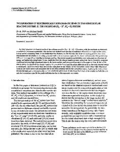
350 2.2. The Ocean Model PomCFS uses a bottom following sigma-coordinate vertical grid, a coastal-following curvilinear orthogonal horizontal grid, and includes a turbulence sub-model (Mellor and Yamada, 1982). These model attributes make it attractive for coastal modeling. The model is robust in dealing with large variations of bottom topography (Ezer, 1994; Mellor et al., 1994) which are important in the coastal zone adjacent to the deep open ocean. The prognostic variables of the model are the free surface elevation, potential temperature, salinity (hence density using the equations of state modified from the UNESCO formulas by Mellor, 1991), and velocities. The numerical scheme has a split time step, i.e. an external mode which solves the vertically integrated momentum equation and an internal mode which solves the three-dimensional momentum, heat and salt equations. Horizontal diffusion is based on the so-called Smagorinsky formulation, i.e. it depends on grid size and velocity gradients and is applied along sigma levels (Mellor and Blumberg, 1985). For further details on the numerical scheme see the Princeton Ocean Model Users Guide (Mellor, 1992) and the papers cited above. The model grid and bottom topography, H(x,y), for the east coast region are shown in Figure 1. This grid is an extension of the Gulf Stream model, initially developed at Princeton University and Dynalysis of Princeton and used by Mellor and Ezer (1991) and Ezer and Mellor (1992) for data assimilation and Gulf Stream separation studies, respectively. The present domain has also been used by Ezer et al. (1992; 1993); Ezer and Mellor (1994); and Ezer (1994). The model has 15 sigma levels, sigma = (z - rl)/(H + 11), in the vertical (0, -0.004, -0.01, -0.02, -0.04, -0.06, -0.08, -0.1, -0.12, -0.16, -0.24, -0.4, -0.6, -0.8, - 1), and 181 x 101 horizontal grid points with a resolution of 10 to 20 km.
Figure 1. The (A) pomCFS model grid, with fixed transport (in Sverdrups) boundary conditions as indicated and (B) the model bottom topography (contour interval is 200 m) based on the U.S. Navy DBDB5 (5 minute gridded) data. The coastal boundary of the model is at 10 m depth on the continental shelf.
351 For the external mode (the vertically integrated equations of motion), the open ocean boundary conditions are specified (see Figure 1) as follows: Near the south-west comer of the model, at the Florida Straits, a total inflow transport of 30 Sverdrups (1 Sverdrup = 106 m3sec ~) is prescribed and is distributed horizontally according to measurements from the Subtropical Atlantic Climate Studies (STACS) program (Leaman et al., 1987). On the eastern boundary, the total of 90 Sverdrups is allowed to exit the domain between 37~ and 40~ while a total inflow of 30 Sverdrups enters north of the Gulf Stream, along the continental slope, and 30 Sverdrups also enters south of the Gulf Stream. The northern and southern inflows at the eastern boundary, which are based on a diagnostic calculation and observations, represent the northern recirculation gyre and the subtropical gyre, respectively. For the internal mode velocities, the open boundaries are governed by the Sommerfeld radiation condition. Therefore, although the total transport on the open boundaries is prescribed, the internal velocities are free to adjust geostrophically to the density field. An exception is the Florida Straits, where the internal velocities are also determined from the STACS measurements. On all open boundaries, temperature and salinity are prescribed from the Navy's observed climatology (used also for initialization), and are advected into the model domain whenever flow is into the domain.
2.3. The ECOFS System A schematic of the ECOFS system is displayed in Figure 2. In the forecast mode, daily 24hour 00Z pomCFS forecasts are run on the NCEP Cray YMP8. The operational Eta output (listed in Section 2.1) is interpolated in time from the three-hour Eta output interval to provide surface forcing at each pomCFS time step. A series of Eta 00Z forecasts for 6,9 ..... 27 hours is used, with the six-hour forecast being the first used to allow for adjustment of the Eta model. Figure 3 illustrates the ECOFS operational schedule. Daily pomCFS output fields include three-dimensional fields of temperature, salinity and velocities and two-dimensional surface elevation fields. Sea levels at selected model grid points, which are near NOS coastal water level gauge locations (see Section 2.4), are saved hourly. Restart files are produced every day to initialize the next day's forecast. Similar systems are also installed at Princeton and NOS for debugging, model development and sensitivity studies. The Princeton system runs on the Geophysical Fluid Dynamics Laboratory's Cray computer in a hindcast mode one month at a time, and the NOS system runs on an SGI Challenge L for experimental hindcast runs. Upon completing a forecast, postprocessed pomCFS surface field maps are printed automatically in a non-interactive manner; metafiles (NCAR graphics) are updated after each run and are available for ECOFS project members. In addition, graphics software has been developed for producing horizontal pomCFS output fields, accessible interactively through dialogue-type software, with interactively chosen options. This includes interpolation to Cartesian coordinates, mapping of selected scalar or vector two-dimensional fields and horizontal cross-sections of three-dimensional fields (either taken from standard model output or constructed by the user) defined on the ECOFS grid. A variety of software also exists for data processing, including calculation of spatial and temporal mean statistics and other integral properties. In addition, spatial and temporal interpolation of pomCFS velocity vectors to correspond to satellite feature tracking vector locations (see Section 3.3) is done as needed. Upto-date output fields are also available on the ECOFS homepage, accessible through the World Wide Web at http://www.aos.princeton,edu/htdocs.pom/CFS.
352
Figure 2. Schematic of the ECOFS operational system. Parts represented in green indicate operational functions; parts indicated in blue represent functions that are in transition to operations, such as runoff and E-P; and functions that are not yet operational (e.g. assimilation of SST and altimeter data; tides) are represented in red.
Figure 3. Schematic of the ECOFS operational schedule. The abscissa represents the Eta model schedule, including reinitialization of the model with all available data every six hours (large red dots) and running of 48-hr Eta forecasts every 12 hours (diagonal blue lines). The ocean model (pomCFS) 24-hour forecasts are run once a day, using surface fluxes from the Eta model at hours 6,9 ...... 27.
353
2.4. Data Sources For Evaluation And Assimilation Water Level Data For many users of ECOFS information, coastal sea level is one of the most important parameters to be predicted. Thus, forecasting routine changes in coastal sea level, as well as those associated with storm surge, is a high priority of the ECOFS, and observations of sea level from coastal water level gauges are a primary source of data for evaluation of the system. There has been a special effort to establish near-real-time access to the NGWLMS data available from stations along the east coast of the U.S. The individual water level gauge data are transferred via the satellite-based GOES data collection system to the Wallops Island data acquisition station to files processed by NOAA's Ocean Products Center, and then to the NCEP Cray where the model forecast fields reside. The water level data are obtained from the stations indicated in Figure 4, which include eighteen NGWLMS gauges and two Canadian gauges (Halifax and St. Johns) which are transmitted via internet from the Canadian Marine Environmental Data Service on a daily basis. The NGWLMS data are updated every three hours (i.e. at 03:00, 06:00 .... ) and include sixminute water levels referenced to mean sea level, astronomical tidal residuals, back-up water level sensor readings, standard deviations, and number of outliers, as well as hourly sea level pressure, air and sea surface temperature, and wind speed and direction. The NGWLMS data used for evaluation of the first 12 months of operational coastal water level prediction are described in Section 3.1. Sea Surface Temperature Satellite-derived SST fields are obtained from the Advanced Very High Resolution Radiometer (AVHRR) on board NOAA's polar-orbiting satellites. These data sets are important for evaluation of the model SST and the atmosphere-ocean heat budget. Experiments show that SST data can be assimilated into the model in conjunction with altimeter data (Ezer and Mellor, 1995), which may improve nowcasts for areas where the altimeter data is less accurate, such as close to the coast. Analyzed 14-km gridded MCSST data are available from NESDIS and are currently being used for evaluation purposes. Altimetry Data Observations of sea surface height of the world oceans by satellite altimeters provide a vast amount of data for evaluation of ocean models and assimilation into models. The long-term data from the GEOSAT altimeter, which operated between 1986 and 1989, have been used to examine ocean variability and in the development of different techniques for the use of this data in conjunction with ocean models. In particular, such data have been used to develop data assimilation techniques (described in more detail in section 5.4) for the Princeton ocean model. Nowcast/forecast experiments (Mellor and Ezer, 199 l; Ezer et al., 1992, 1993; Ezer and Mellor, 1994) using data assimilation procedures show considerable skill in the prediction of the Gulf Stream and eddy variabilities, whereas data assimilation was less effective in the near-coastal region where the altimeter was less reliable. New data from the TOPEX/Poseidon altimeters, launched in 1992, have much better accuracy than previous altimeters. Other satellites, such as the ERS-l, are presently available for ECOFS and the ERS-2 has already been launched and may soon replace the ERS-1 as an altimetry data source. Through a joint agreement with the U.S. Navy (NAVOCEANO, Stennis
354
Figure 4. Network of coastal water level stations used in the ECOFS. The two Canadian stations (St. Johns and Halifax) are provided by the Canadian Marine Environmental Data Service (MEDS) and the U.S. stations are part of the NOS real-time NGWLMS.
Space Flight Center, MS), ECOFS will obtain the TOPEX/Poseidon and the ERS-1 altimetry data in near-real-time. Satellite altimeters measure sea surface height along the satellite tracks, which have regular repeat cycles. In the case of TOPEX the repeat cycle is 10 days. For comparison, the repeat cycle was 17 days for GEOSAT and is about 35 days for ERS-1. In
355
addition, high quality analyses of complete two-dimensional elevation fields, after atmospheric and oceanic corrections and calibrations have been applied, are also available now (King et al., 1994; Stammer and Wunsch, 1994). A major challenge will be to make such analyses available in real-time for direct assimilation into the operational ocean model. The primary use of the altimeter data will be to constrain the Gulf Stream to its observed locations; in the current operational model, the Gulf Stream is free to meander due to its intrinsic instability, and thus its location at any given time will differ from the observed location.
Surface Currents Estimates of surface currents can be obtained from satellite feature tracking techniques. Sequential SST imagery derived from satellite-borne AVHRR sensor data has been used to estimate surface currents in a variety of coastal areas around the continental U.S. (Koblinsky et al., 1984; Holland and Yan, 1992; Kelly and Strub, 1992). The possibility of using sequential satellite imagery for estimating surface flows on an operational basis is presently being explored (Breaker et al., 1994a,b), and efforts are also being made to utilize ocean color data from the Sea-Viewing Wide Field-of-View Sensor (SeaWiFS) and the Ocean Color and Temperature Scanner (OCTS) on the Japanese ADEOS polar-orbiting satellite to conduct feature tracking in support of the ECOFS. Ocean color may serve as a better tracer of the circulation, particularly in areas where sediments, yellow substance and detritus are plentiful. Some preliminary comparisons between ECOFS surface currents and feature tracking-based surface currents in the Middle Atlantic Bight are described in Section 3.3. Florida Straits Transport The present operational model uses a constant inflow of 30 Sverdrups in the Florida Straits. However, estimates of this transport can be obtained from voltage differences measured along an in-service Florida-Bahamas submarine cable straddling the Straits at about 27~ (Larsen, 1992). Hourly mean voltage data are processed to remove the geomagnetic signal and the tides, and the hourly values are then used to compute daily mean transports of the Florida Current. In a hindcast mode we are using this information to evaluate the impact of variable transport (inflow) at the southern boundary over the entire model domain (see Section 4.6), and the possibility exists to use this data operationally to provide the observed inflow boundary conditions.
3.
EVALUATION
3.1. Subtidal Water Level Initial assessment of the ocean model skill is done through comparison of the 24-hour forecast subtidal water level at the model's shoreward boundary to observations along the coast (Bosley and Aikman, 1994). Twenty coastal real-time water level stations (eighteen from the NGWLMS and two from the Canadian Marine Environmental Data Service), including locations from Florida to Newfoundland, are being used for this assessment (Figure 4). Results from comparisons of one year of data between September 1993 and August 1994 are discussed here. For the twelve month period all the forecast and observed records have had the mean removed and were then subjected to a 30-hour low pass filter.
356 The comparisons show that nearly each subtidal event which is present in the winter observations is also manifest in the forecast sea level, although some phase and amplitude differences exist (see Figure 5 for some comparisons). Seasonal differences, with lower subtidal sea level variability in the spring and summer and higher variability in the fall and winter are well represented in the model. The forecasts at the two open ocean stations (Bermuda and Settlement Point, Bahamas) show very little subtidal (wind-driven) variability, but the inclusion of atmospheric pressure effects (see Section 4.2) will improve these comparisons considerably. For this twelve-month period, the observed and forecast water levels have a meridional average correlation coefficient of 0.65 and an rms difference of 10 cm (see Table 1). The comparisons suggest that the difference between forecast and observed subtidal water level is greatest in the southern Middle Atlantic Bight and that the smallest differences are found in the Gulf of Maine (Figure 6). An examination of the ratio of the forecast-to-observed standard deviations (Table 1) also indicates that the ocean model under-represents subtidal variability, on average, by less than 40% (Figure 6). Efforts to improve the forecast skill for coastal water levels through possible enhancements to both the Eta and pomCFS models are underway. For example, there is some indication that the Eta model wind drag coefficient (and thus wind stress) is too low, especially at wind speeds between 2 and 12 m s -~, thus alternative momentum flux formulations are being examined. Also, the current operational ocean model grid does not extend to the coast because its shoreward boundary is at about the 10 m isobath. As a result, we are comparing forecast water levels at grid cells that can be significantly different (both in distance and in terms of the water depth) from the site of the coastal water level station. To further test the sensitivity of the forecasts, experiments with refining the grid resolution near the coast and incorporating more accurate and higher resolution bathymetry to better represent local conditions are underway.
3.2. Sea Surface Temperature At this time only qualitative comparisons between forecast and observed SST from satellite AVHRR images are done on a regular basis. In the future an operational quantitative evaluation will be performed as well. The qualitative comparisons have indicated problems in the air-sea heat fluxes and possibly in the ocean model vertical mixing. In particular, comparisons made during the summer reveal that the model surface temperatures are too high. It has been determined that the Eta model surface heat fluxes differ considerably from climatology (see Section 4.1) and thus do not allow the Gulf Stream to cool sufficiently. By calculating the surface heat fluxes using the Eta lower layer fields (i.e. air temperature, wind speed, humidity, etc.), instead of directly using the Eta model heat fluxes (as is done in the present operational version), the forecast surface temperatures improve considerably. As an example, a comparison between the observed and model surface temperatures is shown in Figure 7. The upper panel is the MCSST image obtained from a 14-km resolution analysis based on satellite data collected between February 27 and 28, 1995 and interpolated onto the pomCFS grid. The middle panel is the February 28, 1995 forecast SST obtained from the experimental ECOFS, where surface heat and momentum fluxes are obtained directly from the Eta model. The lower panel is the forecast SST for the same date obtained from an updated version of the ECOFS, where surface heat and momentum fluxes are calculated from the lower layer atmospheric Eta fields. Note the better agreement between the updated ECOFS and the MCSST, as compared to the experimental ECOFS. For example, in the updated ECOFS cold shelf water penetrates further south into the southern Middle Atlantic Bight, as observed; the
357
NORTH 2.45
2.10 1.75 .
Halifax Eastport Portland Boston
1.40 _~
1.05 0.70
--0.35 .
--0.70
.
.
.
.
.
.
.
.
.
.
.
.
.
.
.
.
.
1o
z
JANUARY
FEBRUARY 1994
MIDDLE
-t~
3.50 3.15 2.80 2.45 2.10 . 1.75 1.40 1.05 0.70 0.35 0 --0.35 --0.70
Newport Montauk Sandy Hook Atlantic City Lewes CBBT Duck . . . .
;3A I~JA~I Y . . . . . . . . . . . 1994
F~BI~JA~Y . . . . .
SOUTH
..~
3.15 2.80 2.45 2.10 1.75 1.40 1.05 0.70 0.35 0 --0.35 --0.70
Wilmington Springmaid Ft. Pulaski St. Augustine Settlement Pt Bermuda ,
4
;,
,o
,s
1.
,i.
JANUARY
== zs 21l 31
~l
.
i
lZ
~
11l
;I,
a.l
~r/
z
FEBRUARY
1994
Figure 5. A two month (January and February 1994) sample of comparisons between the forecast (dashed lines) and observed (solid lines) subtidal water level at the East Coast stations indicated.
358
Table 1 Statistics based on 12 months (1 September 1993 to 31 August 1994) of observed and 24-hour forecast subtidal water level. Presented are the observed and forecast standard deviation, the ratio of these two, the rms difference, and the correlation coefficient at the coastal stations indicated. STATION
Stand. Dev. Obs (m)
Stand. Dev. Model (m)
Ratio Mod/Obs
RMS Diff (m)
Correlation Coefficient
Eastport
0.123
0.066
0.534
0.093
0.570
Halifax
0.112
0.063
0.567
0.089
0.521
Portland
0.128
0.075
0.589
0.087
0.653
Boston
0.136
0.083
0.605
0.089
0.688
Newport
0.134
0.089
0.661
0.082
0.740
Montauk
0.135
0.109
0.812
0.085
0.759
SandyHook
0.185
0.127
0.684
0.102
0.800
Atlc
0.178
0.118
0.664
0.108
0.743
Lewis
0.179
0.126
0.705
0.110
0.747
CBBT
0.165
0.108
0.655
0.125
0.596
Duck
0.164
0.078
0.479
0.130
0.486
Wilmington
0.116
0.086
0.744
0.105
0.468
Springmaid
0.153
0.089
0.583
0.105
0.649
Bermuda
0.090
0.042
0.466
0.102
-0.020
Ft. Pulaski
0.173
0.109
0.628
0.103
0.745
St. August
0.164
0.093
0.564
0.105
0.691
Settlement
0.088
0.038
0.425
0.109
-0.282
359
,.~ z
4o
--7 . . . .
9 ' " HALI',F~'EAST . . . . . BO_ST~ PORT NEWP ~_.__ SAND MONT ~',,,,t=AT LC
* 'EASI~~I['HILI' PORT
WILM ~ " ' ~ ' ~ BERMZ SPRI "~ FTPU
13
"6 _..J
STAU ~ 25 O. 06
.
i
,
i
0.08
,
1
,
i
,
:
.
0.10
RMS Difference(m)
~CBBT
S P R ~ BERM
WlLM
~ - ~ FTPU
SETT i
' #
MONT/e~~"~N D A T L C ~ LEWS DUCK
35
'
BOST " ' , , - ~ . E L
(::3
_~
'
i
0.12
SETT S .
9
i
0.1
,
i
0.2
9
1
0.3
,
|
0.4
.
1
0.5
,
1
0.6
,
1
0.7
,
|
0.8
.
0.9
Modelled SD/Observed SD
Figure 6. RMS difference (left) and the ratio of forecast to observed standard deviations (fight) at the indicated East Coast stations for the 12-month period, September 1993 to August 1994.
surface temperatures in the Gulf Stream and the subtropical gyre are colder and in better agreement with the MCSST data; and cold water indications of upwelling over the South Atlantic Bight shelf and very cold temperatures on the Newfoundland shelf are also apparent now, as observed. In general, and despite the fact that, without data assimilation, the Gulf Stream and other fronts in the model are not expected to be at their observed locations, considerable agreement in the SST structure is seen.
3.3. Feature Tracking Nowcasting and forecasting reliable information on ocean surface currents is clearly an important goal of the ECOFS, but virtually no real-time data are available to define the surface current field. Independent information on surface flow, if it were available, would provide valuable input to the ECOFS, both for model evaluation and for assimilation into the model. Satellite feature tracking techniques offer such an opportunity. In feature tracking, the displacements of selected thermal features are determined from precisely co-registered SST images which are approximately 12 to 24 hours apart. If the motion is assumed to be purely advective and rectilinear, estimates of the surface flow can be obtained by dividing the measured displacements by the time intervals between the images. As a result, the technique is essentially Lagrangian. This approach has been used successfully by meteorologists to estimate low-level winds from geostationary satellite data for the past 25 years. For the oceanic case, both manual and automated methods of feature tracking are employed, although manual feature tracking is not objective, and automated methods often lack resolution. Feature tracking methods have been slow to emerge in oceanography because of uncertainties in using SST as a tracer of the flow and because there is the requirement for highly accurate earth-location for the satellite imagery (i.e. the feature displacements between successive
361
satellite fixes are often relatively small, on the order of tens of kilometers or less). Although feature tracking has a number of limitations, overall it has been rather effective in capturing the general character of the prevailing flow in areas where adequate distributions of thermal features are present. Figure 8 shows a surface current analysis based on satellite feature tracking for a portion of the Middle Atlantic Bight. Two AVHRR images approximately 12 hours apart on 10 May 1993 were used in this analysis. The surface flow vectors have been smoothed slightly to emphasize the synoptic-scale circulation. Southwestward flow over the continental shelf and slope shoreward of the Gulf Stream is clearly evident, as well as the entrainment of shelf and slope water along the north wall of the Gulf Stream just northeast of Cape Hatteras. These results are qualitatively consistent with historical moored and drifter current meter observations in this region (Csanady and Hamilton, 1988; Aikman and Wei, 1995). Surface currents based on feature tracking, such as the example shown in Figure 8, have been compared with the ECOFS model forecasts on several occasions in the slope water region between 35 and 40 ~ N (Breaker et al., 1994b). In contrast with the ECOFS 24-hour forecasts, which showed a lack of southwestward flow in the shelf and slope water region, the satellite-derived flows showed consistent flow to the southwest in this area. These comparisons have also indicated the difficulties inherent in making unambiguous comparisons between independent sources of data. Experience has shown that feature tracking methods which employ infrared satellite data often tend to underestimate the speeds of surface currents, particularly in areas of jet-like flow (e.g. Kelly and Strub, 1992). It will be important in the future to obtain additional in situ surface current data to determine where, and under what conditions, such biases occur and to quantify these biases so that adequate corrections can be made. The present limitations in feature tracking require improved methods for the use of satellite-derived estimates of surface currents and the displacement of features in an assimilative capacity in ECOFS, but the information contained in and the spatial coverage possible from feature tracking is of great value for evaluation purposes.
4.
SENSITIVITY STUDIES
4.1. Surface Boundary Conditions As described in Section 3.2, during the summer the surface temperatures in the ocean model were found to be too high when compared with observations; the area-averaged model SST was as much as 3~ higher by mid-summer. An examination of the Eta model wind stress and comparisons between climatological and Eta model heat fluxes led to the realization that the Eta model uses drag coefficients that are too low and that the Eta model produces excessive oceanic surface heating. With the exception of the long wave radiation from the surface of the ocean, which depends on the ocean model SST, in the operational system the heat fluxes from the atmosphere to the ocean are derived solely from the Eta model. However, if we use the Eta lower layer fields to calculate the surface heat fluxes, instead of directly using the Eta model heat fluxes, the forecast SST improves considerably (see Figure 7 and Section 3.2). The procedure for doing this involves two steps. First, we employ corrected surface bulk coefficients to calculate new momentum, latent heat and sensible heat fluxes, and second, we then correct each of the Eta model surface heat flux components with simple constants so as to approximately match
362
..I
p~ORBITS-, "23833
RES- 1,47KM
4
J 34,5N 70,8W
Figure 8. Two AVHRR satellite images approximately 12 hours apart from 10 May 1993 were used to produce these estimates of surface flow in the southern portion of the Middle Atlantic Bight. The origins of each vector are plotted at the mid-points between the two feature locations. The flow field shown has been smoothed slightly to emphasize the synoptic-scale flow pattern. climatology. As the Eta model improves independently of the ECOFS, these constants will progress towards the value of unity, but in the meantime this allows us to capitalize on the temporal and spatial variability provided by the Eta model. This corrective action is illustrated in Figure 9, where the 1994 spatially and monthly averaged Eta model net heat fluxes (before and after correction) are compared with the climatology of Oberhuber (1988). Note that the annually averaged operational Eta model net heat flux is too warm by about 100 W m 2.
363
300
i
,
Net Heat Fluxes w ,
w
|
200 100 E
0 84 -100 -200
iETA.cor:
~. , , ~ _ ~
"3000
4 Month
Figure 9. Comparison of 1994 spatially and monthly averaged net heat fluxes from the COADS climatology (Oberhuber, 1988), the operational Eta model, and the corrected Eta fluxes. The short horizontal lines on the right are annual mean values.
4.2. Atmospheric Pressure Loading The current ocean forecast system is driven at the surface by wind stress and heat fluxes which are obtained from the Eta regional atmospheric model. As shown in Section 3.1, at most coastal stations subtidal variations in sea level are driven primarily by the wind stress; thus the comparison between forecast and observed sea level is quite good, in spite of model and data deficiencies and the lack of any data assimilation. Another source of surface forcing that is currently not included in the ECOFS is atmospheric pressure loading that affects the adjustment of the sea surface of the ocean. The static response of the ocean to atmospheric pressure forcing is the so-called "inverted barometer effect", but there is also a dynamic response due to the spatial distribution of atmospheric pressure. A recent study by Pont (1994) indicates that on time scales shorter than about three days the dynamic effect of atmospheric pressure may be as important as the wind stress. To improve sea level nowcast/forecast skill in the ECOFS, the effect of sea surface atmospheric pressure (SSP) loading has recently been tested. Two parallel calculations, with and without SSP, were performed for a two-month period from December, 1993 to January, 1994. Comparing the two runs at Eastport, ME and Bermuda (Figure 10), we note that (a) the difference in sea level variability increases from south to north due to the stronger pressure variability in the north, and (b) the difference near the coast is relatively small, which suggests that coastal sea level variation is primarily driven by the wind stress. The calculated water levels without SSP compare fairly well with observations at the coast, although the calculation with SSP shows some improvement. A far greater improvement is obtained at Bermuda (Figure 10). As noted in Section 3.1, without SSP the model sea level exhibits very little subtidal variability at an open ocean site such as Bermuda. With SSP, the model sea level displays a good phase relationship with the observations and reaches about 70% of the observed variability. In general, the study reveals that the model results, although improved when atmospheric pressure loading
364
EASTPORTI 0.6
i
i
,
1
,
i
0.4 ..
oI
1
-0.2
-0.4
-0.(]; 330
I 340
a 350
, 360
J 370
, 380
390
,
|
400
BERMUDA 0.2
=
i
=
0.4
0.2
E
,, '.
-
A
_
..'-
.
o
II
i
t..~I
"i'---'-
-0.2
-0.4
-0.6 330
' 340
~ 350
' 360
370
380
390
400
Day
Figure 10. Results of experiments including the effects of sea surface atmospheric pressure (SSP) on subtidal water levels at Eastport, ME (top) and Bermuda (bottom) for two months, December 1993 to January 1994. The observed water levels (solid lines) are compared to the forecast water levels with Eta model wind stress forcing only (dashed lines) and to the forecast water levels with Eta model wind stress forcing and SSP (dotted lines). Note the different scales on the ordinates.
365
is included, still have lower sea level variability than observed at all stations. The discrepancy could be due, in part, to an underestimate of wind speeds and pressure systems by the Eta model. In fact, recent results confirm that the Eta model produces wind drag coefficients that are too low, especially at wind speeds less than 12 m s -~. We are in the process of reformulating and testing new drag coefficients based on the Eta model wind speeds.
4.3. Lateral Boundary Conditions The presently experimental pomCFS contains fixed transport lateral boundary conditions, as explained in Section 2.2 (Figure 1), and relics on annual climatological temperature and salinity (based on the U.S. Navy's GDEM climatology) at all lateral boundary grid cell locations (ECOFS Group, 1994). The sensitivity of the ocean model to these open ocean boundary conditions may be considerable and this sensitivity is being examined in a number of ways. In the Florida Straits we are testing the model sensitivity to the measured inflow (see Section 2.4). Using the daily mean transports estimated from voltage differences measured along the in-service Florida-Bahamas submarine cable at 27~ a 12-month simulation is being examined for the impact of variations in the transport in the Florida Straits on downstream Gulf Stream behavior (transport, separation at Cape Hatteras, meandering) and coastal water levels. There has been some suggestion that seasonal water level fluctuations on the South Carolina shelf are associated with seasonal transports in the Gulf Stream (Noble and Gelfenbaum, 1992). East of the Bahamas on the model southern boundary we are testing the model sensitivity to recent estimates of transports in this region associated with the Antilles and Western Boundary Under Current (WBUC) systems (Lee at al., 1995). The pomCFS presently has zero transport prescribed across this boundary (Figure 1). The Antilles/WBUC numerical experiments change this to include: (1) the imposition of 5 Sverdrups input (Antilles Current) to the model domain from 0 to 800 m depth and 76 to 77~ (2) an export of 38 Sverdrups associated with the WBUC occurring at depths greater than 800 m over this same boundary segment; and (3) the allowance of two recirculation zones totaling 33 Sverdrups input to balance the net Antilles/WBUC output. Preliminary 12-month numerical experiments indicate that the sensitivity of coastal water levels to variable transport through the Florida Straits is minimal. Downstream coastal water levels, with the exception of the immediate vicinity of the Straits, do not appear to significantly respond to these variations. Likewise, subtidal coastal water level variations do not appear to be sensitive to the imposition of fixed Antilles/WBUC transports east of the Bahamas. The full impact of these transport changes at the southern boundary on coastal water levels, downstream Gulf Stream transports, position and separation at Cape Hatteras, as well as domain-wide SSE, SST and velocity fields is being examined. It is possible that we may need to extend these simulations beyond 12 months to thoroughly evaluate this impact. We are also testing the model sensitivity to imposing different estimates and distributions of the transport into the model domain on its eastern boundary, north of the Gulf Stream (currently fixed at 30 Sv). It is probable that the performance of the model in the Middle Atlantic Bight is sensitive to this. In addition to the transport boundary condition tests, we will test the model sensitivity to monthly climatological estimates of temperature and salinity at the model open boundaries. The pomCFS presently uses annual climatology and it is very likely that the monthly changes in the advective transports of heat and salt will be significant.
366
4.4.PredictabUity Studies Numerical experiments on predictability have been performed with the pomCFS (Sheinin and Mellor, 1994), wherein the output of the experimental, or "control" (CR) run, was compared with the output of another run of the same model, but with slightly different initial conditions. The "perturbed" (PR) run initial conditions are generated by imposing a small random perturbation on those of the control run. For both runs the same surface and boundary forcing was used. CR was started on 3 August 1993 with initial conditions taken from climatology. PR was started on 3 November 1993 using the results of the CR simulation for 15 November 1993 as initial conditions. The comparisons were made starting on the 59th day of the common period of the two runs, from 1 January 1994 to 31 December 1994, thus covering one year of model integration. The root mean square difference between the two runs is
RMSD--~ (a PR-a cR) 2 where a is any model property. The spatial distribution of RMSD for sea surface height and current speed is shown in Figures 1 l a and I lb. To quantify the predictability of the model system, a predictability index p is defined, such that
p:
(apR_aCR) 2
(acR_acR) 2+ (apR_apR) 2
which is just the mean square difference normalized on the sum of variances of the control run and the perturbed fields. For perfect predictability, p = 0. If the fields were unbiased (ideally, we should have longer runs) and uncorrelated such that (a cR-a cR) (a pR-a pR) --0
then it may be shown that p = 1, representing no predictability. The predictability characteristics were evaluated for model sea surface height and surface velocity. The results for the two fields are shown in Figures 11 c and 1 l d, where p is plotted on a logarithmic scale (c = log~0p). It is expected that p would be very low in shallow coastal regions, where the dynamics are dominated by the same wind stress forcing for each run, and this is what is seen in Figures 1 l c and 1 l d. Offshore in the Gulf Stream, where instabilities dominate, one expects p to be close to unity and this is also evident. Away from the Gulf Stream in open water, p for sea surface elevation is also close to unity. The variances are small, and most likely emanate from unpredictable Gulf Stream mesoscale variability. On the other hand, the surface velocity exhibits some predictability since surface wind stress is the dominant driving force of surface velocities in these regions. From these preliminary considerations, an obvious conclusion is that data assimilation is required for the Gulf Stream region. In the coastal ocean, the model is relatively deterministic, however it is worth noting that the full nowcast/forecast system will include wind stress errors that are not accounted for in this analysis.
367
Figure 11 a. Spatial distribution of the sea surface height RMSD between the two runs (control and perturbed) of the predictability study. The contour interval is 5 cm. The RMSDs are typically less than 5 cm (high predictability) everywhere, except for the Gulf Stream region, where values can exceed 25 cm.
Figure 11 b. Same as in Figure 11 a, but for surface velocity RMSD. The contour interval is 10 cm/sec. At the coast values are less than 10 cm/sec, but can exceed 50 cm/sec in the Gulf Stream region.
368
Figure 1 lc. Spatial distribution of the sea surface height predictability index, p. The data is plotted on a logarithmic scale, c = log~0p, contour interval of 0.5. Areas of high predictability (c < -1) are mostly coastal while c is close to zero in the Gulf Stream and open ocean.
Figure 11 d. Same as in Figure 1 lc, but for surface velocity predictability. As for sea surface height, coastal predictability is high (c < -1). In contrast to sea surface height, surface velocity exhibits some predictability in the open ocean.
369
5.
ENHANCEMENTS
5.1. Fresh Water Fluxes Although the ocean circulation in middle latitudes is generally affected more by variations in temperature than by variations in salinity, coastal regions such as the continental shelf near the mouth of bays and estuaries are significantly modified by fresh water fluxes, particularly during the spring period of high runoff. In the current ECOFS, variations in salinity are the result of advection and diffusion without any fresh water fluxes due to river runoff or evaporation and precipitation. Salinity at the open ocean boundaries is obtained from climatological data and is advected into the model domain during inflow boundary conditions (e.g. at the Florida Straits). Surface fresh water fluxes due to evaporation and precipitation (from the Eta forecasts) and from river runoff will be added in the near future. Initially, the major rivers along the U.S. and Canadian East Coast will be included by applying fresh water fluxes at the model grid points closest to each fiver mouth, using monthly climatological average runoff data. Further improvements may include the use of observed runoff data and an approach that also takes into account the effect of the inflow on velocities near the boundary. 5.2. Tidal Forcing A two-dimensional version of the Princeton ocean model has been modified to include astronomical forcing on open boundaries for the semi-diurnal (M2) and the diurnal (K~) tides. A least-squares optimization technique has been devised to solve for boundary tidal forcing by using observational tidal constants within the domain, mainly along the coast (Chen et al., 1995). The boundary forcing (elevation or depth-averaged velocities) is represented by a series of prescribed functions with unknown coefficients. These modes are correlated to model results within the domain through a response function which is determined by running the model. The optimal boundary forcing (mode coefficients) is obtained by minimizing the error between the model and the observations at tidal stations. When compared with results using boundary conditions driven by Schwiderski's (1980) global tidal model, the model results are improved when driven by the optimized boundary forcing. The more modes used, the smaller is the error, though five modes yield satisfactory results. The remaining model error is partly due to insufficient horizontal resolution and errors in the bathymetry. Future research will focus on further assessment of the tidal model results, inclusion of more tidal constituents, and incorporation of tidal forcing into the three-dimensional ECOFS model. 5.3. Thermal Expansion Effects In pomCFS, as well as in most other ocean models used today, volume rather than mass is conserved due to the Boussinesq approximation. Variations in sea level associated with expansion or contraction of the water column due to density changes are missing from ocean models. Recently, Greatbatch (1994) raised the concern that ocean models may not correctly simulate seasonal and climatic changes in sea level due to this omission. In fact, errors in the predicted sea level (Section 3.1) do indicate some long-term bias in the model sea level that we believe is associated with the missing expansion/contraction of the water column due to the seasonal heating/cooling cycle. In a recent study (Mellor and Ezer, 1995), the Princeton ocean model has been upgraded to remove the Boussinesq approximation so that the effect of thermal expansion is directly included in the model. A series of tests have been performed to evaluate
370 the differences between Boussinesq and non-Boussinesq calculations under different heating and cooling conditions and different model domains. The experiments show that the non-Boussinesq dynamics have only a minor effect on the baroclinic current field, and a small but non-negligible effect on sea level. Additional sources of error exist in regional models (both Boussinesq and non-Boussinesq) when the heating/cooling over the model domain is much different than that of the surrounding ocean and when open boundary conditions prevent transport through the boundaries. A spatially uniform time-dependent correction can improve sea level prediction in regional Boussinesq models; this correction will apply to seasonal sea level variability due to thermal expansion and concomitant transport across open boundaries. 5.4. Assimilation In recent years, considerable effort has been invested in developing data assimilation techniques for ocean models, with particular emphasis on nowcasting and forecasting the Gulf Stream system, where surface variations of satellite-observed fields are much larger than in any other area of the world ocean. There are two types of surface satellite data that may be useful for assimilation; SST data from the AVHRR sensor and Sea Surface Height (SSH) data from altimetry. However, a comparison of the two data types in the Gulf Stream region shows considerable differences due to differences in their spatial coverage (Ezer et al., 1993). Since satellite data primarily provide only surface information, efficient data assimilation must rely on the projection of the surface information into the deep ocean to update the three-dimensional oceanic fields. The assimilation scheme used with the Princeton ocean model is based on the methodology developed for altimeter data by Mellor and Ezer ( 1991) and Ezer and Mellor (1994). The main thrust of the scheme is the use of predetermined surface-subsurface correlation coefficients, C(x,y,z), and correlation factors, F(x,y,z), relating variations of the surface field's temperature anomaly, 6To(x,y), or elevation anomaly, 6rl(x,y), to variations of temperature and salinity at depth. These correlations are calculated from the model or from data. Higher correlations are obtained in the vicinity of the Gulf Stream and lower values are found in shallow regions and far from the Gulf Stream. At each assimilation time, the temperature TA (and similarly for salinity) used to initialize the next forecast is obtained according to T A= T M+ P(T c + Frrl - TM), where T Mis the model temperature field, T c is the climatological mean temperature, 611 is the observed anomaly SSH data and P is the weight. The same procedure can be applied to assimilation of SST where 61"1 is replaced by 6T Oand the appropriate correlation factor is used. The weights are calculated using an optimal interpolation approach that minimizes nowcast errors and takes into account model and data error estimates (see Mellor and Ezer, 1991 and Ezer and Mellor, 1994, for more detail). The spatial distribution of the weights also depends on the distribution of the correlation coefficient; thus, more weight is given to the data fields compared to the model fields in regions with high surface-subsurface correlations, such as in the vicinity of the Gulf Stream. A similar approach allows one to combine the two types of data, where the weights for each type of data depend on its error estimate. The experiments show considerable skill in nowcasting the location of the Gulf Stream front and its associated eddies, when compared with observations and analysis fields obtained from Navy sources (see Ezer et al., 1993 and Ezer and Mellor, 1994 for a description of the data used in the comparison). The average errors as a function of depth, shown in Figure 12, indicate that the assimilation of SST and SSH together yields smaller errors at all depths than the assimilation of each data type alone. In the upper layers, where T(x,y,z) is correlated better with To(x,y) than with rl(x,y), surface
371 temperature is a more effective source of data (see Ezer and Mellor, 1995 for more detail on these experiments), while in the deep ocean surface elevation is a more effective source of data. The data assimilation experience with the Princeton ocean model has been previously motivated by U.S. Navy interests in predicting variations in the Gulf Stream system. In the context of the ECOFS, the effort will focus on the coastal region and the transfer of techniques developed in a research environment to the operational system.
T E M P E R A T U R E ERRORS
!~ ~
-200
9
*"...., %~
..,.%.
;
-400
".~ I
9
Ill Q
Ii
-600
//,;
,,.,"
i
/
,
Auim. SST /b~im. SSH A==kn. SST+SSH NOA.r,sim.
-800
'/ I
I
- 1000 0.0
0.5
1.0 ERROR
1.5
2.0
2.5
3.0
(DEO)
Figure 12. Spatially-averaged temperature errors, as a function of depth, for ocean model runs with no data assimilation (thick solid line), SST assimilation only (closely dotted line), SSH assimilation only (dashed line) and assimilation of SST and SSH together (thin solid line) [from Ezer and Mellor, 1995]. 6.
D I S C U S S I O N AND S U M M A R Y
The ECOFS is a system that is under development and changes in the system can occur rapidly and frequently. A good example is the discovery of biases in the Eta model heat fluxes, based on comparisons with climatology, and indications that the Eta model wind stress is too low, especially at wind speeds of less than 12 m s -~. Based on this knowledge, recent and ongoing numerical experiments that use surface heat and momentum fluxes that are calculated based on the Eta model lower layer fields (instead of using the Eta fluxes directly) suggest significant improvements in the ocean model. A thorough evaluation of the impact of these changes on the ocean model are not yet available, but preliminary results show definite improvements in forecast SST values (Section 3.2). The lateral, as well as the surface, boundary conditions are being subjected to sensitivity tests (Section 4) and the results of these experiments will result in changes to the present transport open ocean boundary conditions. The inclusion of atmospheric pressure loading (Section 4.2), climatological fresh water fluxes from rivers (Section 5.1), and recent estimates
372 of the transport associated with the Antilles/WBUC (Section 4.3) are currently being tested operationally, along with the modifications to the surface heat and momentum fluxes. These changes will soon be implemented in the operational system. In addition, the results of further testing of the transport and annual climatological temperature and salinity open ocean boundary conditions, of including surface fresh water fluxes due to evaporation and precipitation, and of the tidal forcing (Section 5.2), will be evaluated and tested operationally. We are also testing a slightly revised pomCFS that includes more accurate and refined bathymetry over the continental shelf and shelf break (Section 3.1). These changes will also be implemented operationally once they have been tested and validated. To summarize, the Princeton ocean model is forced at the surface by fluxes of momentum and heat derived from the NCEP Eta model, to form the basis of the ECOFS operational system. Even though some biases exist in the Eta model fluxes, the initial 12 months of operational forecast subtidal water levels show remarkable and encouraging agreement with observations at the coast. The model SST shows phenomenological agreement with the observed SST fields, and it is found that using the Eta lower layer fields to calculate the surface fluxes, rather than directly using the Eta fluxes, improves the forecast SST considerably. Studies indicate high predictability near the coast, where the dynamics are dominated by wind forcing, and low predictability in the Gulf Stream region, where mesoscale variability and instabilities dominate. Comparisons with surface currents derived from feature tracking over the Middle Atlantic Bight shelf and slope indicate the model current field lacks the southwestward flow expected in this region. A series of enhancements, based on the results of a suite of sensitivity studies, are designed to improve the model forecasts and system before the implementation of observational data assimilation. Detailed data assimilation methodologies have been developed and near-real-time altimeter and AVHRR data are being prepared for operational assimilation, although initially they are being used for evaluation purposes in the ECOFS. Data assimilation experiments with the Princeton ocean model have historically focused on the Gulf Stream system, but in the ECOFS the focus will shift to the coastal region and to the operational application of these assimilation techniques.
7.
ACKNOWLEDGEMENTS
We wish to acknowledge the variety of personnel at NOAA and Princeton University who have contributed to the ECOFS project. At NOS, Charles Sun and John Cassidy have extended considerable effort to developing visualization software; Richard Schmalz is responsible for the open ocean lateral boundary condition sensitivity experiments; Eugene Wei has worked on developing an improved bathymetry and refined ocean model grid; and Phillip Richardson has contributed to the forecast coastal water level evaluation. Lech Lobocki has taken over the critical operational responsibility for the ECOFS model system at NCEP. At Princeton University, Namsoug Kim conducts many of the near-operational tasks and provides considerable programming support. We are also grateful to Jimmy Larsen, of NOAA's Pacific Marine Environmental Laboratory, for supplying us with the Florida-to-Bahamas telephone cable data, and a special thanks is extended to Brenda Via, of NOS, for her careful preparation of the camera-ready version.
373 The ECOFS Project is supported by the NOAA Coastal Ocean Program Office. The Princeton group has also been supported by the Office of Naval Research (the Navy Ocean Modeling and Prediction Program) and by use of the computational facilities of the NOAA Geophysical Fluid Dynamics Laboratory.
8.
REFERENCES
Aikman, F. III, G.L. Mellor, D.B. Rao, and M.P. Waters. 1994. A feasibility study of a coastal nowcast/forecast system. EOS, Transactions, American Geophysical Union, Spring Meeting, 75(16), April 19, Supplement, p 197. Aikman, F. III and E. Wei. 1995. A comparison of model-simulated trajectories and observed drifters in the Middle Atlantic Bight. Journal of Marine Environmental Engineering, in press. Black, T. L. 1994. The new NMC mesoscale Eta model: Description and Forecast Examples. Weather and Forecasting, 9, 265-278. Blumberg, A.F. and G. L. Mellor. 1987. A description of a three-dimensional coastal ocean circulation model. Three-Dimensional Coastal Ocean Models, 4, edited by N. Heaps., American Geophysical Union, 208p. Bosley, K. T. and F. Aikman III. 1994. Preliminary Comparisons of Forecast and Observed Subtidal Water Levels Along the U.S. East Coast. EOS, Transactions, American Geophysical Union, Spring Meeting, 75(16), April 19, Supplement, p197. Breaker,L.C., V.M.Krasnopolsky, D.B.Rao and X.-H. Yan. 1994a. The feasibility of estimating ocean surface currents on an operational basis using satellite feature tracking methods. Bulletin of the American Meteorological Society, 75, 2085-2095. Breaker,L.C., D.Sheinin and V.M.Krasnopolsky. 1994b. Estimating the surface circulation off the U.S. East Coast using sequential AVRRR satellite imagery in support of NOAA's emerging Coastal Forecast System. EOS, Transactions, American Geophysical Union, Spring Meeting, 75(16), April 19, Supplement, p197. Chen, P. and G.L. Mellor. 1995. Determination of tidal boundary forcing using tide station data. Submitted as a chapter in the book Coastal Ocean Prediction, C. Mooers, editor. Csanady, G. T. and P. Hamilton. 1988. Circulation of slope water. Continental Shelf Research, 8 (5-7), 565-624. ECOFS Group. 1994. A Coastal Forecast System: A collection of enabling information. Edited by T. Ezer and G. L. Mellor. Program in Atmospheric and Oceanic Sciences, Princeton University.
374 Ezer, T. 1994. On the interaction between the Gulf Stream and the New England seamount chain. Journal of Physical Oceanography, 24, 191-204. Ezer, T, and G. L. Mellor. 1992. A numerical study of the variability and the separation of the Gulf Stream induced by surface atmospheric forcing and lateral boundary flows. Journal of Physical Oceanography, 22, 660-682. Ezer, T. and G. L. Mellor. 1994. Continuous assimilation of Geosat altimeter data into a three-dimensional primitive equation Gulf Stream model, Journal of Physical Oceanography, 24, 832-847. Ezer, T. and G.L. Mellor. 1995. Data assimilation experiments in the Gulf Stream region: How useful are satellite-derived surface data for nowcasting the subsurface fields? Journal of Atmospheric and Oceanic Technology, in press. Ezer, T, D.-S. Ko, and G. L. Mellor. 1992. Modeling and forecasting the Gulf Stream, In: Oceanic and Atmospheric Nowcasting and Forecasting, D. L. Durham and J. K. Lewis (Eds.). Marine Technology Society Journal, 26(2), 5-14. Ezer, T, G. L. Mellor, D.-S. Ko, and Z. Sirkes. 1993. A comparison of Gulf Stream sea surface height fields derived from Geosat altimeter data and those derived from sea surface temperature data. Journal of Atmospheric and Oceanic Technology, 10, 76-87. Greatbatch, R. J. 1994. A note on the representation of steric sea level in models that conserve volume rather than mass. Journal of Geophysical Research, 99, 12,767-12,771. Holland, J.A. and X.-H. Yan. 1992. Ocean thermal feature recognition, discrimination, and tracking using infrared satellite imagery. IEEE Transactions on Geoscience and Remote Sensing, 30, 1046-1053. Kelly, K.A. and P.T. Strub. 1992. Comparison of velocity estimates from the Advanced Very High Resolution Radiometer in the coastal transition zone. Journal of Geophysical Research, 97, 9653-9668. Koblinsky, C.J., J.J. Simpson and T.D. Dickey. 1984. An offshore eddy in the California Current System. Progress in Oceanography, 13, 51-69. King, C., D. Stammer, and C. Wunsch. 1994. The CMPO/MIT TOPEX/POSEIDON altimetric data set. Department of Earth, Atmosheric and Planetary Sciences, MIT, Report No. 30, 42pp. Larsen, J.C. 1992. Transport and heat flux of the Florida Current at 27~ derived from crossstream voltages and profiling data: theory and observations. Philosophical Transactions of the Royal Society of London, 338, 169-236. Leaman, K. D., R. L. Molinari and P. S. Vertes. 1987. Structure and variability of the Florida Current at 27~ April 1982-July 1984. Journal of Physical Oceanography, 17,565-583.
375
Lee, T. N., W. Johns, R. Zantopp, and E. Fillenbaum. 1995. Moored Observations of Western Boundary Current Variability and Thermohaline Circulation at 26.5 ~ N in the Subtropical Atlantic. submitted to Journal of Physical Oceanography. Mellor, G. L. 1991. An equation of state for numerical models of oceans and estuarines. Journal of Atmospheric and Oceanic Technology, 8, 609-611. Mellor, G. L. 1992. User's guide for a three-dimensional, primitive equation, numerical ocean model. Progress in Atmospheric and Oceanic Science, Princeton University, 35p. Mellor, G. L., and A. F. Blumberg. 1985. Modeling vertical and horizontal diffusivities with the sigma coordinate system. Monthly Weather Review, 113, 1380-1383. Mellor, G. L., and T. Ezer. 1991. A Gulf Stream model and an altimetry assimilation scheme. Journal of Geophysical Research, 96, 8779-8795. Mellor, G. L., and T. Ezer. 1995. Sea level variations induced by heating and cooling: An evaluation of the Boussinesq approximation in ocean models. Journal of Geophysical Research, in press. Mellor, G. L., T. Ezer and L. Y. Oey. 1994. The pressure gradient conundrum of sigma coordinate ocean models. Journal of Atmospheric and Oceanic Technology, 11, 1126-1134. Mellor, G. L., and T. Yamada. 1982. Development of a turbulence closure model for geophysical fluid problems. Reviews of Geophysics and Space Physics, 20, 851-875. Nobel, M. A. and G.R. Gelfenbaum. 1992. Seasonal fluctuations in sea level on the South Carolina shelf and their relationship to the Gulf Stream. Journal of Geophysical Research, 97(C6), 9521-9529. Oberhuber, J. M. 1988. An atlas based on the COADS data set: the budgets of heat, buoyancy and turbulent kinetic energy at the surface of the global ocean. Max-Planck lnstitut fur Meteorologie, Report No. 15. Ponte, R. M. 1994. Understanding the relation between wind- and pressure-driven sea level variability. Journal of Geophysical Research, 99, 8033-8039. Schwiderski, E.W. 1980. On charting global ocean tides. Reviews of Geophysics and Space Physics, 18(1), 243-268. Sheinin, D.A. and G.L. Mellor. 1994. Predictability Studies with a Coastal Forecast System for the U.S. East Coast. EOS, Transactions, American Geophysical Union, Spring Meeting, 75(16), April 19, Supplement, p 197. Sheinin, D.A. and D.B. Rao. 1995. A Coastal Forecast System for the U.S. East Coast: Ocean Model Systematic Errors and Vertical Mixing Parameterization problem, WMO/ISCU, CAS/JSC
376 Working Group on Numerical Experimentation, Research Activities in Atmospheric and Oceanic Modeling, Rep. #20. Stammer, D. and C. Wunsch. 1994. Preliminary assessment of the accuracy and precision of TOPEX/POSEIDON altimeter data with respect to the large scal ocean circulation. Journal of Geophysical Research, 99(C 12), 24,584-24,604.