prohibitively expensive programming e orts. It would also smooth the steep learning curve often faced by novice users of data mining tools and libraries. Finally ...
Towards Automated Synthesis of Data Mining Programs Wray Buntine� Dept. of EECS, UC Berkeley Berkeley, CA
Abstract
Code synthesis is routinely used in industry to generate GUIs, form lling applications, and database support code and is even used with COBOL. In this paper we consider the question of whether code synthesis could also be applied to the data mining phase of knowledge discovery. We view this as a rapid prototyping method. Rapid prototyping of statistical data analysis algorithms would allow experienced analysts to experiment with di�erent statistical models before choosing one, but without requiring prohibitively expensive programming e�orts. It would also smooth the steep learning curve often faced by novice users of data mining tools and libraries. Finally, it would accelerate dissemination of essential research results and the development of applications. In this paper, we present a framework and the basic software for the automated synthesis of data analysis programs. We use a speci cation language that generalizes Bayesian networks, a popular notation used in many communities. Using decomposition methods and algorithm templates, our system transforms the network through several levels of representation and then nally into pseudocode which can be translated into the implementation language of choice. Here, we explain the framework on a mixture of Gaussians model, a core data mining algorithm at the heart of many commercial clustering tools. We mention the e�ectiveness of our framework by generating pseudocode for some more sophisticated algorithms from recent literature.
�Funded by a NASA Universities Grant 05106. yResearch Institute for Advanced Computer Science. zRecom Technologies, Inc.
Bernd Fischeryand Thomas Pressburgerz NASA Ames Research Center Mo�ett Field, CA
1
Introduction
A key component of the data mining task within knowledge discovery is statistical data analysis. Applied and computational statisticians who perform this task on smaller data sets use experimentation with di�erent statistical models and development of specialized algorithms to achieve reliable and useful results, especially in situations where the data cannot be cast into a form suitable for one of the standard algorithms. This capability is not practically availiable to the knowledge discovery community. In this paper we develop an alternative approach to rapid prototyping of data mining tools based on program synthesis, the derivation of a program that meets a given speci cation. We apply these methods to synthesize data analysis programs from Bayesian network speci cations using a library of e�cient algorithm templates together with core special-purpose algorithms and general purpose solvers, related to a suggestion from [3]. We show that this approach can address nontrivial data analysis problems. Our approach is motivated by three observations. First, the success of BUGS [16] demonstrates the need for data analysis tools suitable for reliable rapid prototyping. Second, Bayesian networks provide a ready, unifying speci cation language, as seen by their widespread use in communities such as applied Bayesian statistics and neural information processing [17, 8]; their role for the data mining community is to provide a exible data modeling language [4]. Finally, program synthesis has been proven to be competitive in other domains. It o�ers: �
�
�
Rapid turn-around : even for large tasks mature synthesis systems usually require less than a few minutes to produce code [11, 2]. Reliability : synthesized code is used in production systems to schedule military logistics [2] or to price stock options [15]. E�ciency : synthesized code can be an order of magnitude faster than hand-crafted special-purpose
code [2]. However, to the best of our knowledge, program synthesis has not previously been applied to data analysis algorithms; an edited discussion on its relevance appears in [5]. Speci c advantages for data analysis, other than rapid prototyping, are that generated code should be time and space e�cient; to achieve this we would rely on high-performance optimizing compiler techniques [1] coupled to our pseudo-code, as discussed in Section 3.2.
2
2.1
Preliminaries
A simple problem
As a simple running example to illustrate our concepts we will use mixture of Gaussians (cf. Fig. 1). It is covered in detail in many statistical texts, e.g., in [3]. This is a model for the measured data vector ~x based on parameter vectors �~; �~ ; ~� that are to be estimated. Figure 1(a) shows a two dimensional version of the σ
11 00 Gauss 00 11 x 00 11 00 11
c
ρ
1
200
Figure 1: A mixture of Gaussians: data and model problem where each Gaussian can be fully covariate. Here, example data is represented with a scatter plot; projections of the component Gaussians that make up the distribution are shown on both axes. The dots are roughly clustered in four blobs: top left, bottom right, bottom left, and a diagonal blob. Hence, C , the number of Gaussians being \mixed", is four. The Bayesian network for the model is given in Fig. 1(b). Bayesian networks are acyclic directed graphs that de ne probabilistic dependencies between variables; we assume the reader is familiar with them.1 The box placed around the variables c and x indicates that they are vectors of data where each of the 200 components is independently and identically distributed. The vector ~c (the \hidden variable" of the model which captures the assignment of the dots to the blobs) is discrete, with each entry taking a value f1; 2; :::; C g, and the vector ~x is real valued. The full joint probability for this model is P r(�) P r(� ) P r(� j � )
Y P r(c j �) P r(x j �[c ]; �[c ]) ; 200
i
i
i
i
i=1
where � parameterizes the discrete distribution over each discrete value c for i = 1; : : : ; 200, and (�[j ]; �[j ]) are the Gaussian parameters for each of j = 1; : : : ; C i
1
N i
i
Tutorials and references can available at www.auai.org.
i
i
C
i
j
i
i;j
µ 1
Gaussian peaks in the data. The precise form of the prior distributions for �; �; � is left unspeci ed here; they could be considered as variables for a maximum likelihood analysis, or be fully speci ed for a Bayesian analysis. An intuitive interpretation of this mixture model is that we rst generate data from C individual Gaussians, mix up these data according to the proportions given by �, and throw away the information regarding the original Gaussian source. This kind of problem is traditionally handled using an algorithm known as Expectation-Maximization (EM); our presentation follows [12]. In the mixture of Gaussian problem, one common interpretation of the P learning task is to seek to maximize =1 log P r(x j � ~; � ~; ~ � ). The problem here is that the inner probabilities are themselves over c , P r(x j �~; �~ ; ~� ) = P =1 P r(x ; c j �~a; �~sum ;~ � ), and the combination with the log makes the formula intractable. To overcome this, a new set of parameters is introduced and a cyclic \reestimation" method is used as follows: 1. Set q = P r(c = j j x ; �~; ~�; ~� ) for i = 1; : : : ; N and j = 1; : : : ; C . Thus ~ q is a discrete distribution on ~c. 2. Maximize E � [log P r(~x; ~c j �~; ~�; ~�)] for �~; ~�; ~� given ~ q above. Here, the log probability is evaluated according to the correct model, and then ~c is quanti ed out by averaging using ~q. This EM algorithm applies for these general probability forms, and not just the mixture of Gaussians. i
~ c
2.2
i
q ~
Indexed variables, Bayesian networks
In data analysis, indexed variables as vectors of data points, ~x = fx1 ; : : : ; x g with independent and identical distributions, or vectors of parameters �~ = f�1 ; : : : ; � g that behave similarly (e.g., di�erent nodes in a neural net) prevail. In Bayesian networks, such variables should not be \unfolded" (i.e., represented fully) because that obscures the model's regularities and increases the network's size. Instead, the network contains the most general representation and is unfolded only by demand and only locally. Hence, the representation must allow full vectors, ~x, generic single components, x , and particular single components, x5 . Our system uses Prolog-terms; a theory of indexed Bayesian networks, where indices are represented as Prolog variables is developed in [7]. The conditions required on the depends-literals2 are as follows: (1) each term in the second argument matches a term in the rst argument of some other depends-literals, (2) any variable in the second argument must appear in the rst, (3) the rst arguments for two di�erent literals cannot match, (4) the resulting graph is acyclic. N
C
i
2 depends(Var,VarList)
set of variables VarList.
says the variable Var depends on the
These conditions arise naturally from our speci cation language. We have extended Haddawy's results to work with non-ground probability queries since we seek to determine probabilities over indexed vectors. Tests for independence on these indexed Bayesian networks are easily developed in Lauritzen's framework which uses ancestral sets and set separation [9].
2.3
Expressions for probabilities
Given a Bayesian network, some probabilities can easily be extracted by enumerating the component probabilities at each node: Lemma 1 Let U; V be sets of variables over a Bayesian network with U \ V = ;. Then V \ descendants(U ) = ; and parents(U ) � V hold in the corresponding dependency graph i� the following probability statement holds: Y P r(U j V ) = P r(U j parents(U )) = P r(u j parents(u)) 2U
u
How can probabilities not satisfying these conditions be converted to symbolic expressions? Symbolic probabilistic inference [10], for instance extracts an e�cient expression for a particular marginal probability, p(U ). We have developed another result that lets us extract probabilities on a large class of mixed discrete and real, potentially indexed variables, where no integrals are needed and all marginalization is done by summing out discrete variables. We give the non-indexed case below; this is readily extended to indexed variables. Lemma 2 lets us evaluate a probability by a summaP 2Dom( 0 0 tion: P r(U j V ) = ) P r(U = u ; U j V ). Lemma 3 lets us evaluate a probability by a summation and a ratio: q (u) P r(U j V ) = P ; q (u) u0
P where q(u) =
U0
2Dom(U )
u
( = u0 ; U; V =V 0 j V 0 ). Lemma 2 V \descendants(U ) = ; holds and ancestors(V ) is independent of U given V i� there exists a set of variables U 0 such that Lemma 1 holds if we replace U by U [ U 0 . Moreover, the unique minimal set U 0 satisfying these conditions is given by ancestors(U ) /(ancestors(V ) [ V ) Lemma 3 Let V 0 be a subset of V =descendants(U ) such that ancestors(V 0 ) is independent of (U [ V )=(V 0 [ ancestors(V 0 )) given V 0 . Then Lemma 2 holds if we replace U by U [ V =V 0 and V by V 0 . Moreover, there is a unique maximal set V 0 satisfying these conditions. Since the lemmas also show minimality of the sets U 0 and V =V 0 , they also give the minimal conditions under which a probability can be evaluated by discrete summation without integration. We usually attempt to decompose a probability into independent components before applying these results. u0
0 2Dom(U 0 ) P r U
3
3.1
The Framework
Speci cation language PN
Our speci cation language PN (Probabilistic Networks) is a simple textual notation to describe networks as in Fig. 1(b) and to specify the distributions and equations at each node. The following small speci cation is already su�cient to model the Mixture of Gaussians. constant Int N = 200, C=4; Real mu[C], sigma[C]; ProbabilityVector(C) rho; for(i=1,N) c[i] ~ Discrete(rho); for(i=1,N) x[i] ~ Gaussian(mu[c[i]],sigma[c[i]]); optimize mu,sigma,rho for Pr(x|mu,sigma,rho) given x;
The rst block de nes the model constants N and C and declares the parameter vectors ~�; ~� and �~ with their respective types and dimensions; all types are builtin. Since the parameter vectors are to be estimated using a maximum likelihood analysis, no probability distributions are speci ed. The second block de nes the hidden variable ~c and the observed data vector ~x which will ultimately become the only input to the synthesized program. Both vectors are independently and identically distributed, as the for-construct mirrors the box-notation of the graphs; however, the distribution parameters may be shared over all instances (as for �~) or not (as for ~x). The Bayesian network for the distribution is extracted from the speci cation dynamically and processed extensively with graph operations to determine applicability of di�erent transformations. The above model is thus represented by the following small database, where each literal represents all arcs into a single node: depends(sigma,[]). depends(rho,[]). depends(mu,[sigma]). depends(c(I),[rho]). depends(x(I),[mu,sigma,c(I)]).
The nal part of the speci cation is the optimization statement. It speci es the variables to be optimized together with the initial probability expression; the trailing clause given fxg identi es ~x as the initial data vector. A di�erent analysis, e.g., a Bayesian version, can be speci ed simply by changing the optimization statement.
3.2
Pseudo-code
For two reasons, our system generates an intermediatelevel pseudo-code and not any particular target language. First, pseudo-code is easier to translate into a variety of languages. Second, and more important, it is easier to optimize. Standard implementation languages, such as C++ and C, allow programming constructs that
defeat good optimization, and the array languages often result in a programming style that defeats good optimization as well, as programmers attempt to avoid explicit iteration \at all costs." Thus program synthesis has the added advantage that it can probably make better use of modern code optimization capabilities [1] than most programmers.
3.3
Outline of the implementation
The system implementation comprises 5000 lines of documented Prolog. A number of procedures are speci cally designed for manipulating indexed sums and products, and probabilities over independently and identically distributed array variables as in Section 2.2. We also have a database of distributions, and symbolic routines for simplifying formula and probabilities in various ways: simplifying the log of a formula, moving a summation inwards, splitting a formula into its linear components, symbolically deriving a derivative, etc. Internally, our system uses three conceptually different levels of representation. Probabilities (including logarithmic and conditional probabilities) are the most abstract level. They are processed via methods for Bayesian network decomposition or matches with core algorithms such as EM. Formulae are introduced when probabilities of the form P r(U j parents(U )), where parents(U ) is the set of variables appearing in the definition for U , are detected, either in the initial network, or after the application of network decompositions. Atomic probabilities (i.e., U is a single variable) are directly replaced by formulae based on the given distribution and its parameters. General probabilities are decomposed into sums and products of the respective atomic probabilities. Pseudo-code programs are the lowest level of representation. They contain no probabilities and are ready for immediate optimization using symbolic or numeric methods but they can still be decomposed into independent subproblems. Each of the program transformations we apply operates on or between these levels.
3.4
Transformations for optimization
Our current list of transformations is as follows. Decomposition of a problem into independent sub-problems is always done. Decomposition of probabilities is driven by the Bayesian network, we also have a separate system for handling decomposition of formulae. A formula can be decomposed Q along a loop, e.g., the problem \optimize ~� for f (� )" is transformed into a for-loop over subproblems \optimize � for f (� )". More commonly, \optimize �; � for f (�) + g(�)" is transformed into the two subprograms \optimize � for f (�)" and \optimize � for g (�)". The lemmas in Section 2.3 are applied to change the level of representation and thus for simpli cation of probabilities. i
i
i
i
The statistical algorithm schemas currently implemented are EM. Usually, the schemas require a particular form of the probabilities involved; they are thus tightly coupled to the decomposition and simpli cation transformations. E.g., EM is a way of dealing with situation where Lemma 2 applies but where U 0 is indexed identically to the data. Likelihoods of the exponential family (i.e., sub-expresQ sions of the form log P r(x j �)) are identi ed in the initial speci cation or in intermediate representations and simpli ed into linear expression with terms such as mean (x ) and mean (x2 ). As nal resort, we pass formulae which cannot be handled symbolically o� to a general purpose package for numerical optimization. i
i
i
4
4.1
i
Some Examples
Mixture of Gaussians
Here, we show how our system derives pseudo-code for the mixture of Gaussians example as speci ed in Section 2.1. The probability in the initial optimization statement matches the conditions of Lemma 2; moreover, U 0 is just f~cg which has the same dimensions as the given data vector ~x. This condition triggers the EM algorithm as described in Section 2.1, and instantiates its schema, resulting in the partial program: while(converging(�; �; �)) for((i,j), ([1,200],[1,4]))
qi;j = P r(ci = j jxi = j; �; � );
f
g
optimize �; �; � for LogP r xi ; ci �ci ; �ci ; � given ci qi;� , x
(
f �
j
)
g In this, converging is a generic convergence criterion imposed over the variables ~�; ~�; �~. Given c � q � implies we quantify c out of the objective by averaging. The loop bounds are easily extracted from the speci cation. The instantiated schema also contains two recursive calls to the synthesis system. The rst is hidden in the the evaluation of q using Lemma 3; the pseudo-code resulting from this call consists only of the symbolic expression representing the value of the probability. The second is represented explicitly by the optimization statement. Here, c is averaged out with the discrete distribution with parameters q � , and the log probability is evaluated using Lemma 1. The Bayesian (sub-) network to evaluate this reduced problem reveals that � ~ is independent of ~ �; ~ � thus the optimization problem can be decomposed. The second half of this decomposition contains the optimization goal log P r(x j � ; � ) whichP(under the given distribution for c ) is simpli ed into 4=1 q log P r(x j � ; � ). This formula is then decomposed along the index j , leaving i
i;
i
i;j
i
i;
i
i
j
i;j
i
j
j
ci
ci
while(converging(�; �; �)) for((i,j), ([1,200],[1,4])) qi;j P r xi ci j; �; � ;
=
P
( j = ) : � =1,
optimize(�
j
P (P 4 j =1
200 i=1
qi;j )�j );
f� ; � g, P q log P r(x j � ; � )))) The rst optimization statement here is solved exactly to yield that �~ is set to ~q-weighted frequencies. The second optimize statement is matched with a weighted log probability of a Gaussian, and thus turned into an expression for each � ; � involving ~q-weighted means of ~x and x~2 . This is then solved exactly for � ; � . Thus, the usual EM algorithm for mixture of Gaussians is derived. for(j, [1,4]) optimize(
j
j
200 i=1
j
j
i;j
i
j
j
j
j
4.2
Additional examples
5
Conclusions
j
We have tested our system on a variety of di�erent problems. These include the Conditional EM approach, the simple Bayes classi er, linear regression on nonlinear basis functions with Bayesian smoothing, and a \curve clustering" model suggested by Smyth which attempts to t multiple curves at once. Our system yielded correct pseudo-code in all cases. We also modelled the distributional clustering framework of [14] but without introducing their \temperature" parameter. This method is the basis of techniques for featurizing documents by generating clusters of related words, and versions of it are used in text mining. We also encoded the factorial Gaussian mixture model of [6] which uses multiple hidden variables to capture di�erent hidden causes. This is a more complex model that may be important for analysing image data. We modeled the E-step via a combinatorial exact computation. The one aspect of our framework not demonstrated is the generation of target code from pseudo-code, and thus a nal empirical evaluation of the algorithms generated. We have demonstrated the general feasibility of our approach, but also raised issues for future work. In the near future, we will develop a back-end for Java and/or Matlab. Necessary research to make this method suitable for data mining at a commercial level is to have the algorithms scale on large data-sets. While this is beyond the scope of our current research, we believe our demonstration here is an important rst step while methods for scaling are still undergoing development.
References
[1] D.F. Bacon, S.L. Graham, and O.J. Sharp. Compiler optimizations for high-performance computing. ACM Computing Surveys, 26(4), 1994.
[2] L. Blaine, L. Gilham, J. Liu, D.R. Smith, and S. Westfold. Planware { domain-speci c synthesis of high-performance schedulers. In Proc. 13th Intl. Conf. Automated Software Engineering, pp. 270{280, 1998. [3] W. Buntine. Operations for learning with graphical models. JAIR, 2:159{225, 1994. [4] W. Buntine. Graphical models for discovering knowledge. In U. M. Fayyad et al. (eds.), Advances in Knowledge Discovery and Data Mining. MIT Press, 1995. [5] W. Buntine (ed.), Will domain-speci c code synthesis become a silver bullet? IEEE Intelligent Systems, 1998. In Trends and Controversies. [6] Z. Ghahramani. Factorial learning and the EM algorithm. In G. Tesauro et al. (eds.), Advances in Neural Information Processing Systems 7, pp. 617{624. MIT Press, 1995. [7] P. Haddawy. Generating bayesian networks from probablity logic knowledge bases. In Proc. 10th Conf. Uncertainty in Arti cial Intelligence, pp. 262{269, 1994. Morgan Kaufmann Publishers. [8] M. Jordan (ed.), Learning in Graphical Models. Kluwer Academic Publishers, 1998. [9] S.L. Lauritzen, A.P. Dawid, B.N. Larsen, and H.-G. Leimer. Independence properties of directed Markov elds. Networks, 20:491{505, 1990. [10] Z. Li and B. D'Ambrosio. E�cient inference in Bayes nets as a combinatorial optimization problem. Intl. J. Approximate Reasoning, 11(1):55{81, 1994. [11] M. Lowry, A. Philpot, T. Pressburger, and I. Underwood. AMPHION: Automatic programming for scienti c subroutine libraries. In Proc. 8th Intl. Symp. Methodologies for Intelligent Systems, LNAI 869, pp. 326{335, 1994. Springer. [12] R.M. Neal and G.E. Hinton. A view of the EM algorithm that justi es incremental, sparse, and other variants. In Jordan [8]. [13] J. Oliver, T. Roush, P. Gazis, W. Buntine, R. Baxter, and S. Waterhouse. Analysing rock samples for the mars lander. In Proc. KDD, pp. 299{303, 1998. [14] F. Pereira, N. Tishby, and L. Lee. Distributional clustering of English words. In Proc. ACL, 1993. [15] C. Randall, E. Kant, and S. Kostek. Automatic synthesis of nancial modeling codes. In Proc. Intl. Association of Financial Engineers First Annual Computational Finance Conf., 1996. [16] A. Thomas, D.J. Spiegelhalter, and W.R. Gilks. BUGS: A program to perform Bayesian inference using Gibbs sampling. In J.M. Bernardo et al. (eds.), Bayesian Statistics 4, pp. 837{842. Oxford University Press, 1992. [17] J. Whittaker. Graphical Models in Applied Multivariate Statistics. Wiley, 1990.