AbstractâThe kinetics of transition of the coagulating disperse system with aggregate disintegration into a new equilibrium state was considered in the course of ...
Colloid Journal, Vol. 63, No. 2, 2001, pp. 154–158. Translated from Kolloidnyi Zhurnal, Vol. 63, No. 2, 2001, pp. 173–177. Original Russian Text Copyright © 2001 by Dolgonosov.
Transient Processes in the Disperse System with Coagulation and Aggregate Disintegration B. M. Dolgonosov Institute of Water Problems, Russian Academy of Sciences, ul. Gubkina 3, Moscow, 117735 Russia Received November 9, 1999
Abstract—The kinetics of transition of the coagulating disperse system with aggregate disintegration into a new equilibrium state was considered in the course of the disturbance of the earlier existing equilibrium, which is caused by a change in the flow shear rate. An analysis carried out on the basis of a two-fraction model of dispersed phase [B.M. Dolgonosov, Kolloid. Zh., 2001, vol. 63, no. 1, p. 32] has shown that the spectrum of fine-fraction particles is a superposition of the initial and final states with the superposition coefficients dependent on the current value of the average mass of coarse-fraction particles (large-size aggregates). The spectrum of large aggregates in the form of a quasi-equilibrium distribution of a Gaussian type with time-dependent parameters was obtained. The variation of superposition coefficients and parameters of the spectrum of large aggregates with time was calculated. The conditions of applicability of the suggested approach were discussed.
Changes in the conditions of the suspension flow for the targeted formation of the aggregates of dispersed phase particles are widely used in the water purification by coagulation (for instance, in the mixer–flocculation chamber–sedimentation tank–filter sequence [1–4]), and in some chemical engineering processes [5]. Similar processes also take place under natural conditions accompanied by the changes in the hydrodynamic regime in water basins or during water flow–water basin transfer [6–8]. The aforementioned suspensions are characterized by the low bulk concentration of a dispersed phase (10–3–10–5) and the low strength of coagulation aggregates that can disintegrate in a shear flow. Such systems can be described on the basis of a two-fraction model of a dispersed phase developed in [9]. In this work, it was shown that the coagulating disperse system is splitted into two different-size fractions during the evolution in a steady-state shear flow, which initiates the disintegration of large aggregates with the dynamic equilibrium being established between these fractions. The parameters of the equilibrium particle distribution in the fractions are found in [10]. In particular, it was shown that the flow shear rate substantially affects these parameters. Let us consider the transient process of the following type. Let the previous evolution of the system be brought to the equilibrium state which corresponds to the steady-state flow at a shear rate G0. An abrupt change in the flow regime will then occur, resulting in a new shear rate Ge (the change in the flow regime may be due to a change in the stirring rate in a given volume or to the transfer of the disperse system into another volume with a different flow regime). In this case, the former equilibrium state obviously appears to be dis-
turbed, and the disperse system is developed into a new equilibrium state corresponding to the shear rate Ge. Let us analyze the kinetics of such a transition. For this purpose, we take advantage of a two-fraction model of the dispersed phase described in [9, 10], in accordance with which the spectrum of particle masses in both fine and coarse fractions is described by the f (µ) and F(m) distribution functions, satisfying the kinetic equations: ∞
∂f ( µ ) -------------- = – β ( m, µ )F ( m ) f ( µ ) dm ∂t
∫ 0
(1)
∞
∫
+ γ ( m – µ, µ )F ( m ) dm, 0
∂F ( m ) ---------------- = ∂t
∞
∫ β ( m – µ, µ )F ( m – µ ) f ( µ ) dµ 0
∞
∫
– β ( m, µ )F ( m ) f ( µ ) dµ
(2)
0 ∞
∞
∫
∫
0
0
+ γ ( m, µ )F ( m + µ ) dµ – γ ( m – µ, µ )F ( m ) dµ, where t is the time, µ and m are the masses of the particles of fine and coarse fractions, respectively; β(m, µ) is the specific coagulation rate of the particles of mass m and µ with the formation of an aggregate of mass m + µ (“coagulation kernel”); and γ(m, µ) is the specific disintegration rate of an aggregate with mass m + µ into portions with masses m and µ (“disintegration kernel”). At
1061-933X/01/6302-0154$25.00 © 2001 MAIK “Nauka /Interperiodica”
TRANSIENT PROCESSES IN THE DISPERSE SYSTEM
m @ µ, the coagulation and disintegration kernels have the form: ν
γ ( m – µ, µ ) = γ 1 ( m )γ 2 ( µ ),
β ( m, µ ) = β e m , γ 1(m) = γ em
ν+α
,
γ 2(µ) =
–1 µ e exp ( – µ/µ e ),
(3)
where γ1 is the frequency of the detachment of fragments from the aggregate with mass m; γ2 is the probability of detachment of a fragment with mass µ; µe is the characteristic mass of fragments; βe and γe are the coefficients of coagulation and disintegration, respectively; and ν and α are the exponents dependent on the structure of aggregates. The transition between the initial and final states occurs slowly compared to the processes of exchange of particles with aggregates (the corresponding times are considered below). Owing to this, the dispersed phase has time enough to come to quasi-equilibrium. It can be described by the distribution of the same form as the equilibrium state, but with time-dependent parameters. As was shown earlier [9], the equilibrium distribution is well approximated by the Gaussian distribution. Hence, for the current aggregate mass distribution, we may well use the function of the following form: N2 ( m – mt ) exp – ---------------------, F ( m ) = ---------------2 2 2σ 2πσ 2
(4)
σ = 2α µ t m t , 2
–1
where N2 is the number of coarse-fraction particles per unit volume of the system; σ2 is the distribution variance; and mt and µt are the average masses of particles in the coarse and fine fractions at the current state of the dispersed phase. The time dependences of mt and µt are found using the relationship of these values with the distribution moments: ∞
ϕn =
∫µ
∞ n
f ( µ ) dµ,
Φg =
0
∫ m F ( m ) dm. g
From the distribution (4) in view of the ratio between the particle masses in fractions ε ≡ µt /mt ! 1, we find Φ g = m t N 2 + O ( ε ). g
Substituting this expression into Eq. (6), we obtain, in the same approximation, the following equations: dN ν ν+α ----------1 = – β e m t N 1 N 2 + γ e m t N 2 , dt dm ν ν+α ---------t = ( M 0 – m t N 2 )β e m t – γ e µ e m t . dt
(8)
In the initial state, the average mass of coarse-fraction particles m0 and the number of fine-fraction particles N10 are preassigned: mt ( 0 ) = m0 ,
N 1 ( 0 ) = N 10 .
(9)
In the final state, the terms mt and N1 reach their equilibrium values me and N1e: mt ( ∞ ) = me ,
α
N 1 ( ∞ ) = N 1e = γ e m e /β e ,
the term N1e being found from the first equation of (8) at dN1/dt = 0. Equations (8) and (7) describe the change (with time) in the main characteristics of the fine and coarse fractions of the dispersed phase. It is quite easy to solve the problem (8)–(9) by quadratures; however, in a general case, the resultant integrals cannot be analytically taken. That is why numerical methods must be employed. For this purpose, let us pass to the dimensionless variables t = t e τ,
m t = m e x,
N 1 = N 1e y.
ν+α–1
(5)
dϕ ---------0 = – β e ϕ 0 Φ ν + γ e Φ ν + α , dt dΦ ----------1 = β e ϕ 1 Φ ν – µ e γ e Φ ν + α . dt
(6)
The equation for Φ0 ≡ N2 is trivial: dΦ0 /dt = 0, and gives the solution N2 = const, i.e., the condition of conservation of the number of coarse-fraction particles. The equation for ϕ1 is redundant, since there is the conNo. 2
(7)
(10)
µe )
–1
(11)
is chosen and designations
m t = Φ 1 /N 2 .
Vol. 63
µ t = ( M 0 – Φ 1 )/N 1 = ( M 0 – m t N 2 )/N 1 .
te = ( γ e me
0
Integrating the system of Eqs. (1)–(2) with allowance for Eq. (3), it is easy to derive general equations for the moments. Let us write only the equations for ϕ0 ≡ N1 and Φ1 that will be needed further:
COLLOID JOURNAL
dition for the conservation of the total mass of dispersed phase ϕ1 + Φ1 = M0, which together with Eq. (5) gives the relation
Once the time scale
By definition, µ t = ϕ 1 /N 1 ,
155
2001
me N 2 -, λ = ------------µ e N 1e
m x 0 = ------0 , me
N 10 -, y 0 = ------N 1e
(12)
are introduced, we obtain, instead of Eqs. (8)–(9), the following system of equations: dx ν α ------ = x ( 1 + λ – λx – x ), dτ dy ν α ------ = λx ( x – y ), τ > 0, dτ x ( 0 ) = x0 ,
(13)
y ( 0 ) = y0 .
It is evident that x(∞) = 1, y(∞) = 1. The parameter λ presets the ratio of the particle masses in coarse and fine fractions.
156
DOLGONOSOV
The problem (13) was numerically solved by the Runge–Kutta method of the fourth order. The dependences x(τ) and y(τ) are presented in Figs. 1 and 2. The graph in Fig. 3 shows the variation of the parameter σ with time, which, in accordance with Eqs. (4), (7), and (10), is found from the relation:
x 1.0 0.8
3
2
1
0.6
σ /σ e = ( 1 + λ – λx )x/y, 2
where σ e is the scatter of the particle distribution of the coarse fraction at equilibrium state. To find the distribution of the particles of fine fraction, we use Eq. (1). In view of Eq. (3), it is reduced to the following form: 2
0.4 0.2
0
2
4
6
τ
Fig. 1. Time dependences of the average mass of coarsefraction particles at d = 1.8, p = 0.5, α = 1, s = 0.1, and at values of λ: (1) 1, (2) 3, and (3) 5.
∂f ----- = – β e Φ ν f + γ e Φ ν + α γ 2 ( µ ). ∂t
(14)
In the initial state, the distribution of the particles of fine fraction f0 is preset: f
y
– 1 – µ/µ 0
t=0
= f 0 ( µ ) = N 10 µ 0 e
.
From Eq. (14) and the aforesaid initial condition, the solution follows in the form of the superposition of the initial and final distributions:
30
f ( µ, t ) = C 1 ( t ) f 0 ( µ ) + C 2 ( t )N 1e γ 2 ( µ )
20
(15)
with coefficients 1
10
2
3
t
C 1 ( t ) = exp – β e Φ ν ( t' ) dt' , 0
∫
2
t
∫
C 2 ( t ) = γ e N 1e C 1 ( t ) Φ ν + α ( t' )C 1 ( t' ) dt'. –1
0
2
4
6
τ
(16)
–1
0
In terms of dimensionless variables (10), we find
Fig. 2. Time dependences of the number of fine-fraction particles (the values of parameters are the same as in Fig. 1).
τ
ν C 1 = exp – λ x dτ 0
∫
σ/σe 1.0
x
dx = exp – λ -----------------------------------α- , x 1 + λ – λx – x
(17)
∫
0.8 3
0
2
0.6
where we used in transformations the first equation of (13). Instead of the direct calculation of C2 by Eq. (16), we may use the expression
1
0.4
ϕ 1 = C 1 N 10 µ 0 + C 2 N 1e µ e ,
0.2
which follows from Eq. (15), as well as the condition of mass conservation ϕ1 + Φ1 = M0, which leads to the equivalent result:
0
2
4
6
Fig. 3. Time dependences of the half-width of distribution of large-size aggregates (the values of parameters are the same as in Fig. 1).
τ
C 2 = 1 + λ – λx – ( 1 + λ – λx 0 )C 1 .
(18)
Integrating Eq. (15), it is easy to show that the variable y is related to the superposition coefficients by the relation COLLOID JOURNAL
Vol. 63
No. 2
2001
TRANSIENT PROCESSES IN THE DISPERSE SYSTEM
y = C1 y0 + C2 [the same result may be obtained from Eq. (13)]. From Eqs. (17) and (18), it is seen that the superposition coefficients are determined by the current value of the average mass of coarse fraction x. In the initial state (when x = x0), C1 = 1, C2 = 0; and, on reaching equilibrium (x = 1), we come to C1 = 0, C2 = 1. Figure 4 illustrates the variation of the superposition coefficients with time. In the particular case of α = 1, the integral in Eq. (17) is taken analytically 1–x C 1 = ------------- 1 – x 0
λ -----------1+λ
pd
y0 = s
–3 p
) ≈ G e . Thus, we have –1
which substantiates the use of the quasi-equilibrium distribution (4) for the coarse-fraction particles. At typical values of parameters λ ~ 1, ε ~ 10–3, and Ge ~ 10–2–100 s–1, we obtain the relaxation time trel ~ 103–105 s, whereas t1 is by three orders of magnitude smaller. It was noted [9] that, in the vicinity of equilibrium, the large-size aggregates cannot coalesce on collisions, since this is prevented by the forces acting from the side Vol. 63
0.4
2
4
No. 2
τ
6
Fig. 4. The variation of the superposition coefficients (1) C1 and (2) C2 with time at λ = 1; the values of remaining parameters are the same as in Fig. 1.
of the shear flow. These forces, however, are weakened during the distortion of the equilibrium state due to an abrupt decrease in the shear rate. In this case, the coalescence of aggregates can not always be ignored in distinction from their growth via the capture of fine-fraction particles. Let us clarify under what conditions such a neglection is admissible; for just under these conditions the equations of the two-fraction model (1) and (2) will also be valid. The rate of change in the number of aggregates due to the capture of fine-fraction particles may be written as a product K1F, where ∞
t rel @ t 1 ,
COLLOID JOURNAL
2
0.6
.
≈ Ge [10], we find that te ≈ (εGe)–1, where ε = µe /me is a small parameter. For comparison, the characteristic time of the processes of attachment and detachment of particles from aggregates is equal to t1 = ν + α –1
1
0
ν+α γe m e
ν
0.8
.
Thus, instead of two parameters x0 and y0 it is sufficient to preassign only one parameter s. The variation of distribution parameters with time shown in Figs. 1–4 implies that the transition to equilibrium occurs over a period of time on the order of trel = λ–1te. From Eq. (11) and the approximate equality
(βe m e N1e)–1 = (γe m e
C1, C2 1.0
0.2
The problem (13) contains five dimensionless parameters: ν, α, λ, x0, and y0. The first of them is related to the fractal dimension d of aggregates: ν = 3/d. In accordance with Eq. (12), the x0 and y0 parameters are determined as a ratio of the same values belonging to different equilibrium states. Remind that the initial state of the system was the equilibrium state for a flow at a shear rate G0, while the new equilibrium state corresponds to the shear rate Ge. It was shown [10], that the equilibrium characteristics of the dispersed phase depend on the shear rate G according to the power laws: m0 ∝ G–pd, N1 ∝ G3p, where p is the exponent of the dependence of the equilibrium aggregate size on the shear rate: R0 ∝ G–p. Consequently, introducing the value s = Ge /G0, which is characteristic of the degree of the initial nonequilibrium state after the shear rate is changed, we obtain the following expressions: x0 = s ,
157
2001
∫ β ( m, µ ) f ( µ ) dµ.
K1(m) =
(19)
0
The rate of change in the number of large-size aggregates is preassigned by the expression K2F, where ∞
K2(m) =
∫ β ( m, m' )F ( m' ) dm'.
(20)
0
The terms describing the disintegration of composite aggregates are not included in Eq. (20), since this effect is insignificant for the aggregates with the mass much smaller than the equilibrium value. The two-fraction model is applicable when the rate of change in the number of aggregates according to mechanism (19) considerably exceeds that arising according to mechanism (20). For the aggregates with the characteristic mass mt, this leads to the relationship K 1 ( m t ) @ K 2 ( m t ).
(21)
From Eq. (19) in view of Eqs. (3) and (15), we derive K1(m) ≈ N1βemν, where N1 = C1N10 + C2N1e is the
158
DOLGONOSOV
current number of fine-fraction particles. Using Eq. (4), we reduce Eq. (20) to K2(m) ≈ N2β(m, mt ). Upon the gradient coagulation, the kernel β depends on the radii of colliding aggregates as (R + R')3 [11]. Since R3 ∝ mν, ν where ν = 3/d, then β(mt, mt ) = 8βe m t . The condition (21) eventually transforms into the inequality N 1 @ 8N 2 . In particular, at t = 0, the inequality N10 @ 8N2 should be fulfilled. Thus, far from equilibrium, the two-fraction model is applicable under condition that the number of fine-fraction particles exceeds at least by two orders of magnitude the number of large-size aggregates. On approaching the equilibrium, this limitation becomes invalid, since the aggregates reach the mass, which is comparable with the equilibrium mass me. As was noted above, such aggregates already cannot coalesce. Thus, the evolution of the particle spectra for fine and coarse fractions was described in the process of transfer between the equilibrium states corresponding to hydrodynamic fluxes with different shear rates.
REFERENCES 1. Babenkov, E.D., Ochistka vody koagulyantami (Water Purification by Coagulants), Moscow: Nauka, 1977. 2. Li, D.-H. and Ganczarczyk, J., Environ. Sci. Technol., 1989, vol. 23, p. 1385. 3. Valiolis, I.A. and List, E.J., Environ. Sci. Technol., 1984, vol. 18, p. 242. 4. Rajagopalan, R. and Tien, C., AIChE J., 1976, vol. 22, p. 523. 5. Krivoruchko, O.P. and Buyanov, R.A., Nauchnye osnovy tekhnologii katalizatorov (Fundamentals of Catalyst Technology), Novosibirsk, 1980, vol. 13, p. 3. 6. Honeyman, B.D. and Santschi, P.H., Environmental Particles, Buffle, J. and van Leeuwen, H.P., Eds., Chelsea: Lewis, 1992, p. 379. 7. Weilenmann, U., O’Melia, C.R., and Stumm, W., Limnol. Oceanogr., 1989, vol. 34, p. 1. 8. Kilps, J.R., Logan, B.E., and Alldredge, A.L., Deep-Sea Res., 1994, vol. 41, p. 1159. 9. Dolgonosov, B.M., Kolloidn. Zh., 2001, vol. 63, no. 1, p. 32. 10. Dolgonosov, B.M., Kolloidn. Zh., 2001, vol. 63, no. 1, p. 39. 11. Swift, D.L. and Friedlander, S.K., J. Colloid Interface Sci., 1964, vol. 19, p. 621.
COLLOID JOURNAL
Vol. 63
No. 2
2001