Two-Mode Squeezed States and Entangled States of Two Mechanical ...

Two-Mode Squeezed States and Entangled States of Two Mechanical Resonators Fei Xue,1, 2 Yu-xi Liu,1, 2 C. P. Sun,3 and Franco Nori1, 2, 4

arXiv:quant-ph/0701209v3 15 Jun 2007

2

1 CREST, Japan Science and Technology Agency (JST), Kawaguchi, Saitama 332-0012, Japan Frontier Research System, The Institute of Physical and Chemical Research (RIKEN), Wako-shi, Saitama 351-0198, Japan 3 Institute of Theoretical Physics, Chinese Academy of Sciences, Beijing, 100080, China 4 Center for Theoretical Physics, Physics Department, Center for the Study of Complex Systems, The University of Michigan, Ann Arbor, Michigan 48109-1040, USA (Dated: December 20, 2013)

We study a device consisting of a dc-SQUID with two sections of its loop acting as two mechanical resonators. An analog of the parametric down-conversion process in quantum optics can be realized with this device. We show that a two-mode squeezed state can be generated for two overdamped mechanical resonators, where the damping constants of the two mechanical resonators are larger than the coupling strengths between the dc-SQUID and the two mechanical resonators. Thus we show that entangled states of these two mechanical resonators can be generated. PACS numbers: 03.67.Mn, 85.25.Dq

I.

INTRODUCTION

Motivated by their relevance to quantum information, coherent quantum behavior of macroscopic solid-state devices are of great interest. Quantized energy levels, coherent time evolution, superposition and entangled states— have all been observed in various solid-state devices, such as quantum dots and superconducting quantum interference devices (SQUIDs). Nanomechanical resonators (NAMRs)1,2,3,4 with frequencies as high as Giga Hertzs can now be fabricated5,6,7,8 . At milli-Kelvin temperatures, such mechanical resonators are expected to exhibit coherent quantum behavior. In order to detect and control mechanical resonators, some transducer methods must be used. These include optical methods, magnetomotive techniques, and couplings to single electron transistors)1,2,3,4 . A novel design of mechanical qubits based on buckling nanobars was recently studied in Ref. 9. Also, buckled modes analogous to buckled-bars have been proposed for magnetic nanostructures10, and mechanical bars bent by electric fields have been considered, e.g., Ref. 11. Moreover, these quantum mechanical nanobars can exhibit behavior similar to superconducting quantum circuits12 . The quantization of NAMRs has been studied by coupling NAMRs to a superconducting charge qubits13,14,15,16,17 . By controlling the charge qubit, a NAMR can be prepared into different quantum states. Also, charge qubits can also be used to measure the quantum states of the NAMRs. Quantum nondemolition measurements of a NAMR were studied with an rf-SQUID acting as a transducer between the NAMR and an LC resonator18. It was shown that a strong coupling cavity QED regime can be realized for a NAMR and a superconducting flux qubit19 or a NAMR with magnetic tip coupled to an electron spin20 . For their usages of sensitive displacement detection beyond the standard quantum limit, single-mode squeezed states of a nanomechanical resonator were theoretically studied. It was shown that squeezed states of the

nanomechanical resonator can be generated by either periodically flipping a superconducting charge qubit coupled to it21 or by measuring the superconducting charge qubit coupled to it22 . The squeezing of the nanoresonator state can also be produced by periodically measuring its position by a single-electron transistor23. Two-mode squeezed states, when these two modes are from two spatially-separated macroscopic objects, are macroscopic entangled states. The generation of these entangled states of macroscopic objects are of fundamental interest. Several protocols have been proposed to entangle two tiny mirrors with the assistance of photons24,25 . Here we study a device consisting of a dcSQUID with two opposite sections of the SQUID loop suspended from the substrate. The suspended parts, shaped as doubly-clamped beams, can be approximated as NAMRs. The magnetic flux threading the loop of the dc-SQUID is modulated by the displacements of both NAMRs. Then the dynamics of the dc-SQUID is modified by the NAMRs. We study how the potential energy of the dc-SQUID is modified by the displacement of the NAMRs. We show that the nonlinear coupling between a dc-SQUID and the NAMRs, where the dc-SQUID is approximated as a quantum harmonic oscillator, offers a flexible method for the detection and control of NAMRs. Specifically, we discuss two-mode squeezed states of these two NAMRs through an analog of the two-mode parametric down-conversion process in quantum optics. We show here that two-mode squeezed states of the two NAMRs can be obtained even when the couplings between the dc-SQUID and the two NAMRs are weaker than their damping rates. In contrast to this, for the proposal studied in Ref. 26 the entanglement between the NAMRs decreases rapidly with time. Other forms of squeezing of mechanical oscillators (phonons) have been studied about a decade ago in Refs. 27,28,29,30. This paper is organized as follows. At the beginning of Sec. II our device is described. Then, after we study the potential energy of the dc-SQUID, the Hamiltonian of the device is presented. The interaction Hamiltonian

2 Ib of the dc-SQUID has the form

Ib

h

Ib = Ic (sin ϕL + sin ϕR ) .

h )t

XL

IL

XR

IR

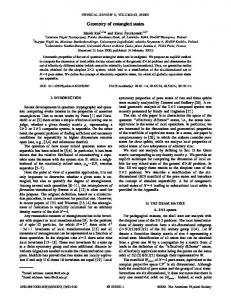
FIG. 1: (Color online) Schematic diagram of the top view of the device considered here. It consists of a rectangularshaped dc-SQUID and two mechanical resonators shown in blue on the left and right sides. These two opposite segments of the dc-SQUID are freely suspended and are treated as two nanomechanical resonators (NAMRs). The dotted lines indicate the equilibrium positions of the left and right NAMRs. Each “×”in the top segment of the loop represents a Josephson junction. XL (XR ) is the displacement of the center of the left (right) resonator. The two NAMRs could be located sufficiently “far apart” by using a SQUID with an appropriate aspect ratio. This could provide EPR-type correlations on the two NAMRs located sufficiently “far apart” for wide-enough SQUIDs.

We assume that the inductance of the dc-SQUID loop is negligibly small, and thus the magnetic energy of the circulating current in the dc-SQUID loop is neglected. Thus the voltage drop over the two junctions is zero. Therefore, ϕR − ϕL = ϕt , where ϕt is the phase related to total magnetic flux Φt threading the dc-SQUID loop ϕt = 2π

Φt . Φ0

(2)

Here Φ0 = h/2e is flux quantum. Introducing two new variables 1 (ϕR + ϕL ) , 2 1 = (ϕR − ϕL ) , 2

ϕ = ϕ−

(3a) (3b)

and taking into account that ϕ− = ϕt /2, the bias current in Eq. (1) can be written as Ib = 2Ic sin ϕ cos

between a dc-SQUID and two NAMRs is complicated and has many terms. However, if the frequency of the dc-SQUID is properly chosen by the bias current of the dc-SQUID, then only a few terms dominate the dynamics of the coupled system, which is illustrated by writing the interaction Hamiltonian in the interaction picture. Then, in Sec. III we study a special case where, under an appropriate choice of the parameters, the interaction Hamiltonian is simplified to study the two-mode parametric down-conversion process in the device. Squeezed states of the two NAMRs are studied by the HeisenbergLangevin method. Conclusions are given in Sec. IV.

(1)

ϕt . 2

(4)

It is here assumed that XL (XR ) is the amplitude for the fundamental flexural mode of the left (right) beam. Let BL (BR ) be the magnetic field normal to the plane of the SQUID loop near the left (right) mechanical beam and Φb the external applied magnetic flux threading perpendicularly the dc-SQUID loop when XL = XR = 0. It is assumed that BL (BR ) is constant in the oscillating region of the left (right) beam. Then, the total magnetic flux threading the dc-SQUID loop is given by Φ t = Φb + ΦX ,

(5)

where ΦX is the additional magnetic flux when the two NAMRs are displaced from their equilibrium positions: II.

COUPLING A DC-SQUID WITH TWO NANOMECHANICAL RESONATORS

The device we studied is schematically illustrated in Fig. 1. It consists of a dc-current-biased SQUID with rectangular shape and with two mechanical resonators. The left and right sides of the SQUID are suspended from the substrate and form the two mechanical oscillators, our NAMRs. We assume here that these two doubly-clamped beams vibrate in their fundamental flexural modes and in the plane of the SQUID loop. We use the following notations IL (IR ) for the current in the left (right) Josephson junction, and ϕL (ϕR ) for the phase drop in the left (right) Josephson junction. The two Josephson junctions are assumed to be identical and have the same critical current Ic . Thus the bias current

ΦX = BL XL l + BR XR l .

(6)

Here, l is the effective length of the left and right beam. l is defined as l ≡ SL /XL , where SL is the area between the equilibrium position of the NAMR and its bent configuration. Namely the area SL spans the region between the blue dashed line and the blue bent line in Fig. 1. Equation (6) indicates that the variables of the two NAMRs enter in the dynamics of the dc-SQUID by influencing the flux threading the dc-SQUID. The influence of the two NAMRs on the dynamics of the SQUID can also be revealed quantitatively in the potential energy of the dcSQUID, since this is also a function of the displacements of the two NAMRs. Thus, we first study the potential energy of the SQUID and afterwards the entire Hamiltonian of the coupled system.

3

U (M , ) X )

)X

(a)

(b)

(c) (c)

(d) (d)

M

FIG. 2: (Color online) The potential energy U (ϕ, ΦX ) (scaled by EJ ) of the dc-SQUID as a function of the phase variable ϕ and the magnetic flux ΦX originating from the displacements of the two NAMRs. The red color represents higher potential energy U , and the blue color represents lower potential energy. Both ϕ and ΦX are shown in units of π/Φ0 . In (a)-(c), the bias magnetic flux Φb threading the loop of the dc-SQUID is set at 2nΦ0 , (2n + 41 )Φ0 , and (2n + 21 )Φ0 , respectively; and the bias currents are all set at Ib = 0.1Ic . In (d), Φb = 2nΦ0 and Ib = 0.5Ic .

A.

monic oscillator. The charging energy of the dc-SQUID, Ec ≡ (2e)2 / (2CJ ), is assumed here to be much smaller than the modified Josephson energy (cos q0 )EJ of the dcSQUID. Here, q0 = sin−1 (Ib /2Ic ) is a value of ϕ which corresponds to one of the minima of the potential energy U (ϕ, ΦX ), when the two NAMRs are at their equilibrium positions. CJ is the capacitance of the left and right Josephson junctions. We then expand the potential U (ϕ, ΦX ) near one of its minimum points (ϕ, ΦX ) = (q0 , 0). When ΦX /Φ0 ≪ 1, and Φb = 2nΦ0 , the first cosine in Eq. (7) depends weakly on ΦX . Up to second order in ΦX , we can also expand After shifting the origin of ϕ to q0 , and omitting the constant terms, the potential energy in Eq. (7) becomes

Potential Energy of the Vibrating dc-SQUID

The potential energy of the dc-SQUID is U (ϕ, ΦX ) Φb Ib ΦX = −2EJ cos π cos ϕ − EJ ϕ , (7) +π Φ0 Φ0 Ic where EJ = ~Ic /(2e) is the Josephson energy of the junction31,32 . To have an idea of the situation under which the dc-SQUID can be described by a quasi-particle in a quadratic potential, in Fig. 2 (a)-(d) we plot this potential energy (7) for various values of the bias magnetic flux Φb and the bias current Ib . Since ΦX /Φ0 ≪ 1 in the case of experiments using a GHz NAMR, here we focus on the limit ΦX /Φ0 < 0.1 in Fig. 2. A particle in a quadratic potential can be described by a harmonic oscillator when its kinetic energy is much smaller than the barrier of the potential. We notice that, for the bias magnetic flux Φb = 2nΦ0 , with n being an integer, the phase variable ϕ falls in a potential well when the NAMRs oscillate around their equilibrium points. It is possible to approximate the dynamics of ϕ as a har-

U (ϕ, ΦX ) 2 ΦX = EJ (cos q0 ) ϕ2 − EJ (1 − cos q0 ) π Φ0 2 ΦX 1 2 π . (8) −EJ (sin q0 )ϕ + (cos q0 )ϕ 2 Φ0 Therefore, if the first term in the above potential is much larger than the other two terms, the dynamics of ϕ will still be well described by a harmonic oscillator. The higher order terms, such as π 4 Φ4X / 24Φ40 , in the expansion of cos (πΦX /Φ0 ) are negligibly small for the situation considered in our paper, when ΦX /Φ0 ≈ 10−3 . Theoretically, it is possible to increase the ratio πΦX /Φ0 by using a stronger magnetic field BL and BR and/or using soft NAMRs with greater zero-point fluctuations. However, in practice, the magnetic field is limited to (upmost) in tens Tesla and the zero-point fluctuations of the NAMRs is less than 10−12 m for the most of the experiments. Therefore, the periodic nature of the Josephson Hamiltonian has no chance to play a role here. Indeed the situation considered here is very similar to the optical parametric-down-conversion system, except for the coefficients of polynomial expansions of the interaction Hamiltonian. Now we consider how well a dc-SQUID is approximated by a harmonic oscillator. Since the barrier of the potential U (ϕ, ΦX ) has a finite height, the dynamics of ϕ is not an ideal harmonic oscillator. However, if the energy of the quasi-particle is small enough, the dynamics of ϕ can be approximately described by a harmonic oscillator. The maximum number Nmax of energy levels that can be confined in the potential U (ϕ, 0) is Nmax ≡ ∆U/Ω, where the height of the potential is ∆U = 2EJ [2 cos q0 + sin q0 (2q0 − π)] ,

(9)

and Ω is the frequency of the harmonic oscillator. B.

Hamiltonian of the Coupled System

Near the minimum potential U (q0 , 0), the free Hamiltonian of the dc-SQUID can be written as a harmonic

4 where

oscillator Hamiltonian Hs = Ec ϕ˙ 2 + EJ′ ϕ2 , ~

(10)

gL =

with

gR = EJ′ = EJ cos q0 ,

(11)

where the constant term has been omitted when we derived the Hamiltonian in Eq. (10). It is convenient to introduce the annihilation and creation operators a and a† : ′ 1/4 1/4 EJ Ec a = ϕ˙ , (12a) ϕ+i Ec EJ′ 1/4 ′ 1/4 Ec EJ † ϕ˙ . (12b) ϕ−i a = Ec EJ′ Then the free Hamiltonian in Eq. (10) of the dc-SQUID can be rewritten in the form Hs = ~Ω a† a , with the angular frequency q Ω = Ec EJ′ .

(13)

c2 =

(14)

Here, Xi and Pi are the coordinate and momentum operators of the ith NAMR; mi and ωi are the effective mass and angular frequency of the ith NAMR. The effective angular frequency ωi is not the one of the fundamental flexural mode, which is modified by the second term in the potential Eq. (8). Then the free Hamiltonian of the two NAMRs can be written in the form (16)

where the constant terms have been omitted. Thus, in terms of creation and annihilation operators, from Eq. (8), the interaction Hamiltonian between these two NAMRs and the dc-SQUID are given by h i2 V = − gL bL + b†L + gR bR + b†R h 2 i , (17) c1 a + a † + c2 a + a †

(18a) (18b) (18c) (18d)

The interaction Hamiltonian (17) is central to this work. Notice that it contains both linear and nonlinear terms. Generally, it is very difficult to evaluate the behavior of this coupled system. However, since the frequency Ω of the dc-SQUID can be set by the bias current Ib , we can reduce the interaction Hamiltonian V in Eq. (17) to a simplified form by invoking the rotating wave approximation. We now rewrite the interaction Hamiltonian V in Eq. (17) in the interaction picture, with the free Hamiltonian H0 = ~Ωa† a + ~ωL b†L bL + ~ωR b†R bR

When the energy of the dc-SQUID is not very large (ha† ai < Nmax ), the dynamics of ϕ is well described by a harmonic oscillator under a suitable bias magnetic flux threading the loop of the dc-SQUID. It is convenient to also introduce annihilation and creation operators for the fundamental flexural modes of the two NAMRs (i = L, R) r r mi ω i 1 Pi , (15a) Xi + i bi = 2~ 2~mi ωi r r mi ω i 1 † Pi . (15b) Xi − i bi = 2~ 2~mi ωi

HNAMR = ~ωL b†L bL + ~ωR b†R bR ,

c1 =

r πBL l ~ , Φ0 2mL ωL r πBR l ~ , Φ0 2mR ωR 1/4 Ω EJ cos q0 (tan q0 ) , 2 Ec Ω . 8

(19)

Then the terms of the interaction Hamiltonian V can be classified by the ways that the frequencies ωL , ωR , and Ω can be combined. In Table I, we list half of the coupling terms and the combinations of their frequencies. The other half are their corresponding Hermitian conjugate terms, which have the same frequencies but with a negative sign. In Table I, it can be seen that, for large detuning, one needs to mainly consider the zero-frequency terms in the first row of the table. Then this interaction Hamiltonian V enables a quantum nondemolition measurement of discrete Fock states of a NAMR, as discussed in Ref. 18. When the frequency of the dc-SQUID is set at some special value, one can mainly consider the resonant terms. For example, if the frequency of the dc-SQUID and those of the two NAMRs are properly set so that Ω 6= ωL = ωR and also Ω 6= 2ωL = 2ωR , then only the zero-frequency terms and resonant terms in the interaction Hamiltonian V are kept under the rotating wave approximation. The reduced interaction Hamiltonian Vr consists of the terms Vr = c2 gL gR b†R bL a† a + H.c. ,

(20)

which in fact offers us a mechanism for coupling two NAMRs. Thus, our proposed device offers a flexible (literately) model for the control and measurement of NAMRs. III.

TWO-MODE SQUEEZED STATES OF TWO NANOMECHANICAL RESONATORS

In this section we focus on the two-mode squeezed states of the two NAMRs. It is possible to produce

5

0 1 2 3 4 5 6 7 8 9 10 11 12 13 14 15 16 17 18 19 20 21 22

Frequencies 0 2ωL 2ωR ωL + ωR ωL − ωR 2Ω Ω 2ωL + 2Ω 2ωL − 2Ω 2ωR + 2Ω 2ωR − 2Ω ωL + ωR + 2Ω ωL + ωR − 2Ω ωL − ωR + 2Ω ωL − ωR − 2Ω 2ωL + Ω 2ωL − Ω 2ωR + Ω 2ωR − Ω ωL + ωR + Ω ωL + ωR − Ω ωL − ωR + Ω ωL − ωR − Ω

1 2

the device similarly to a light beam interacting inside a nonlinear medium in quantum optics, because both of them follow the same Hamiltonian (23). We now consider that the mode of the dc-SQUID is in a coherent state |αi, where |α| ≫ 1. Then we can treat the mode of the dc-SQUID as a classical field and replace the operator a in the Hamiltonian V ′ in Eq. (23) by a complex number |α| exp (−iφ). Then, in the interaction picture defined by the Hamiltonians (22) and (23), the dynamics of the coupled system is described by the following Hamiltonian

Interaction terms 2 † 2 † c2 (gL bL bL + g R bR bR )a† a, 2 2 † c2 gL bL a a, 2 2 † c2 gR bR a a, c2 gL gR bL bR a† a, c2 gL gR b†R bL a† a, 2 † 2 † c2 (gL bL bL + gR bR bR )a2 , 2 † 2 † c1 (gL bL bL + gR bR bR )a, 2 2 2 c2 gL bL a , 2 2 †2 c2 gL bL a , 2 2 2 c2 gR bR a , 2 2 †2 c2 gR bR a , c2 gL gR bL bR a2 , c2 gL gR bL bR a†2 , c2 gL gR bL b†R a2 , c2 gL gR bL b†R a†2 , 2 2 c1 gL bL a, 2 2 † c1 gL bL a , 2 2 c1 gR bR a, 2 2 † c1 gR bR a , c1 gL gR bL bR a, c1 gL gR bL bR a† , c1 gL gR bL b†R a, c1 gL gR bL b†R a† ,

VI = eiφ |α| η bL bR + e−iφ |α| η b†L b†R . The motions of bL and bR are bL (t) = cosh (γ) bL − ie−iφ sinh (γ) b†R ,

bR (t) = cosh (γ) bR − ie

sinh (γ) b†L

γ = |α| η t .

entangled states of the two NAMRs by considering the analog of the parametric down-conversion in quantum optics. The zero-frequency terms in Table I commute with the free Hamiltonian (13) of the dc-SQUID and the free Hamiltonian (16) of the two NAMRs. Let us assume that the proposed circuit works at low temperature. If the two NAMRs are initially in the vacuum state or in very low-energy states, then we have δLR ≪ Ω, with 2 2 δLR = c2 gR hb†R bR i + gL hb†L bL i . (21) Then we can rewrite the free Hamiltonians of the dcSQUID Eq. (13) and the two NAMRs Eq. (16) as (22)

where Ω′ = Ω−δLR . By properly setting the bias current Ib one can let Ω′ − ωL − ωR = 0. Then, in the interaction picture, after adopting the rotating wave approximation, we simplify the interaction Hamiltonian between two NAMRs and dc-SQUID as (23) V ′ = η a† bL bR + a b†L b†R , where η = −c1 gL gR .

−iφ

,

(26a) (26b)

in the interaction picture of the Hamiltonians (22) and (25), with

TABLE I: Terms in the interaction Hamiltonian Eq. (17) and their frequencies, in the interaction picture.

H0′ = Ω′ a† a + ωL b†L bL + ωR b†R bR ,

(25)

(24)

Driven by this interaction Hamiltonian V ′ , two-mode squeezed states of the two NAMRs can be produced in

(27)

The generation of two-mode squeezed states of these two NAMRs can be shown by their collective coordinate and momentum operators XT (t) = XL (t) + XR (t) , PT (t) = PL (t) + PR (t) ,

(28a) (28b)

where, Xi (t) and Pi (t), i = L, R, are defined by Eq. (15) by substituting bi and b†i with bi (t) and b†i (t) in Eq. (26). The uncertainty relation for the collective coordinate and momentum operators XT (t) and PT (t) is ∆ [XT (t)] ∆ [PT (t)] = ~ cosh2 γ + e2iφ sinh2 γ . (29) In Eq. (29) we have assumed that the zero-point fluctuation of positions of the left NAMR p δL = ~/(2mLωL ), (30)

and that of the right NAMR p δR = ~/(2mR ωR )

(31)

are the same. Here

δX =

√

2δL =

√

2δR

(32)

is defined as the zero-point fluctuation of the collective coordinates XT of the two NAMRs. And ζP = √ √ 2ζL = 2ζR is defined as the zero-point fluctuation of the collective momentums PT of the two NAMRs. Here, ζi2 = ~/(2δi2 ), i = L, R. If we choose φ = −π/2, then the variance of the collective coordinates XT (t) becomes ∆ [XT (t)] = δX exp(γ) .

(33)

6 Notice that γ < 0 because γ = −c1 gL gR |α| t. Therefore, perfect two-mode squeezed states, i.e., pure entangled states, of the two NAMRs are generated. The variance of XT (t) (the entanglement) was obtained above by assuming that both the left and right NAMRs be in their ground states. It can be checked that if both the left and right NAMRs are initially in coherent states or thermal states, then the Hamiltonian (25) will not produce entangled states of them. However, if only one of the NAMRs is initially prepared into a number state, then entangled states of these two NAMRs can be generated by the Hamiltonian (25). For example, when the left and the right NAMRs are initially prepared in the number states |0i and |1i, respectively, then the Bell-type entangled state a1 |01i + a2 |10i can be generated. Here, a1 and a2 are complex numbers. When one of the two NAMRs is initially in a coherent state and the other one is in the vacuum state, then the so-called “single-photonadded coherent states”33 can be generated by the Hamiltonian (25). Let us now consider the more realistic case where both the dc-SQUID and the two NAMRs are coupled to their environments. The quality factors of the two NAMRs with GHz frequency are smaller than that of the dcSQUID6,34 . The quality factor of a GHz NAMR is of the order of 103 , while that of a superconducting circuit can be as large as 106 . Therefore, below we consider the noise from the environment acting on the two NAMRs. To include damping effects, due to the noise from the environments, on the dynamics of the two NAMRs, we use the Heisenberg-Langevin equation method35 . Then, for the motions of the operators of the NAMRs, we have the following set of equations: d κL bL = −ξb†R − bL + FL (t) , dt 2 κR d bR = −ξb†L − bR + FR (t) , dt 2

(34a) (34b)

As in the ideal case in Eq. (33) we also let φ = −π/2. Here, ξ = |α| η

(35)

is the effective coupling strength between the dc-SQUID and two NAMRs. Also, κL and κR represent the damping rates of the left and right NAMRs, respectively; and the associated noise operators are FL (t) and FR (t). We evaluate the properties of the states of the two NAMRs by the variance of the collective coordinates XT . We find that the damping of the two NAMRs help producing twomode squeezed states of the two NAMRs, regardless of the initial states. The variance of the collective coordinates XT is calculated as [∆ (XT )]2 =

2 δL δ2 (2κR ∆ξ + κ− ) + R (2κL ∆ξ − κ− ) κ+ κ+ δL δR ξ ∆ξ , (36) −8 κ+

1

G X2

30

0.25 0

20 10

NR /[

10

20

NL /[

30 0

FIG. 3: (Color online) The squared variance of the collective coordinates XT of the two NAMRs as the function of damping rates κL and κR of the left and right NAMRs, both κL and κR are normalized by the effective coupling constant ξ. Here, δX is the zero fluctuation of the collective coordinates of the two NAMRs.

under the Markov approximation and in the overdamped case: ξ < κL /2 and ξ < κR /2. In the Appendix A we outline the main ideas of the derivation. Here, κ± = κL ± κR , ∆ξ =

κL κR . κL κR − 4ξ 2

(37)

When the zero-point fluctuations of the left and right NAMRs are equal, we have 2 4ξ δX 2 . (38) [∆ (XT )] = ∆ξ 1 − 4 κL + κR Fig. 3 shows, the variance of the collective coordinates XT versus the damping rates κL and κR . It is clear from Fig. 3 that appreciable squeezing can be generated even when the dampings of the two NAMRs are severe (ten times the coupling constant ξ). This indicates that the squeezing is robust against damping. The maximum squeezing is obtained when both damping rates (for the left and right NAMRs) approach the coupling strength between them and the dc-SQUID. Since the coupling strength ξ is proportion to |α|, one can increase the squeezing rate by gradually increasing the power of the microwave applied to the dc-SQUID. As the damping rates of the two NAMRs increase, the squeezing effect decreases steadily. To consider the experimental feasibility of our proposal, we choose the following parameters for the two NAMRs and the dc-SQUID mL ωL ωR l BL κL EC EJ

= = = = = = = =

mR = 10−18 Kg, 1.5 GHz, 1.2 GHz, 10 µm, BR = 1 T, κR = 2 MHz, 0.061 GHz, 120 GHz.

(39a) (39b) (39c) (39d) (39e) (39f) (39g) (39h)

7 It was already demonstrated in experiments6,36 that a 10 µm long doubly-clamped beam can oscillate with a frequency of several Giga Hertzs. The effective mass of this antenna-shaped beam is much smaller than its weight. And its effective mass can be further modified when the beams are under strains and stresses. The numbers used here for the dc-SQUID are also consistent with the experimental numbers shown in Ref. 37. Then the additional magnetic flux from the two NAMRs, ΦX /Φ0 ≃ 5 × 10−3 ≪ 1, would satisfy our assumption in section II. The maximum number Nmax of energy levels confined in the current biased potential energy is calculated as Nmax ≃ 150. Therefore, the harmonic oscillator approximation and the classical field approximation for the dc-SQUID are both possible. The time needed to obtain the two-mode squeezed state is determined by the effective coupling constant ξ. Assuming the same damping rates for the two NAMRs, the maximum squeezing ∆ (XT ) = (1/2) δX can be obtained. Therefore, it should be possible to realize our proposal of generating twomode squeezed states of the two NAMRs with current experimental conditions. To experimentally detect the generated two-mode squeezed state of the two NAMRs, a (in principle) relatively direct method would be checking the variance of the collective coordinate XT of the two NAMRs. Since the left and right NAMRs are symmetric in the interaction Hamiltonian (17), they can be treated as one virtual NAMR. To detect two-mode squeezed states of the two NAMRs, the detection methods should be able to approach standard quantum limit of the NAMRs. With traditional displacement detection methods1,4,39,40,41 , such as optical interferences, magnetic-motive method and coupled single electron transistor, the best record of detection precision was about 4.3 standard quantum limits38 . There are also other proposals for displacement detection by coupling the mechanical oscillator to some two level system13,19,21 . These methods in principle can detect quantum states of the NAMRs. After the entangled state is generated, one can switch the dc-SQUID to the phase qubit regime42 , and utilize the nonlinear coupling between the virtual NAMR and the dc-SQUID. Then the SQUID can be used to measure the variance of XT , as discussed in Ref. 21.

IV.

netic flux through the dc-SQUID, thereby these modes cannot be coupled to the dc-SQUID, even through their frequencies match the resonant condition. It is similar to the case of the experiments of magnetomotive detection of flexural oscillation of NAMRs1 , where torsional and strain-stress oscillations have been neglected. As mentioned in Section. III, to generate two-mode squeezed states of NAMRs, the NAMRs should start in their ground states or number states. The NAMRs should be cooled such that the thermal excitation energy is less than those corresponding to the NAMRs’ frequencies. For a one-GHz NAMR, this means that the temperature should be below 50 mK, which is still within the capability of dilution refrigerators. In principle it is possible to prepare the NAMRs used in our proposal in their ground states. Moreover, recently there have been many efforts in reducing the temperature of mechanical resonators by active cooling43,44,45,46,47 . Also a temperature as low as 5 mK was already demonstrated for a mechanical resonator47. Besides, there are also theoretical proposals for the production of number states of NMARs48 . Therefore, though currently the ground states and (or) number states of NAMRs might be difficult to prepare experimentally, we expect these to be realized more earlier in the near future. For example, if the temperature of a GHz NAMR reaches 10 mk, the thermal occupation number will be ∼ 10−3 , which is nearly a ground state. In conclusion, we have proposed a device to couple a dc-SQUID to two NAMRs, which can be used to create an effective coupling between these two NAMRs, and also to measure and control the two NAMRs. We have shown that two-mode squeezed states can be generated in a robust fashion by this device, in analogy to the two-mode parametric down-conversion process in quantum optics. This two-mode down-conversion process offers us a protocol of producing entanglement in two mechanical resonators in a solid state device, while previous proposals, see, e.g., Refs. 24,25,49, were based on entanglementswapping by the assistance of photons. Our proposal might be promising for the experimental test of the existence of entangled states of macroscopic objects.

DISCUSSIONS AND CONCLUSIONS V.

In our proposal, we only consider the fundamental vibration modes of the NAMRs. Generally, there are also vibration modes with higher frequencies, torsional and strain-stress oscillations in the NAMRs1 . The vibration modes with higher frequencies will be excited only when they happen to resonate with the dc-SQUID, which can be easily avoided by optimizing the parameters of the NAMRs. As for torsional and strain-stress oscillations, they are hardly coupled to the dc-SQUID. These modes of oscillations of the NAMRs will not change the mag-

ACKNOWLEDGEMENT

FN was supported in part by the US National Security Agency (NSA), Army Research Office (ARO), Laboratory of Physical Sciences (LPS), and the National Science Foundation grant No. EIA-0130383. CPS was supported in part by the NSFC with grant Nos. 90203018, 10474104 and 60433050; and the National Fundamental Research Program of China with Nos. 2001CB309310 and 2005CB724508.

8 APPENDIX A: HEISENBERG-LANGEVIN EQUATION FOR TWO NANOMECHANICAL RESONATORS

D We Econsider the Markov approximation hFL,R i = † FL,R = 0. Using Eqs. (34a)-(34b), a solution of the

expectation values hbL (t)i and hbR (t)i can be given as h i 1 hbL i = e− 2 κL t bL (0) cosh (ξt) − b†R (0) sinh (ξt) , hbR i = e

− 12 κR t

(A1a) h i † bR (0) cosh (ξt) − bL (0) sinh (ξt) .

represents the transpose operation. Here 

B (t) = e−Mt B (0) +

The variance of the collective coordinates XT can be evaluated by the expectation values of the bilinear operators of the two NAMRs. These are the expectation values of the quadratic operators of the left NAMR D E

, (A3a) L1 = b2L , L3 = b†2 L E D (A3b) L2 = b†L bL + bL b†L , the expectation values of the quadratic operators of the right NAMR D E

, (A4a) R1 = b2R , R3 = b†2 R E D (A4b) R2 = b†R bR + bR b†R , and the expectation values of the quadratic operators of both NAMRs C4†

C1 = hbL bR + bR bL i = , D E † † † C2 = bL bR + bR bL = C3 .

From Eq. (34) it is found that these expectation values satisfy a closed set of equations of motion35 . To determine the values involving the expectation values of the products of the noise operators and the operators of the NAMRs, we rewrite Eq. (34a)-(34b) and their corresponding Hermitian ones in the matrix form B˙ = −MB + F ,

(A6)

iT h where B = bL (t) , b†L (t) , bR (t) , b†R (t) and F = iT h T FL (t) , FL† (t) , FR (t) , FR† (t) are vectors, and [...]

 ξ 0  . 0 

Z

0

t

e−M(t−t ) F (t′ ) dt′ . ′

B (t) F † (t) = e−Mt B (0) F † (t) Z t ′ e−M(t−t ) F (t′ ) dt′ F † (t) . +

(A7)

(A8)

(A9)

0

Since the operators of the NAMRs at the initial time t = 0 are statistically independent of the noise opera

tors, we have B (0) F † (t) = 0. Using the fact that the corresponding elements of the matrix of the left part of Eq. (A9) and those of the matrix of the right part of Eq. (A9) are equal, and combining the Markov approximation, we obtain E D κL bL (t) FL† (t) = , (A10a) 2 D E κR bR (t) FR† (t) = . (A10b) 2 All other products of the operators of the two NAMRs and the noise operators are zero. Therefore, in the interaction picture, finally when the expectation values of these bilinear operators do not change with time, the solution of the above set of equations reads L1 = L3 = R1 = R3 = C2 = C3 = 0 ,

(A11)

and

(A5a) (A5b)

0 ξ

Multiplying the above equation by F † (t) from the right side, we obtain

It is seen that below the thresholds ξ < κL /2 and ξ < κR /2 we have (A2)

0

κL 2

 0 M = 0 ξ κ2R ξ 0 0 κ2R A formal solution of Eq. (A6) is given by

(A1b)

hbL i = hbR i = 0 .

κL 2

κ− 2κR + ∆ξ , κ+ κ+ κ− 2κL + ∆ξ , = − κ+ κ+ 4ξ = C4 = − ∆ξ . κ+

L2 =

(A12a)

R2

(A12b)

C1

(A12c)

with ξ < κL /2 and ξ < κR /2. Also, in the interaction picture, we have hbL (t)i = hbR (t)i = 0 after a sufficiently long time. Therefore, the variance of the collective coordinate XT becomes 2 2 [∆ (XT )]2 = δL L 2 + δR R2 + δL δR (C1 + C4 )

This provides the main result of section III.

(A13)

9

1

2

3 4

5

6

7

8

9

10 11 12

13

14

15

16

17

18

19

20

21 22

23

24

25

A. N. Cleland, Foundations of nanomechanics: From Solid-State Theory to Device Applications (SpringerVerlag, Berlin, 2002). R. H. Blick, A. Erbe, L. Pescini, A. Kraus, D. V. Scheible, F. W. Beil, E. Hoehberger, A. Hoerner, J. Kirschbaum, H. Lorenz, et al., J. of Phys.: Cond. Mat. 14, R905 (2002). M. Blencowe, Phys. Rep. 395, 159 (2004). K. Schwab and M. Roukes, Physics Today 58 (6), 36 (2005). X. M. H. Huang, C. A. Zorman, M. Mehregany, and M. L. Roukes, Nature 421, 496 (2003). A. Gaidarzhy, G. Zolfagharkhani, R. L. Badzey, and P. Mohanty, Phys. Rev. Lett. 94, 030402 (2005). K. C. Schwab, M. P. Blencowe, M. L. Roukes, A. N. Cleland, S. M. Girvin, G. J. Milburn, and K. L. Ekinci, Phys. Rev. Lett. 95, 248901 (2005). A. Gaidarzhy, G. Zolfagharkhani, R. L. Badzey, and P. Mohanty, Phys. Rev. Lett. 95, 248902 (2005). S. Savel’ev, X. Hu, and F. Nori, New J. of Phys. 8, 105 (2006); cond-mat/0601019. S. Savel’ev and F. Nori, Phys. Rev. B 70, 214415 (2004). N. Nishiguchi, Phys. Rev. B 68, 121305(R) (2003). S. Savel’ev, A. L. Rakhmanov, X. Hu, A. Kasumov, and F. Nori, Phys. Rev. B 75, 165417 (2007). A. D. Armour, M. P. Blencowe, and K. C. Schwab, Phys. Rev. Lett. 88, 148301 (2002). Y. D. Wang, Y. B. Gao, and C. P. Sun, Eur. Phys. J. B 40, 321 (2004). P. Zhang, Y. D. Wang, and C. P. Sun, Phys. Rev. Lett. 95, 097204 (2005). C. P. Sun, L. F. Wei, Y.-X. Liu, and F. Nori, Phys. Rev. A 73, 022318 (2006). L. F. Wei, Y.-X. Liu, C. P. Sun, and F. Nori, Phys. Rev. Lett. 97, 237201 (2006). E. Buks, E. Arbel-Segev, S. Zaitsev, B. Abdo, and M. P. Blencowe, quant-ph/0610158 (2006). F. Xue, Y. D. Wang, C. P. Sun, H. Okamoto, H. Yamaguchi, and K. Semba, New Journal of Physics 9, 35 (2007). F. Xue, L. Zhong, Y. Li, and C. P. Sun, Phys. Rev. B 75, 033407 (2007). X. Zhou and A. Mizel, Phys. Rev. Lett. 97, 267201 (2006). P. Rabl, A. Shnirman, and P. Zoller, Phys. Rev. B 70, 205304 (2004). R. Ruskov, K. Schwab, and A. N. Korotkov, Phys. Rev. B 71, 235407 (2005). S. Mancini, V. Giovannetti, D. Vitali, and P. Tombesi, Phys. Rev. Lett. 88, 120401 (2002). S. Pirandola, D. Vitali, P. Tombesi, and S. Lloyd, Phys. Rev. Lett. 97, 150403 (2006).

26

27 28 29 30 31 32 33

34

35

36

37

38

39

40

41

42

43

44

45

46

47

48

49

J. Eisert, M. B. Plenio, S. Bose, and J. Hartley, Phys. Rev. Lett. 93, 190402 (2004). X. Hu and F. Nori, Phys. Rev. Lett. 76, 2294 (1996). X. Hu and F. Nori, Phys. Rev. B 53, 2419 (1996). X. Hu and F. Nori, Phys. Rev. Lett. 79, 4605 (1997). X. Hu and F. Nori, Physica B 263, 16 (1999). J. Q. You and F. Nori, Physics Today 58 (11), 42 (2005). G. Wendin and V. Shumeiko, cond-mat/0508729 (2005). A. Zavatta, S. Viciani, and M. Bellini, Science 306, 660 (2004). P. K. Day, H. G. LeDuc, B. A. Mazin, A. Vayonakis, and J. Zmuidzinas, Nature 425, 817 (2003). M. O. Scully and M. S. Zubairy, Quantum Optics (Cambridge University Press, Cambridge, 1997). A. Gaidarzhy, G. Zolfagharkhani, R. L. Badzey, and P. Mohanty, App. Phys. Lett. 86, 254103 (2005). S. O. Valenzuela, W. D. Oliver, D. M. Berns, K. K. Berggren, L. S. Levitov, and T. P. Orlando, Science 314, 1589 (2006). M. D. LaHaye, O. Buu, B. Camarota, and K. C. Schwab, Science 304, 74 (2004). J. N. Munday, D. Iannuzzi, Y. Barash, and F. Capasso, Phys. Rev. A. 71, 042102 (2005). J. N. Munday, D. Iannuzzi, and F. Capasso, New J. of Phys. 8, 244 (2006). F. Capasso, J. N. Munday, D. Iannuzzi, and H. B. Chan, IEEE J. of Selected Topics in Quantum Electronics 13, 400 (2007). K. B. Cooper, M. Steffen, R. McDermott, R. W. Simmonds, S. Oh, D. A. Hite, D. P. Pappas, and J. M. Martinis, Phys. Rev. Lett. 93, 180401 (2004). A. Naik, O. Buu, M. D. LaHaye, A. D. Armour, A. A. Clerk, M. P. Blencowe, and K. C. Schwab, Nature 443, 193 (2006). A. Schliesser, P. Del’Haye, N. Nooshi, K. J. Vahala, and T. J. Kippenberg, Phys. Rev. Lett. 97, 243905 (2006). D. Kleckner and D. Bouwmeester, Nature (London) 444, 75 (2006). S. Gigan, H. R. Bohm, M. Paternostro, F. Blaser, G. Langer, J. B. Hertzberg, K. C. Schwab, D. Bauerle, M. Aspelmeyer, and A. Zeilinger, Nature (London) 444, 67 (2006). M. Poggio, C. L. Degen, H. J. Mamin, and D. Rugar, condmat/0702446 (2007). E. K. Irish and K. C. Schwab, Phys. Rev. B 68, 155311 (2003). J. Zhang, K. Peng, and S. L. Braunstein, Phys. Rev. A 68, 013808 (2003).