May 14, 2009 - ... the ground and first excited vibrational states, âNj = N0,j â N1,j. ...... [ 99 ] Ayotte, P., S. B. Nielsen, G. H. Weddle, M. A. Johnson, and S. S. Xanth- ... [ 108 ] Asbury, J. B., T. Steinel, K. Kwak, S. A. Corcelli, C. P. Lawrence, J. L. ...
Ultrafast Spectroscopy of Model Biological Membranes
Ultrafast Spectroscopy of Model Biological Membranes
Proefschrift ter verkrijging van de graad van Doctor aan de Universiteit Leiden, op gezag van de Rector Magnificus, Prof. Mr. Dr. Paul F. van der Heijden, volgens besluit van het College voor Promoties in het openbaar te verdedigen op Woensdag 2 September 2009 klokke 13.45 uur
door
Avishek Ghosh geboren op 20 Augustus 1979 te London, U.K.
Promotiecommissie Promotor:
Prof. Dr. Mischa Bonn
Overige leden:
Prof. Dr. Aart Kleyn Prof. Dr. Huib J Bakker Prof. Dr. Marc Koper Dr. Jens Bredenbeck Dr. Sander Woutersen Prof. Dr. Jaap Brouwer Prof. Dr. Geert-Jan Kroes Prof. dr. Marc C. van Hemert
This thesis is based on the following publications: 1. Avishek Ghosh, Marc Smits, Jens Bredenbeck, Niels Dijkhuizen and Mischa Bonn. Femtosecond time-resolved and 2D vibrational sum frequency spectroscopy to study structural dynamics at interfaces. Rev. Sci. Instrum. 79, 093907 (2008) 2. Marc Smits∗ , Avishek Ghosh∗ , Martin Sterrer, Michiel Muller, Mischa Bonn. Ultrafast Vibrational Energy Transfer between Surface and Bulk Water at the Air-Water Interface. Phys. Rev. Lett. 98, 098302 (2007) 3. Avishek Ghosh, Marc Smits, Jens Bredenbeck, Mischa Bonn. Membrane-bound water is energetically decoupled from nearby bulk water: An ultrafast surfacespecific investigation. J. Am. Chem. Soc. 129, (31), 9608-9609 (2007) 4. Avishek Ghosh, Marc Smits, Maria Sovago, Jens Bredenbeck, Michiel Muller, Mischa Bonn. Ultrafast vibrational dynamics of interfacial water. Chem. Phys. 350, (1-3), 23-30 (2008) 5. Avishek Ghosh, Maria Sovago, R. Kramer Campen and Mischa Bonn. Structure and dynamics of interfacial water in model lung surfactants. Faraday Discuss. 141, 1-15 (2008) 6. Marc Smits∗ , Avishek Ghosh∗ , Jens Bredenbeck, Susumu Yamamoto, Michiel Mller and Mischa Bonn. Ultrafast energy flow in model biological membranes. New J. Phys. 9, 390 (2007) 7. Avishek Ghosh, R.K. Campen and Mischa Bonn. Ultrafast vibrational dynamics of water at various lipid-water interfaces. (in preparation) Other Publications: • Jens Bredenbeck, Avishek Ghosh, Marc Smits, Mischa Bonn. Ultrafast Two Dimensional-Infrared Spectroscopy of a Molecular Monolayer. J. Am. Chem. Soc. 130 (7), 2152-2153 (2008) • Jens Bredenbeck, Avishek Ghosh, Marc Smits, Han-Kwang Nienhuys and Mischa Bonn. Interface-Specific Ultrafast Two-Dimensional Vibrational Spectroscopy. Acc. Chem. Res. (in press) (Web published: May 14, 2009).
∗
contributed equally to this work
Contents
Chapter 1 Introduction 1.1 Interfaces - A General Perspective . . . . . . . . . . . . . . . . . . . . . . . 1.2 Interfaces in Biology . . . . . . . . . . . . . . . . . . . . . . . . . . . . . . . 1.3 Membranes and Interfacial Water . . . . . . . . . . . . . . . . . . . . . . . . 1.4 Challenges in probing interfacial water . . . . . . . . . . . . . . . . . . . . . 1.5 Vibrational Sum Frequency Generation (VSFG) Spectroscopy - The Surface 1.5.1 Concepts in Nonlinear Polarization . . . . . . . . . . . . . . . . . . . 1.5.2 Sum Frequency Generation . . . . . . . . . . . . . . . . . . . . . . . 1.5.3 Vibrational Sum Frequency Generation at Interfaces . . . . . . . . . 1.5.3.1 Properties of χ(2) and surface-sensitivity of VSFG . . . . . 1.5.3.2 VSFG - A surface-specific IR probe . . . . . . . . . . . . . 1.6 Time-Resolved SFG Spectroscopy . . . . . . . . . . . . . . . . . . . . . . . . 1.7 Thesis Outline . . . . . . . . . . . . . . . . . . . . . . . . . . . . . . . . . .
. . . . . . . . . . . . . . . . Probe . . . . . . . . . . . . . . . . . . . . . . . . . . . .
. . . . . . . . . . . .
1 1 3 4 6 7 7 8 9 11 12 13 15
Chapter 2 Experimental Technique 2.1 Introduction . . . . . . . . . . . . . . . . . . . . . . . . . . . . . . 2.2 Generation of Mid-IR and Visible upconversion pulses for VSFG 2.3 Instrumentation at Sample . . . . . . . . . . . . . . . . . . . . . 2.4 Detection Schemes and Data Acquisition . . . . . . . . . . . . . . 2.5 Software and Electronics . . . . . . . . . . . . . . . . . . . . . . . 2.6 Getting Started . . . . . . . . . . . . . . . . . . . . . . . . . . . .
. . . . . .
. . . . . .
16 17 17 23 24 27 29
Chapter 3 Ultrafast Energy Transfer between Interfacial and Bulk Water at the Air-Water Interface 3.1 Introduction . . . . . . . . . . . . . . . . . . . . . . . . . . . . . . . . . . . . . . . . . 3.2 Static and Time-resolved VSFG experiments . . . . . . . . . . . . . . . . . . . . . . 3.3 Results and Discussion . . . . . . . . . . . . . . . . . . . . . . . . . . . . . . . . . . . 3.3.1 Static SFG Results . . . . . . . . . . . . . . . . . . . . . . . . . . . . . . . . . 3.3.2 Time-resolved SFG Results . . . . . . . . . . . . . . . . . . . . . . . . . . . . 3.4 Conclusions . . . . . . . . . . . . . . . . . . . . . . . . . . . . . . . . . . . . . . . . .
31 32 33 36 36 37 42
. . . . . .
. . . . . .
. . . . . .
. . . . . .
. . . . . .
. . . . . .
. . . . . .
. . . . . .
. . . . . .
Chapter 4 Ultrafast Dynamics of Water at various lipid-water interfaces 4.1 Introduction . . . . . . . . . . . . . . . . . . . . . . . . . . . . . . . . . . . . . . . . . 4.2 Surface-specific Vibrational Spectroscopy: Frequency- and Time-Resolved Sum Frequency Generation . . . . . . . . . . . . . . . . . . . . . . . . . . . . . . . . . . . . .
43 44 44
Contents 4.3 4.4
4.5
Experimental Section . . . . . . . . . . . . . . Results and Discussion . . . . . . . . . . . . . 4.4.1 Frequency-resolved SFG experiments . 4.4.2 Time-resolved SFG experiments . . . 4.4.2.1 DPTAP/H2 O Interface . . . 4.4.2.2 DMPS/H2 O Interface . . . . 4.4.2.3 DPPC/H2 O and DPPE/H2 O Conclusion . . . . . . . . . . . . . . . . . . .
. . . . . . . . . . . . . . . . . . . . . . . . . . . . . . . . . . . . Interface . . . . . .
. . . . . . . .
. . . . . . . .
. . . . . . . .
. . . . . . . .
. . . . . . . .
. . . . . . . .
. . . . . . . .
. . . . . . . .
. . . . . . . .
. . . . . . . .
. . . . . . . .
. . . . . . . .
. . . . . . . .
. . . . . . . .
. . . . . . . .
. . . . . . . .
46 47 47 49 51 54 55 59
Chapter 5 Structure and Dynamics of Water at Model Human Lung Surfactant interfaces 61 5.1 Introduction . . . . . . . . . . . . . . . . . . . . . . . . . . . . . . . . . . . . . . . . . 62 5.1.1 Lung Surfactants and Interfacial Water . . . . . . . . . . . . . . . . . . . . . 62 5.1.2 Frequency- and Time-Resolved SFG on model lung surfactant monolayers on water . . . . . . . . . . . . . . . . . . . . . . . . . . . . . . . . . . . . . . . . 63 5.2 Results and Analysis . . . . . . . . . . . . . . . . . . . . . . . . . . . . . . . . . . . . 65 5.2.1 Frequency-resolved VSFG measurements . . . . . . . . . . . . . . . . . . . . . 65 5.2.2 Time-resolved SFG measurements . . . . . . . . . . . . . . . . . . . . . . . . 67 5.3 Discussion . . . . . . . . . . . . . . . . . . . . . . . . . . . . . . . . . . . . . . . . . . 70 5.3.1 Frequency-resolved SFG measurements . . . . . . . . . . . . . . . . . . . . . . 70 5.3.2 Time-resolved SFG measurements . . . . . . . . . . . . . . . . . . . . . . . . 70 5.4 Conclusions . . . . . . . . . . . . . . . . . . . . . . . . . . . . . . . . . . . . . . . . . 72 Chapter 6 Ultrafast energy flow in model biological membranes 6.1 Introduction . . . . . . . . . . . . . . . . . . . . . . . . . 6.2 Time-resolved Surface Spectroscopy . . . . . . . . . . . 6.2.1 Steady-state Sum Frequency Generation . . . . . 6.2.2 Time-resolved Sum Frequency Generation . . . . 6.3 Experiment . . . . . . . . . . . . . . . . . . . . . . . . . 6.3.1 Sample preparation . . . . . . . . . . . . . . . . 6.4 Results . . . . . . . . . . . . . . . . . . . . . . . . . . . . 6.4.1 Static SFG Spectra . . . . . . . . . . . . . . . . . 6.4.2 Time Resolved SFG Spectra . . . . . . . . . . . . 6.4.2.1 DPPC . . . . . . . . . . . . . . . . . . . 6.4.2.2 DOPC . . . . . . . . . . . . . . . . . . 6.4.2.3 Heat transfer across the monolayer . . . 6.4.3 Data Analysis . . . . . . . . . . . . . . . . . . . . 6.5 Discussion . . . . . . . . . . . . . . . . . . . . . . . . . . 6.6 Conclusions and Outlook . . . . . . . . . . . . . . . . . Bibliography
. . . . . . . . . . . . . . .
. . . . . . . . . . . . . . .
. . . . . . . . . . . . . . .
. . . . . . . . . . . . . . .
. . . . . . . . . . . . . . .
. . . . . . . . . . . . . . .
. . . . . . . . . . . . . . .
. . . . . . . . . . . . . . .
. . . . . . . . . . . . . . .
. . . . . . . . . . . . . . .
. . . . . . . . . . . . . . .
. . . . . . . . . . . . . . .
. . . . . . . . . . . . . . .
. . . . . . . . . . . . . . .
. . . . . . . . . . . . . . .
. . . . . . . . . . . . . . .
74 75 77 77 78 79 79 80 80 82 83 85 85 87 89 90 91
Summary
104
Samenvatting
108
Dankwoord
112
Curriculum Vitae
114
Chapter
1
Introduction 1.1
Interfaces - A General Perspective
Surfaces are ubiquitous in nature. Essentially, of everything we see around us, we observe the exposed surface. Surfaces define the boundary with the surrounding environment and influence interactions with that environment, and so it is no surprise that surfaces and interfaces have been intensely studied. We are confronted with interfaces almost every day through phenomena like corrosion, tarnishing of metals, friction, lubrication of moving parts,adhesives, surface tension in liquids and a variety of heterogeneous chemistry in atmospheric (e.g., aerosol chemistry), geological (e.g., mineral oxide-water interfaces) and biological processes. The discipline ’Surface Science’ deals with surfaces ranging from very well-defined single-crystal metal surfaces in ultra high vacuum to extremely complex surfaces of biological cells in living organisms. These efforts are prompted both by a fundamental interest in these intriguing systems, and by the technological importance of surfaces and interfaces: industrial-scale heterogeneous catalysis - whereby reactants (monomers) are adsorbed typically on a metallic surface which reduces the activation energy barrier and provides the essential reaction site - has revolutionized the polymer, petroleum, food and automobile industries today; large surface area materials have been essential for this development. Asymmetric heterogeneous catalysis has recently been used to synthesize enantiomerically pure compounds using chiral heterogeneous catalysts; implications of this development in drug discovery and medicinal chemistry can only be imagined. Metal-insulator interfaces are beginning to show their true power in emerging technologies, like spintronics - whereby the intrinsic electron spins can be used to transport information efficiently. For instance, a major breakthrough has recently been reported on transporting electron spins by efficient quantum-mechanical tunneling through a thin layer of insulator, interfacial with two flanking ferromagnetic layers - termed as Tunnel Magneto-Resistance [1]]. So we see interfaces of different materials have remarkable properties that can truly revolutionize existing, and emerging technologies likewise. Arguably one of the most important interfaces is the membrane surrounding living cells, which enclose a small volume of aqueous solution and separate it from the outside. However, membranes are not simply passive molecular barriers between the interior and the exterior; in fact, their active participation in a variety of natural phenomena is essential for life. In this thesis, we aim at getting
new insights into biological membranes using novel laser-based techniques. There is a major challenge associated with obtaining a comprehensive understanding of the complex physics and chemistry of interfaces, owing to the difficulty in probing a few angstroms of matter. Nobel Laureate Wolfgang Pauli once said, God made the bulk; the surface was invented by the devil. Pauli explained that the diabolical properties of surfaces were due to the simple fact that surface atoms do not have an isotropic environment: they interact with three different types of atoms: those in the bulk below, other atoms from the same surface, and atoms in the adjacent phase. As a result, the properties of surface atoms are very different from those in the adjacent bulk media. With intense experimental pursuits and the advent of a wide variety of surface techniques over the past 50 years, like transmission electron microscopy [2, 3]], low energy electron diffraction [4, 5]], scanning tunneling microscopy [6–8]], atomic force microscopy [6, 9]], neutron reflectometry [10]], neutron scattering [11]] and X-ray diffraction [12,13]], complemented by powerful molecular dynamics simulation studies [14–20]], our understanding of surfaces has been radically enhanced, as testified by a variety of emergent surface technologies and a better control over the variety of fundamental interfacial phenomena observed in nature. The applicability of many surface science techniques is limited to surface samples that can withstand ultrahigh vacuum (UHV) conditions. These techniques are often invasive and generally set specific requirements on the samples, that limit the types of interfaces that can be studied. For instance, UHV conditions are not conducive to study solid-liquid and liquid-liquid interfaces. Probing surfaces by optical techniques is, in general, more flexible, non-invasive and is applicable to samples in their native environment. Indeed, optical techniques such as surface plasmon resonance [21, 22]] and reflection absorption IR spectroscopy [23–25]] have been insightful while probing surfaces noninvasively. In the past two decades, second-order nonlinear optical techniques of second harmonic generation (SHG) and sum frequency generation [26–30]] (SFG) have proven to be versatile noninvasive tools for probing all kinds of interfaces with excellent molecular and surface specificities. The strength of these techniques for studying surfaces and interfaces lies in their inherent surface specificity. Although it was established in the mid-sixties that second harmonic and sum frequency generation could be used to investigate specifically the structures of surfaces and interfaces of centrosymmetric materials (under the electric dipole approximation), it was not until about 1980 that technical advances in laser sources enabled nonlinear optical spectroscopy of surfaces to become well established as a separate subfield1 In this thesis I present briefly, the vibrationally-resonant sum frequency generation (VSFG) technique that we use to to probe molecular processes at liquid-vapor interfaces but primarily introduce a novel time-resolved IR pump - VSFG technique in our continuing quest to unravel some of the mysterious dynamical phenomena associated with biological membranes.
1 For a historical perspective of surface nonlinear optics, I refer to the following review articles by Nobel Laureate, Nicolaas Bloembergen:
• Nonlinear optics and Spectroscopy. Reviews of Modern Physics, Vol. 54, No. 3, July 1982 • Surface nonlinear optics: a historical overview. (Invited Review) Applied Physics B, Vol. 68, 289-293, 1999
2
1.2
Interfaces in Biology
The main motivation behind the work presented in this thesis is the intriguing yet extremely complex biological interface - the cellular membrane - which compartmentalizes different cell organelles from the external environment and keeps them together for specific biological functions. The cartoon shown in figure 1.1 depicts some of the major constituents of a cell membrane: the lipid bilayer, forming the primary boundary of the cell and various integral and transmembrane proteins embedded in this lipid bilayer for selective transport across the membrane barrier or cellular signaling functions across the cell.
Outside cell
water
proteins
lipids
Inside cell Figure 1.1. The cell membrane. (Courtesy: Wikipedia)
Membranes define the external boundaries of cells and regulate traffic across that boundary. These membranes are however, not merely passive observers of intercellular events. They chaperone and organize a variety of complex reaction mechanisms that control the cellular mass-energy balance and signaling. These membranes have some remarkable properties. Their flexibility permits shape changes that accompany cell growth and movement. They have the ability to break and reseal, causing two membranes to fuse (in exocytosis), or causing a single membrane-enclosed compartment to undergo fission to yield two sealed compartments (in endocytosis or cell division) without any gaping holes or leaks. The selective permeability of membranes allow them to retain certain ions and molecules within cells while excluding others, thus maintaining the ion-balance of the cell. The cell membranes thus participate in a multitude of biochemical processes either actively or by providing a scaffolding for various transmembrane proteins like sodium-potassium ion channels. These functionalities indicate that membranes are not merely a passive barrier but crucial for fundamental cell functioning. Different types of membranes with different compositions, are found even inside 3
the cells compartmentalizing different cell organelles; for instance, the inner and outer mitochondria, lysosomes, nucleus, rough endoplasmic reticulum (ER), smooth ER, golgi apparatus, etc.
1.3
Membranes and Interfacial Water
To understand the remarkable properties exhibited by membranes, one needs to consider their underlying molecular structure. Lipids, particularly phospholipids, are the basic building blocks of cellular membranes. The key property of lipid molecules is their amphiphilicity - lipids consist of a polar (hydrophilic) head and an apolar hydrocarbon (hydrophobic) tail, as shown in figure 1.2. As soon as the lipid molecules come in contact with water, the amphiphilicity of the lipids provides the driving force for the spontaneous self-assembly into monolayers and bilayers, with interfacial water molecules hydrating the hydrophilic headgroups2 (see figure 1.2). The lipid hydration process has important structural and functional consequences [31]] for the membrane itself. For instance, hydration dynamics [32]] and water-lipid interaction strengths [33]] are closely related to the membrane fluidity and the molecular organization of the lipids. The details of the mono-/bilayer self-assembly, including its mechanical properties, the lipid density in the bilayer and the thermodynamics of the process, depend strongly on the hydration of the hydrophilic lipid head groups. The biophysical processes at the cellular interface leading to proper cell functioning are thus dependent, not only on the lipid self-assembly per se, but also on the closely associated interfacial water molecules which dictate the mono-/bilayer functionalities. A detailed molecular level picture of the variety of biophysical processes occurring at biological membranes can only be gained by understanding how lipids, proteins and water interact among themselves and with each other. The molecular details of such interactions are expected to be crucial towards the functioning of particular membrane-bound proteins. Our guess towards understanding of the complexity of membrane function has largely overlooked the role of water in membranes: water is still only efficiently represented as a dielectric medium [34]]. Various prior studies imply that this view of water may not do justice to the complexity of its role in membrane function. For instance, studies of partially hydrated bilayers by X-ray scattering, neutron scattering and calorimetry suggest that the lipid phase - an essential parameter for membrane function - varies strongly with membrane hydration [31]]. Further, NMR data from stacks of hydrated bilayers make clear that lipid head groups exhibit a strong influence on local water structure: the mobility of membrane-bound water is 100 times slower than that in bulk [35–37]]. There is also a growing evidence for the importance of water in specific biochemical/biophysical functions: for example, recent computational studies have highlighted the possibility that water may mediate the interaction between some transmembrane proteins and the surrounding lipids [38, 39]]. 2 In the presence of apolar (hydrophobic) tails, water tends to form ordered hydrogen-bonded caged structures around the apolar groups leading to a decrease in entropy of the water-hydrophobe system. Driven by this reduced entropy, the hydrophobic tails tend to aggregate in order to minimize their exposure to water. This phenomenon of aggregation of the hydrophobic tails in the presence of water, called hydrophobic interaction, together with the hydration of the hydrophilic headgroups, leads to the spontaneous assembly of the amphiphilic lipid molecules, forming a monolayer on the water sub-phase.
4
a.
b.
air
water
c.
lipid monolayer
water Figure 1.2. (a) Lipid molecule (1,2-dipalmitoyl-sn-glycero-3-phosphocholine, DPPC) with the indicated hydrophilic (blue) and hydrophobic (purple) groups. (b) Schematic of the water/air interface. (c) Schematic of a self-assembled monolayer of lipid on a water sub-phase.
The structural dynamics in membranes span timescales from picosecond to millisecond. The short timescales typically indicate fast structural processes like hydrogen-bond rearrangements of water, and the slower processes are associated with both conformational change in larger molecules (lipids and proteins) and collective processes like flip-flop dynamics in the membrane. Since the molecular level properties of small molecules, particular those of water, are known to be important for a number of biochemical/biophysical processes, these time scales are coupled. For instance, it is simply not sufficient to understand conformational rearrangements of transmembrane proteins as an event occurring in a static background of a dielectric continuum of local water molecules. Moreover, the underlying dynamic structure of the membrane along with its local environment (interfacial water molecules) has implications in the observed timescales of various biological events at the interface. Understanding the dynamics of bio-membrane systems on very short timescales is thus essential for a complete understanding of events occurring on longer timescales.
5
1.4
Challenges in probing interfacial water
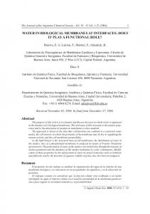
Probing the interfacial water and their interactions with the membranes has always been an experimental challenge, as this layer of water is extremely thin. Although Berkowitz et al have shown, through molecular dynamics (MD) simulations, that this membrane hydration layer extends only up to ∼5 ˚ A from the membrane layer [20]], these simulations depend heavily on the choice of model potentials used in the calculations. It is only imperative that the membrane hydration layer is directly observed through experiments to validate the true nature of these membranes. As a guideline, we can see from the water density profile calculated by MD simulations (shown in figure 1.3), the membrane bound water essentially has several locations along the surface normal as we move towards the bulk. The plot reveals the locations of buried water (region I) near backbone and carbonyl groups of the lipid headgroup, a first external hydration shell (region II) near the phosphocholine group, secondary hydration shells (regions III-IV) and the bulk water (region V).
water density -15 -10 -5 0
II III IV V
5
depth (Å)
I
O O
O O H
O O
P
O
O NH3
10
H
O O
15
Figure 1.3. The water density profile at the DPPC/water interface from MD simulations [20]], is shown on the left. Five distinct regions of interfacial water have been indicated as I-V as a function of the depth (in ˚ A), starting from -15 ˚ A (air), towards 0 ˚ A (phosphate group of the lipid) and finally to 15 ˚ A (bulk water). Region I (-5 to 3 ˚ A) represents location and density of buried water near the carbonyl groups. Region II (3-6 ˚ A) indicates first external hydration shell. Region III-IV (6-12 ˚ A) indicates secondary hydration shells. Region V (>12 ˚ A) indicates bulk water. The cartoon of the hydrated lipid on the right indicates the interfacial water regions, roughly corresponding to the depth scale on the left.
Since directly observing this interfacial water and its role in various complexities of membrane structure/function poses a great experimental challenge, there is no one perfect method for studying 6
such systems. Although it is beyond the scope of this thesis to describe in detail, the wide variety of methods that have successfully been applied to study biological membranes, include time-domain fluorescence (upconversion [40]]or correlation [41]]) spectroscopies, ESR/EPR [42–44]] and NMR (see, e.g. Refs. [45–47]]) studies of membrane dynamics, neutron [37, 48, 49]] and X-ray scattering [50–52]], conventional [53]] and multidimensional infrared [54]] spectroscopies and scanning probe microscopies [55]]. Each of these techniques has its own unique strengths and limitations. In terms of limitations, some of the techniques require a perturbation of the sample due to the local environment necessary for the measurement, such as the elimination of an adjoining liquid water phase (for studies in vacuum), or the stacking of lipid bilayers (e.g. for NMR). Extrapolating such results to biologically relevant conditions clearly requires that the properties of interest do not change as a function of hydration level or headgroup-headgroup interaction. Other techniques may inherently perturb the sample by the means of measurement, for instance by adding a fluorescent label for microscopy, using the tip of a scanning probe microscope, or using high-energy neutrons, X-rays or electrons. Moreover with the existing surface techniques, directly probing such a complex membrane-bound interfacial water non-perturbatively, is almost impossible without compromising on the surface- or molecular-selectivity. In the recent past, the second order non-linear optical techniques of second harmonic generation (SHG) and sum frequency generation [26–30]](SFG) have proven to be a versatile non-invasive labelfree all-optical tool for probing interfaces, especially liquid-liquid interfaces, with excellent molecular and surface specificities. Using vibrational SFG (VSFG), one can probe the vibrational chromophores present in the interfacial molecular moieties, in a background-free, label-free manner. This, as we shall see, is our primary choice of technique to look at the interfacial water.
1.5
Vibrational Sum Frequency Generation (VSFG) Spectroscopy - The Surface Probe
Although a vast number of literature has been written on various nonlinear optical techniques, in this section I introduce some of the basic concepts behind VSFG and its surface and molecular specificity. A comprehensive theoretical treatment of nonlinear optics is beyond the scope of this thesis, but can be followed up in the textbooks of Boyd [56]] and Shen [57]].
1.5.1
Concepts in Nonlinear Polarization
In linear optical phenomena like reflection or refraction, the optical response of the material atoms is linearly proportional to the strength of the externally applied optical field. Nonlinear optical phenomena, on the other hand are nonlinear, in the sense that the optical response of the atoms/molecules in the material depends in a nonlinear manner on the strength of the applied optical field. For instance, second harmonic generation is one of the processes that may occur when the optical response of the material depends quadratically on the applied optical field strength. To quantify the material optical response as a result of the applied optical field, one needs to consider 7
the time-dependent polarization P(r, t) induced in the material, which can be expanded in a Taylor series in terms of the applied field E(r, t) to give, in a simplified notation:
P(r, t) ≡ χ(1) E(r, t) + χ(2) E2 (r, t) + χ(3) E3 (r, t) + ... = P(1) (r, t) + P(2) (r, t) + P(3) (r, t) + ...
(1.1) (1.2)
where χ(1) is the linear susceptibility (or polarizability) - responsible for all linear optical processes; χ(2) and χ(3) are the second-order and third-order optical susceptibilities, respectively - responsible for various nonlinear phenomena like SHG/SFG and third harmonic generation. The induced timedependent polarization P(r, t) in the material acts as a source term for generating new fields and is governed by the optical wave equation that follows directly from Maxwell’s equations in the electric dipole approximation3 −O2 E(r, t) +
4π ∂ 2 1 ∂2 E(r, t) = − P(r, t) c2 ∂t2 c2 ∂t2
(1.3)
The term E(r, t) in this equation 1.3, is the electric field generated in the material as a result of the induced polarization P(r, t). This induced polarization is a sum of the linear and non-linear polarizations in the material as shown in equation 1.4 P(r, t) = P(1) (r, t) + P(NL) (r, t)
(1.4)
where P(1) (r, t) is the linear polarization and P(NL) (r, t) is the non-linear polarization. The nonlinear polarization term is the driving field for various non-linear processes.
1.5.2
Sum Frequency Generation
Sum frequency generation (SFG) is a second-order non-linear optical process in which the secondorder polarization P(2) (r, t) acts as the nonlinear source term P(NL) (r, t) (see eq. 1.4) in Maxwell’s optical wave equation shown in equation 1.3. From equation 1.1, we have seen that the generic second-order polarization term is given by: P(2) = χ(2) E2
(1.5)
When two different optical fields E1 and E2 are applied in a material, the total electric field experienced by the system is: E = E1 + E2
(1.6)
3 Under the electric dipole approximation, the wavelength of the electromagnetic radiation which induces (or is emitted during) transitions between different energy levels, is much larger than the typical size of the material atom, approximated to a dipole. It is assumed that the dipole induced within a molecule is related solely to the applied macroscopic field and that contributions from the dipolar fields of neighbouring induced dipoles may therefore be ignored. In addition, within this approximation, the effects of optical magnetic fields and multipoles are neglected, in order to simplify the Maxwell’s equations in the course of deriving the optical wave equation.
8
where the applied fields have optical frequencies ω1 and ω2 and have the form:
E1
=
E1 cos ω1 t
(1.7)
E2
=
E2 cos ω2 t
(1.8)
Now using the equations 1.6, 1.7 and 1.8 in equation 1.5, P(2) = χ(2) [E1 cos ω1 t + E2 cos ω2 t]2
(1.9)
On expansion of equation 1.9, we get all the possible second order nonlinear optical processes:
P(2) =
χ(2) 2 [E1 + E22 − E12 cos 2ω1 t − E22 cos 2ω2 t + 2E1 E2 cos(ω1 + ω2 )t + 2E1 E2 cos(ω1 − ω2 )t] (1.10) 2
In equation 1.10, the first two terms on the right-hand side, represent frequency-independent optical rectification, the next two represent SHG processes at 2ω1 and 2ω2 optical frequencies, the next one SFG at ω1 + ω2 frequency and the last term difference frequency generation at ω1 − ω2 frequency. Although the simple classical electromagnetic approach adopted here is sufficient to demonstrate the origins of various second-order nonlinear processes, an exhaustive definition is obtainable through rigorous calculations, such as those presented in the textbooks by Shen [57]] or Boyd [56]]. In the following section(s), I shall focus mainly on the SFG component of the second-order polarization, where the generated field has a frequency at the sum of the frequencies of the applied optical fields. We shall also show how to use this nonlinear optical technique as a surface-sensitive optical probe.
1.5.3
Vibrational Sum Frequency Generation at Interfaces
The VSFG experiment is schematically shown in figure 1.4. Experimentally, when two laser beams - one with a tunable mid-IR frequency (λIR ∼3000 nm) resonant with a vibrational mode in the system and the other with a fixed near-IR (visible) frequency (λvis =800 nm) - are overlapped in space and time at an interface and such that the energies and momenta (phase matching) of the incoming and outgoing photons are conserved, vibrational SFG (VSFG) is generated at a visible frequency (λSF ∼630 nm). The energy and momentum conservation (phase-matching condition) of the photons involved in the VSFG process are shown in the relations:
~ωSFG kSFG k
= ~ωIR + ~ωvis
(1.11)
vis = kIR k + kk
(1.12)
where kik is the component of the wavevector of the corresponding photon i parallel to the surface.
9
VIS SFG vO-H = 1 IR vO-H = 0
(a)
(b)
Figure 1.4. (a) Schematic of the Vibrational SFG (VSFG) experiment at an interface. (b) The energy level diagram depicting the VSFG process where the IR frequency is resonant with the 0→1 transition and the visible frequency is non-resonant and simply upconverts the 0→1 transition to generate the SFG signal.
The correct description of the second-order nonlinear polarization in the Cartesian co-ordinates of the lab frame, is given by: (2)
(2)
Pi,SFG = χijk Ej,vis Ek,IR
(1.13)
where i, j and k are indices that correspond to the Cartesian co-ordinates x, y and z (corresponding (2)
to the axes shown in figure 1.4). Pi,SFG denotes the induced polarization in the ith direction due (2)
to the jth and kth components of the applied fields, Ej,vis and Ek,IR , respectively and χijk is the third-ranked second-order macroscopic susceptibility tensor. In the VSFG process, the emitted SFG field, ESFG is phenomenologically related to the induced (2)
second-order polarization Pi,SFG , through the equation: (2)
Ei,SFG = Li Pi,SFG
(1.14) (2)
where Li is the non-linear Fresnel factor associated with Pi,SFG , and it takes into account the geometric (phase matching) considerations of the SFG process - for instance, the polarizations and the angles of the incident applied fields, define the direction of the emitted SFG field.4 4 The electric fields also have Fresnel factors associated with them, usually denoted by K . Essentially equation j 1.13 can be re-written while including the electric field Fresnel factors as: (2)
(2)
Pi,SFG = χijk Kj Ep/s,vis Kk Ep/s,IR
10
(1.15)
The SFG intensity ISFG , which is the square of the emitted SFG field Ei,SFG , is then simply proportional to the square of the induced polarization, as follows:
Ii,SFG ISFG
= |Ei,SFG |2
(1.16)
(2)
= |Li Pi,SFG |2
(1.17)
(2) |Li χijk Ej,IR Ek,vis |2 (2) |Li χijk |2 Ij,IR Ik,vis
= =
(1.18) (1.19)
Therefore, by simply measuring the SFG intensity using certain polarization combinations of the (2)
incoming and outgoing beams, one can estimate the value of χijk for a given material. 1.5.3.1
Properties of χ(2) and surface-sensitivity of VSFG
(2)
χijk is a third-rank tensor, where i, j and k indices represent the Cartesian co-ordinates of the laboratory frame, thus leading to 27 possible susceptibility tensor elements. The macroscopic χ(2) (2)
is related to the molecular second-order hyperpolarizability βλµν (defined in the molecular frame), through: (2)
χijk = N
X
(2) ˆ ˆj · µ h(ˆi · λ)( ˆ)(kˆ · νˆ)iβλµν
(1.20)
λ,µ,ν
ˆ are the unit vectors in the laboratory frame where N is the number density of molecules, (ˆi, ˆj, k) ˆ µ and the (λ, ˆ, νˆ) are the unit vectors in the molecular frame. The angular brackets indicate (2)
averaging over the molecular orientational distribution. Thus, χijk is an orientationally- and number(2)
averaged quantity of the molecular hyperpolarizability, βλµν which is a product of the IR and the Raman transition moments of the molecule. [58]] Both χ(2) and β (2) are third-ranked tensors: third-ranked tensors have the property that they change sign upon an inversion operation in which ˆ Therefore, ˆi → −ˆi, ˆj → −ˆj, kˆ → −k. (2)
(2)
χijk = −χ−i−j−k
(1.21)
For materials or systems possessing inversion symmetry, molecular properties do not change upon inversion operation. Therefore: (2)
(2)
χijk = χ−i−j−k
(1.22)
The only solution that satisfies both the equations 1.21 and 1.22 is: (2)
(2)
χijk = −χijk = 0
(1.23)
For purposes of this section where the electric fields are represented as vectors and not scalar quantities, it is not necessary to discuss the electric field Fresnel factors exhaustively, although a thorough discussion can be found in [58]].
11
This sets the selection rule that SFG is forbidden in any medium/material that possesses inversion (2)
symmetry, where the net χijk = 0 under the electric dipole approximation. The bulk of most liquids or solids is regarded as macroscopically random, i.e. possesses inversion symmetry, and is therefore SFG-inactive. However at surfaces and interfaces the inversion symmetry is broken, thus rendering the near-surface region SFG-active. This makes SFG a very attractive surface-sensitive, backgroundfree probe, particularly for liquid-vapor or liquid-liquid interfaces, as there is no contamination of SFG generated from the bulk. In fact, the surface region probed by SFG can be as small as a few angstroms or less, of course depending on the details of the surface being studied. (2)
Moreover, the non-zero χijk values at the interface contain information about the macroscopic (2)
orientation of surface molecules. There are 27 possible χijk tensor elements which reflect the molecular hyperpolarizability and molecular orientation at the interface. For an interface composed of non-chiral molecules, with an overall azimuthal symmetry, only seven of the 27 elements are non-zero due to symmetry considerations at the interface, of which several are degenerate, finally leading to only four distinct different sets: (2)
(2)
(2)
(2)
(2)
(2)
(2)
χzzz , χxxz (= χyyz ), χxzx (= χyzy ), χzxx (= χzyy ) The magnitudes of the different tensor elements can be determined by using polarization-resolved measurements. Two different polarizations can be investigated for the two incident beams and the SFG beam: one with the electric field vector perpendicular to the plane of incidence, labeled ”s”, and one for the electric field vector parallel to the plane of incidence, labeled ”p”, as shown in figure 1.4. Four polarization combinations of the 3 beams are sufficient to address the four distinct different sets of the seven non-zero tensor elements: PPP, SSP, SPS, PSS, with the letters listing the polarization of the three fields in the order of decreasing frequency, so the first is for the sum frequency, the second is for the visible beam, and the last is for the infrared beam. The four combinations give rise to four different intensities:
(2)
(2)
(2)
IP P P
∝
0 0 0 2 |L0z Lz Lz χ(2) zzz + Lz Li Li χzii + Li Lz Li χizi + Li Li Lz χiiz |
ISSP
∝
|L0i Li Lz χiiz |2
(1.25)
ISP S
∝
(1.26)
IP SS
∝
(2) |L0i Lz Li χizi |2 (2) |L0z Li Li χzii |2
(2)
(1.24)
(1.27) (1.28)
, where index i is of the interfacial xy-plane, and L and L’ are the linear and nonlinear Fresnel factors, respectively which are essentially a function of the beam geometries and angles with respect to the surface normal (which is along the Z-axis in the figure 1.4). 1.5.3.2
VSFG - A surface-specific IR probe
As shown in the previous section, the SFG intensity is essentially a measure of the macroscopic χ(2) :
12
ISFG
∝
|χ(2) |2
(1.29)
In VSFG spectroscopy, the χ(2) can be expressed as a function of the IR frequency ωIR as: χ(2) = ANR eιφNR +
X Aj (N0,j − N1,j ) ωIR − ωj + ιΓj j
(1.30)
Here the nonlinear susceptibility χ(2) , and hence the VSFG signal, is enhanced when the IR frequency is resonant with a vibrational mode j of the surface molecules, as seen in the second term of equation 1.30. By scanning the IR over a range of frequencies, we get the VSFG spectrum of the interface. The amplitude of the resonant SFG signal is given by Aj , which is a function of the population difference between the ground and first excited vibrational states, ∆Nj = N0,j − N1,j . ωIR is the frequency of the incident IR pulse, ωj is the vibrational resonance frequency, and Γj is the linewidth of the j th resonance. Generally, there is also a non-resonant contribution to the overall SFG signal, characterized by amplitude ANR and phase φNR . Although the non-resonant signal can exceed the resonant signal in case of metallic substrates, for the interfaces studied in this thesis, the nonresonant contribution from the sub-phase (either water or D2 O) is generally much smaller than the resonant modes at the interface. Therefore VSFG spectroscopy, with its high sensitivity to molecular-specific vibrational resonances, makes it a surface analogue of IR spectroscopy. Together with its sub-monolayer sensitivity, VSFG technique has proven to be a highly desirable surface tool in the recent past. VSFG is further appealing to the surface science community owing to the relative simplicity in implementation of a basic VSFG setup, that has recently become available commercially [59]]. As a result, the past two decades have seen much work in frequency- and polarization-resolved VSFG devoted to characterizing and understanding various solid-gas, liquid-gas, and liquid-liquid interfaces (see, e.g. [60–78]].)
1.6
Time-Resolved SFG Spectroscopy
By providing the information-rich vibrational spectrum of interfaces in a surface-specific, label-free and background-free manner, frequency-resolved static VSFG studies have created a significant impact in the surface science community. However this static spectroscopy falls short of providing direct information on the dynamics of molecular structures and intra-/intermolecular vibrational coupling, which evolve at ultrafast time scales. IR pump-probe [79,80]] and 2D-IR [81,82]] techniques developed in the recent past, have shown their advantage over static spectroscopy in their ability to directly probe the ultrafast molecular dynamics in bulk systems. Although the first literature on pump-probe SFG experiments using picosecond pulses to probe vibrational lifetimes of adsorbates on semiconductor [83]] and on metal surfaces [84]] appeared in 1990, the time and frequency resolutions and the applicability of the technique to any interface were restricted to picosecond molecular dynamics. With the development of short amplified pulses (∼100 fs) and better detection techniques, broad13
band IR pump - SFG probe experiments with sub-picosecond time resolution have now become a possibility. As a result, sub-picosecond surface vibrational lifetimes and dynamics can be interrogated directly. In the recent past, pump-probe SFG experiments have been performed to study the mechanisms of adsorption and desorption of gases on catalytic metals under UHV conditions [85]]. Recently time-resolved electronic SFG studies have interrogated probe molecules at buried interfaces [86]]. The work presented in this thesis, demonstrates a novel time-resolved SFG (TR-SFG) technique that was developed by combining static broadband SFG spectroscopy with IR pump-probe spectroscopy to study the ultrafast structural dynamics of molecules at the air-water interface and various water-lipid (model bio-membrane) interfaces: an attempt to elucidate the structure and dynamics of water at the model biological interfaces, under normal laboratory conditions. The development of our time-resolved SFG spectrometer was contemporaneous with that in the group of Y. R. Shen, which published the first IR pump - SFG probe results of interfacial water [87]].
VIS vO-H = 1
SFG
τdelay
vO-H = 0 IR pump IR probe
(a)
(b)
Figure 1.5. (a) Schematic of the TR-SFG technique with the indicated pump IR, probe IR, the visible and the SFG beams. (b) The energy level diagram in the presence of a pump pulse which excites molecules to the first vibrationally excited state. The pair of probe pulses generating the SFG beam is scanned in time τdelay with respect to the IR pump pulse. By monitoring the modulation in the SFG signal as a function of time, the evolution of the system can be followed in real-time as molecules relax back to the ground state.
The basic schematic of the pump-probe TR-SFG technique and the energy level diagram is shown in figure 1.5. In a pump-probe TR-SFG experiment, the pump IR pulse excites molecules from the ground state v = 0 to the first vibrationally excited state v = 1 in a two-step process: high intensity IR pump pulse first prepares the two-level system by creating a vibrational coherence between the v = 0 and v = 1 and then population is transferred from v = 0 to v = 1. If the anharmonicity of 14
the vibration is larger than our experimental IR probe frequency window (∼120 cm−1 ), the excited state SFG signal (v = 1 → 2) will not be observed. Moreover, this v = 1 → 2 signal will be very small, given the fact that the SFG intensity depends on the square of the surface population density. This pump-induced population transfer from v = 0 → 1, transiently reduces the effective χ(2) of the system since χ(2) ∼ ∆N , where ∆N is the population difference between v = 0 and v = 1 states. This perturbation in the equilibrium population distribution is observed as a reduction in the SFG probe signal (’bleach’). As the molecules relax back to the vibrational ground state, the equilibrium population distribution is regained: the SFG signal returns to its original magnitude as a function of the delay time between the IR pump pulse and SFG probe pulse pair. In this mode, TR-SFG is fully analogous to the more widely applied transient IR absorption spectroscopy, except for the fact that the latter involves detection of a third-order coherence (two interactions with the pump IR field and one with the probe IR field), while the former involves the up-conversion of the third-order coherence created by the pump and probe IR fields, to a fourth-order coherence by the visible pulse. Hence the TR-SFG technique involves a χ(4) optical interaction while static SFG spectroscopy is a χ(2) process. The time dependence of the fourth-order signal is contained in the population densities of the ground (N0 ) and the excited state (N1 ), such that, in the absence of intermediate states:
ISF G
∝ [N0 (t) − N1 (t)]2
(1.31)
[1 − 2N1 (t)]2
(1.32)
= =
1 − 4N1 (t) +
4N12 (t)
≈ 1 − 4N1 (t)
(1.33) (1.34)
This has some interesting consequences: for example, when the pump excites 10% of the ground state molecules to the excited state at zero pump-probe delay, the population difference amounts to [N0 (t) − N1 (t)]2 = (0.9 − 0.1)2 = 0.64. The SFG intensity level thus decreases to 0.64 and thus a bleach of 36% is observed. We further note that, for sufficiently small N1 , the signal will decay with T1 . This simplified analysis of TR-SFG data is dealt with, in greater detail in Chapter 3.
1.7
Thesis Outline
This thesis is essentially a compilation of various experiments performed using the novel TR-SFG spectroscopy technique. In the next chapter (Chapter 2), I describe the TR-SFG experimental setup in detail. In Chapter 3, I show the results of the first experiments performed using TR-SFG to study the vibrational dynamics of water molecules at the water-air interface. In Chapter 4, I discuss the TR-SFG experiments performed to elucidate the dynamics of water molecules at a variety of lipidwater interfaces. Chapter 5 deals with the TR-SFG studies of water on a model lung surfactant system. In Chapter 6, I describe the studies on the vibrational relaxation dynamics of C-H moieties and the energy flow dynamics across a model membrane system.
15
Chapter
2
Experimental Technique Abstract We present a novel setup to elucidate the dynamics of interfacial molecules specifically, using surfaceselective femtosecond vibrational spectroscopy. The approach relies on a fourth-order nonlinear optical interaction at the interface. In the experiments, interfacial molecules are vibrationally excited by an intense, tunable femtosecond mid-infrared (2500−3800 cm−1 ) pump pulse, resonant with the molecular vibrations. The effect of the excitation and the subsequent relaxation to the equilibrium state are probed using broadband infrared+visible sum frequency generation (SFG) light, which provides the transient vibrational spectrum of interfacial molecules specifically. This IR pump-SFG probe setup has the ability to measure both vibrational population lifetimes as well as the vibrational coupling between different chemical moieties at interfaces. Vibrational lifetimes of interfacial molecules are determined in one-dimensional pump-SFG probe experiments, in which the response is monitored as a function of the delay between the pump and probe pulses. Vibrational coupling between molecular groups is determined in two-dimensional pump-SFG probe experiments, which monitor the response as a function of pump and probe frequencies at a fixed delay time. To allow for one setup to perform these multifaceted experiments, we have implemented several instrumentation techniques described here. The detection of the spectrally resolved differential SFG signal using a combination of a charge-coupled device camera and a galvanic optical scanner, computer-controlled Fabry−P´erot etalons to shape and scan the IR pump pulse and the automated sample dispenser and sample trough height corrector are some of the novelties in this setup.
2.1
Introduction
In this chapter, the experimental setup for time-resolved sum frequency generation (TR-SFG) spectroscopy is presented in detail. The first section describes the scheme for generating high intensity mid-IR pulses (2900-3500 cm−1 ) and the home-built pulse shaper for generating the narrowband visible upconversion pulse (12500 cm−1 ; 800 nm). The second section deals with the instrumentation and device controls at the sample stage. The third section discusses the novel instrumentation utilized in the detection path and acquisition schemes, followed by a fourth section that deals with the electronics, device synchronization and the data acquisition software. Finally, the chapter ends with a section that gets us started with the essentials to perform a TR-SFG experiment.
2.2
Generation of Mid-IR and Visible upconversion pulses for VSFG pump-probe delay
w800
wIR=w800-w2I pump IR generation
1 mJ
OPA/2I generation
w2I
2.5 mJ
w2I
w800
Collimating lens
pump IR 100 µJ
SFG probe IR generation
probe IR 20 µJ
3.5 mJ
Sample
wIR=w800-w2I
pump-on
Oscillator
Spectrograph Regen 800 nm (D12 nm) tp=100 fs
Verdi
Nd:YLF
1 kHz
pump-off PMT boxcar ADC
CCD
galvo mirror
Pulse shaper
Shaped visible upconversion pulse (1µJ, 800 nm)
T
Data acquisition software
Laser system Figure 2.1. TR-SFG Experimental Setup.
The TR-SFG experimental scheme can be seen in figure 2.1. A conventional broadband SFG setup [77]] requires a pair of probe laser pulses, i.e., a weak broadband IR (∼10 µJ, FWHM ∼150 17
cm−1 ) and a narrowband visible upconversion pulse (∼1 µJ, FWHM 50 fs) compared to the traces observed at 3200 cm−1 . Also the initial recovery of the SFG intensity appears to be much slower at these frequencies than at 3200 cm−1 . After this initial relaxation process, a slow relaxation process is also evidently occurring, on timescales of tens of ps. (ii) The zwitterionic lipid/water interface: DPPC and DPPE (a) Response at 3200 and 3300 cm−1 : After the IR excitation, the SFG intensity decreases instantaneously (within ∼50 fs), due to bleaching of the ground state. Subsequently, there is a partial recovery of the SFG signal, after which the signal decreases again, and finally continues to
49
recover to a level that is lower than its original value. The initial dynamics (bleach, partial recovery and second signal decrease) occur on sub-picosecond timescales, whereas the final slow rise occurs over tens of picoseconds. (b) Response at 3400 and 3500 cm−1 : The transients look similar to the ones at the charged lipid/water interface - with an initial delayed bleach after excitation, subsequent relaxation of the bleach within 1 ps, followed by a slow rise in order of tens of ps. No additional signal decrease was observed at these frequencies. The different long-time signal offsets in all the transients at delay times >100 ps can be readily attributed to the spectral shifts due to the IR pump-induced heating: it was verified that the SFG spectrum of the hydrogen-bonded O-H stretch mode shifts to blue frequencies owing to heat-induced weakening of H-bonds.
c2
T12
N1
N2 s0
c3
T23 N3
c0
c4
T34
N4
N0
Figure 4.3. The 5-level kinetic model used in the TR-SFG data analysis. The population of the ith state is denoted by Ni , the absorption cross-section for 0→1 transition is denoted by σ0 , the relative susceptibility of state i is denoted by χi and the i→j time-constant is denoted by Tij .
These transients can be described accurately by a 5-level kinetic model shown in figure 4.3: an extension to the 4-level system used to describe bulk water IR pump-probe transients [131, 136, 142, 143]]. The relevant coupled differential equations describing the population kinetics in such a system can be written as, dN0 (t) dt dN1 (t) dt
=
−I(t, τfwhm )σ0 (N0 (t) − N1 (t))
=
I(t, τfwhm )σ0 (N0 (t) − N1 (t)) −
50
(4.4) N1 (t) T12
(4.5)
dN2 (t) dt dN3 (t) dt dN4 (t) dt
= = =
N1 (t) N2 (t) − T12 T23 N2 (t) N3 (t) − T23 T34 N3 (t) T34
(4.6) (4.7) (4.8)
where, dNx (t) = the rate of population change in level x at time, t dt I(t, τfwhm ) = the Gaussian pump pulse with a certain pulse duration, τfwhm σ0
=
is the absorption cross-section for the 0 → 1 transition
As shown earlier in chapter 3, in our modeling of the TRSFG transient data, the susceptibilities and the relaxation times are kept as fit parameters and the normalized differential SFG signal, ∆ISFG as a function of the pump-probe delay t, is then computed from the time-dependent state populations by,
∆ISFG (t) =
[(N0 (t) − N1 (t))χ0 + χ2 N2 (t) + χ3 N3 (t) + χ4 N4 (t)]2 [N0 (0)]2
(4.9)
This simple model provides an adequate description of the data as will be shown in the following sections for all the lipid/water systems. In contrast to the 4-level model used to describe the IR pump-probe measurements in bulk water [131, 136, 142, 143]], the lipid/water TRSFG measurements require a 5-level model as shown in figure 4.3. The 5-level model can readily be interpreted as follows: infrared excitation of the molecules promotes population from the O-H stretch vibrational ground state v0 , to the first vibrationally excited state v1 . Subsequent vibrational relaxation occurs to a state v2 on a timescale T12 , which can be identified as the vibrational lifetime T1 . State v2 corresponds to the system in which the energy has flowed out of the high-frequency vibrational O-H stretch, but has not yet equilibrated over all degrees of freedom. v2 subsequently relaxes to v3 with a timescale of T23 . v3 corresponds to the situation where the excess energy is equilibrated over all degrees of freedom, following a reorganization of the hydrogen bond network. The timescale associated with the H-bond network rearrangement is T23 . Finally, the increase in temperature results in a change of the hydration state of the lipid monolayer: v3 converts into the slightly different v4 with a timescale of T34 , which is much larger (≥20 ps) than T12 and T23 . Its precise value depends on the monolayer composition. In the following, the different monolayer systems will be discussed one by one. 4.4.2.1
DPTAP/H2 O Interface
The TR-SFG transients for the DPTAP/water interface are shown in figure 4.4. As we can see, the data can be well described with the aforementioned 5-level kinetic model. Previous investigations of the vibrational dynamics of interfacial water at the water-air interface [93]] and the water-silica 51
Figure 4.4. One-colour TR-SFG transients for the DPTAP/water interface recorded at four different IR frequencies indicated in the graph. The left panel depicts the dynamics up to 5 ps; the right up to 20 ps.
interface [87]] have revealed very fast intermolecular energy transfer between water molecules. This very rapid (sub-50 fs) energy transfer leads to a homogeneous response of the different spectral components within the water band. When exciting a weakly hydrogen-bonded water molecule at high frequency (3500 cm−1 ), the excitation can ’hop’ rapidly to a strongly hydrogen-bonded water molecule at low frequency (3200 cm−1 ). Moreover, the excitation is not restricted to the surface; the surface excitation can be transferred to and from the bulk. Therefore, although the intrinsic response may be different for interfacial water molecules with different hydrogen bonds, an averaged response was observed for both the water-air (as shown in chapter 3) and the water-silica [87]] interfaces. It would therefore seem intuitive to attempt to apply a similar model of homogeneous response to water at the water-lipid interface. This implies that the three time constants that describe the transitions between the different states in the 5-level model would be the same for all frequencies. Indeed, three out of four traces for DPTAP - and, as will be shown below, the same is true for the other lipids - can be described using one set of time constants. Remarkably, the 3200 cm−1 data are notably different: the vibrational relaxation time (T12 in the model) is appreciably shorter than that inferred for the other frequencies. The following table 4.1 shows the various time constants extracted from the model: Table 4.1.
DPTAP 3200 cm−1 3300 cm−1 3400 cm−1 3500 cm−1
T12 (fs)