uncorrected proof

Computers and Electronics in Agriculture xxx (2018) xxx-xxx

Contents lists available at ScienceDirect

Computers and Electronics in Agriculture

Original papers

PR OO F

journal homepage: www.elsevier.com

A hybrid finite volume-finite element model for the numerical analysis of furrow irrigation and fertigation Giuseppe Brunettia⁠ ,⁠ ⁎⁠ , Jirka Šimůnekb⁠ , Eduardo Bautistac⁠ a b c

University of California, Davis, Department of Land, Air and, Water Resources, CA 95616, USA University of California, Riverside, Department of Environmental Sciences, CA 92521, USA USDA, ARS, U.S. Arid Land Agricultural Research Center, Maricopa, AZ 85138, USA

ABSTRACT

UN CO RR EC TE D

ARTICLE INFO Keywords: Surface flow Subsurface flow Furrow irrigation HYDRUS WinSRFR

This study presents a hybrid Finite Volume – Finite Element (FV-FE) model that describes the coupled surface-subsurface flow processes occurring during furrow irrigation and fertigation. The numerical approach combines a one-dimensional description of water flow and solute transport in an open channel with a two-dimensional description of water flow and solute transport in a subsurface soil domain, thus reducing the dimensionality of the problem and the computational cost. The modeling framework includes the widely used hydrological model, HYDRUS, which can simulate the movement of water and solutes, as well as root water and nutrient uptake in variably-saturated soils. The robustness of the proposed model was examined and confirmed by mesh and time step sensitivity analyses. The model was theoretically validated by comparison with simulations conducted with the well-established model WinSRFR and experimentally validated by comparison with field-measured data from a furrow fertigation experiment conducted in the US.

1. Introduction

Agriculture is among the most important human activities due to its role in the food supply chain. According to one of the latest FAO reports (FAO, 2017), agricultural production more than tripled between 1960 and 2015. This remarkable expansion has been accompanied with a dramatic increase in the use of irrigation and fertilization, and an associated significant environmental footprint, thus posing important sustainability issues. Irrigation for agricultural purposes accounts for 70% of all water withdrawn from aquifers, lakes, and streams (FAO, 2011a). Furthermore, the worldwide demand for fertilizers has grown by 25% in the last decade, and this trend is expected to continue in coming years (FAO, 2015), increasing the risk of nutrient pollution of water bodies. Thus, the transition towards more efficient and sustainable irrigation and fertigation strategies is necessary. Although slowly replaced by pressurized irrigation in developed regions such as The United States, Europe, and Israel, surface irrigation systems continue to be a preferred irrigation method in developing countries. In 2011, surface systems accounted for 96.8% of irrigated surfaces in Southern and Eastern Asia (FAO, 2011b). In particular, basin and furrow irrigation were the most widespread techniques among farmers. When correctly performed, furrow fertigation can increase the efficiency of fertilizer use and crop fertilizer uptake, compared to traditional techniques (Fahong et al., 2004; Horst et al., 2005;

⁎

Corresponding author. Email address: [email protected] (G. Brunetti)

https://doi.org/10.1016/j.compag.2018.05.013 Received 21 February 2018; Received in revised form 5 May 2018; Accepted 8 May 2018 Available online xxx 0168-1699/ © 2018.

Siyal et al., 2012; Šimůnek et al., 2016a). To be successful, furrow irrigation and fertigation systems should be designed and managed so that the application and distribution of water and fertilizer are efficient and uniform, with minimal surface runoff at the lower end of the field and with minimal deep drainage and leaching below the crop root zone (Šimůnek et al., 2016a). To optimize the performance of furrow irrigation systems, numerical models may play an important role since they represent powerful tools for assessing irrigation and fertigation efficiency. Furrow irrigation and fertigation are coupled surface-subsurface processes. Water and solute are injected at the soil surface at one side of an open channel, hence generating a sharp front that moves along a furrow while water and nutrients infiltrate in the underlying soil. Therefore, furrow irrigation and fertigation are (physically, mathematically, and numerically) described as coupled three-dimensional flow and transport processes in both surface and subsurface domains. Nevertheless, solving a fully coupled system of 2D Shallow Water and 3D Richards equations would require significant computing resources and would also likely pose substantial stability issues, mainly stemming from the high nonlinearity of the governing equations. This presents a problem in the modeling of flooding and drying processes over porous beds. Therefore, several models have been proposed in the literature that reduce the numerical complexity of a fully 3D model. Katopodes and Strelkoff (1977) used a dimensionless formulation of the governing equations to show that

G. Brunetti et al.

PR OO F

(surface flow and transport occur only during irrigation events), subsurface processes are continuous (subsurface flow and transport continues between irrigation events). Therefore, a fix grid for the subsurface domain is usually used, and values of interest (e.g., infiltration, soil moisture, pressure head, etc.) need to be interpolated between surface nodes, thus leading to a hybrid Lagrangian-Eulerian approach. Nevertheless, results have proven to be fairly sensitive to the interpolation strategy (Wöhling et al., 2006). Lazarovitch et al. (2009) applied the moment analysis techniques to describe the spatial and temporal subsurface wetting patterns resulting from furrow infiltration and redistribution. Furthermore, most of the existing models are based on the finite difference method (e.g., Tabuada et al., 1995; Abbasi et al., 2003; Perea et al., 2010), which can yield spurious oscillations at flow discontinuities unless first-order accurate (upwind) schemes or artificial dissipation are employed. Godunov-type Finite Volume (FV) schemes have been successfully applied to simulate overland flow over pervious and impervious lands (Bradford and Katopodes, 2001; Bradford and Sanders, 2002; Brufau et al., 2002; Burguete et al., 2009; Dong et al., 2013). The FV schemes solve the integral form of the overland flow and solute transport equations, thus being mass conservative both globally and locally. Numerical fluxes are evaluated at the cell faces, thus guaranteeing a straightforward and efficient treatment of the dry bed problem by allowing for flooding and drying of fixed computational cells. Furthermore, numerical oscillations near discontinuities can be eliminated using flux limiters (Bradford and Katopodes, 2001). However, their application to furrow irrigation and fertigation has been rather limited and has not involved a coupled mechanistic description of the subsurface domain. Thus, the main goal of this study is to develop and validate a hybrid Finite Volume-Finite Element (FV-FE) reduced-order model capable of describing coupled surface-subsurface flow and transport processes involved in furrow fertigation. The proposed numerical approach combines a one-dimensional FV description of coupled water flow and solute transport in the surface domain with a two-dimensional mechanistic FE description of flow and transport in the variably-saturated zone, thus reducing the dimensionality (3D) of the problem and associated computational cost. The modeling framework includes the widely-used FE model, HYDRUS-2D, whose numerical features significantly increased the overall modeling flexibility. The proposed model is the first attempt to include HYDRUS-2D in a coupled surface-subsurface furrow fertigation model, thus representing a new contribution to this field. The problem is addressed in the following way. First, the hybrid FE-FV model is theoretically validated against the well-established model WinSRFR (Bautista et al., 2009) using synthetic validation scenarios. Preliminary mesh and time step sensitivity analyses are performed to evaluate the accuracy and the robustness of the proposed numerical approach. Next, the model is validated against measured data from an experimental facility in California, US.

UN CO RR EC TE D

when the Froude number is small, which is typical under irrigation conditions, the inertial terms in the shallow water equations are negligible. With this in mind, they developed the first zero-inertia model for irrigation (Strelkoff and Katopodes, 1977). In the early 80s, Walker and Humpherys (1983) proposed a furrow irrigation model based on a 1D kinematic wave (KW) approximation of open channel flow coupled with the modified Kostiakov equation describing the infiltration process. While the model was assessed against experimental data with satisfactory results, the adoption of the KW equation limited its application to open-ended furrows. Furthermore, the model did not include any description of the subsurface water dynamics. Later on, Oweis and Walker (1990) replaced the KW approximation with the one-dimensional (1D) zero-inertia (ZI) equation, which represents a more realistic approximation of the Shallow Water equations. A more detailed fertigation model was first proposed by Abbasi et al. (2003) and later improved by Perea et al. (2010). In these two studies, water flow and solute transport in an open channel were described using the 1D Zero-Inertia and advection-dispersion equations, respectively. The modified Kostiakov equation was used to calculate infiltration at each time step. Although the model was verified with good results against experimental data from four experimental sites, subsurface flow processes were again neglected. To provide a better and more complete description of coupled water flow and solute transport in the soil, several other models have been proposed in the literature. For example, Zerihun et al. (2005) coupled the 1D zero-inertia equation with the HYDRUS-1D model (Šimůnek et al., 2016b), which numerically describes water flow and solute transport as well as root water and nutrient uptake in 1D variably-saturated porous media. The computational framework, which targeted basin irrigation, was based on the iterative coupling between the surface and subsurface models and was validated against measured data with good results. Ebrahimian et al. (2013) extended this concept to furrows by coupling a 1D furrow fertigation model with the two-dimensional HYDRUS-2D model (Šimůnek et al., 2016b). The coupled model satisfactorily reproduced the overland transport as well as the solute transport in the soil profile. However, the surface and subsurface components were solved separately, leading to an uncoupled numerical framework. As pointed out by Furman (2008), theoretically, the higher the level of coupling, the higher the solution accuracy. This is mainly due to the high nonlinearity of the involved processes, as well as to their different time scales. For instance, overland flow is generally faster than infiltration, thus requiring a different temporal resolution. This temporal misalignment poses significant numerical issues since an approximation is needed to couple surface and subsurface flow. The accuracy of this approximation strongly influences the conservativeness of the numerical scheme. Similarly, the overland solute transport needs to be solved simultaneously with water flow in order to preserve the monotonicity of the solution. One of the most complete furrow irrigation models was developed by Wöhling et al. (2004). The proposed computational framework iteratively coupled a 1D analytical zero-inertia equation with HYDRUS-2D, thus providing a complete description of surface-subsurface water flow along the furrow. The model was further developed and extended by Wöhling et al. (2006), Wöhling and Mailhol (2007), and Wöhling and Schmitz (2007). A similar approach was used by Tabuada et al. (1995), who coupled a model based on a complete hydrodynamic equation of overland flow with a two-dimensional Richards equation. While accurately simulating water flow, neither of the models discussed above considered solute transport in surface and subsurface domains, thus restricting their applicability to irrigation. Hence, further development of similar approaches that would include a detailed description of solute transport in the root zone is desirable for both scientists and practitioners (Ebrahimian et al., 2014). Most of the existing furrow irrigation models adopt a Lagrangian approach, which uses a computational grid that moves along with the wet/dry interface. Although elegant and accurate, this type of approach can lead to coupling issues between the surface and subsurface models, mainly because the grid must be regenerated each time the wet/dry interface moves, and the computational nodes often must be added during flooding or removed during recession to reduce grid distortion error. However, while surface processes are discontinuous


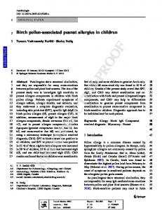
2. Materials and methods 2.1. Modeling approach The proposed approach combines a one-dimensional description of coupled water flow and solute transport in an open channel with a two-dimensional description of variably-saturated water flow and solute transport in soil. As in previous studies (e.g., Tabuada et al., 1995; Wöhling et al., 2004), a key assumption in the model is that the transport processes in the soil domain occur only in the vertical plane, as a function of conditions at a surface flow cross section, and independent of conditions upstream or downstream from that cross section. However, the main novelty of the present study is the development of a complete furrow fertigation model, as well as the inclusion of a widely used hydrological model, HYDRUS, in the modeling framework. The furrow of length L is discretized into N elements, each one characterized by a two-dimensional vertical cross-section (Fig. 1). The open channel cross-section is assumed trapezoidal, although the numerical approach can be easily adapted to other geometries as well. The interface between the surface and subsurface domains acts as a common


UN CO RR EC TE D

PR OO F

G. Brunetti et al.

Fig. 1. A schematic of the modeled transport domain consisting of the trapezoidal open channel and soil (Qi⁠ nj is the solute injection rate [L3⁠ /T], Ci⁠ nj is the solute concentration [M/L3⁠ ], Qi⁠ r is the irrigation inflow rate [L3⁠ /T], ET is evapotranspiration, P is precipitation, h is the water depth in the furrow, hm ⁠ ax is the maximum allowed water depth in the furrow, bw ⁠ is the furrow bottom width, Tw⁠ is the top width, Rw⁠ is the ridge width, FS is the furrow spacing, SS is the side slope, L is the length of the furrow, and dx is the discretization length). The two figures at the bottom show boundary conditions for water flow and solute transport.

2.2. One-dimensional overland flow and solute transport

2.2.1. Governing equations The one-dimensional overland system can be described in the conservative form (Burguete et al., 2009) using the cross-sectional water and solute mass conservation, momentum balance, and infiltration as follows:

(1)

(2)

where U is the vector of the conserved variables, F is the flux vector, S is the source term vector, I is the infiltration vector, and D is dispersion. Vectors can be expressed as:

⁠ 1 where A is the wetted area [L2⁠ ], Q is the discharge [L3⁠ T− ], C is ⁠ 3 the cross-sectional average solute concentration [ML− ], g is the grav⁠ 2 ⁠ 1 itational acceleration [LT− ], S0⁠ is the bed slope [LL− ], Sf⁠ is the − ⁠ 1 3 ⁠ − ⁠ 1 friction slope [LL ], i is the infiltration rate [L T ], Kx⁠ is the dis⁠ 1 persion coefficient [L2⁠ T− ], and I1⁠ and I2⁠ are pres

3

G. Brunetti et al.


sure forces. It must be emphasized that the infiltration rate i is estimated using the HYDRUS-2D model. Since flow velocities in furrow irrigation are typically small, the resulting Froude number is generally less than 0.3. Under such conditions, the inertial terms are negligible and the shallow water equations can be simplified to the well-established zero-inertia (ZI) approximation (Strelkoff and Katopodes, 1977):

2008). The integral form of Eq. (6) was written as: (7)

PR OO F

Application of the divergence theorem to the second term in Eq. (7) produces:

(3) where h is the water depth [L], m is the Manning roughness coefficient ⁠ 1/3], W is the wetted perimeter [L], and c is a units coefficient [TL− u ⁠ (=1.0 in SI units). The 1D unidirectional discharge Q can be obtained from Eq. (3), and is expressed as:

(8)

The contour integral in Eq. (8) was approximated using numerical fluxes F at the edge of each cell j, thus leading to: (9)

One of the main drawbacks of the FVM is the introduction of artificial diffusion in the solution when first-order numerical schemes are adopted (e.g., upwind). Indeed, while preserving the monotonicity of the solution (Godunov, 1954), first-order numerical schemes have lower accuracy compared to the higher-order schemes (e.g., central difference). However, the latter are prone to numerical oscillation (e.g., van Genuchten, 1976, 1978). Therefore, to increase the numerical accuracy while preserving the stability of the numerical solution, a high-resolution scheme was adopted in this study. In this study, the Monotone Upstream-Centered Scheme for Conservation Laws (MUSCL) (van Leer, 1979) was used to spatially discretize the coupled water-solute equations in the conservation form (Eq. (1). The MUSCL methods switch from the first-order scheme in regions with sharp fronts to the higher-order schemes in areas with a relatively smooth solution, thus simultaneously increasing the overall accuracy and avoiding non-physical oscillations. A flux limiter was used to constrain the value of the spatial derivative around sharp discontinuities. In the present study, the van Leer (1974) flux limiter was used in conjunction with the upwind and central differencing schemes. The upwind and central fluxes for overland water flow were expressed as:

UN CO RR EC TE D

(4)

⁠ 1], and k is the channel conwhere J is the hydraulic head loss [LL− ⁠ 1]. veyance [L3⁠ T− The solute advection-dispersion equation

(5)

was simplified as well by considering only the advective component (Eq. (5), as suggested by Strelkoff et al. (2006). In that study, the results of the pure advection equation were compared with the results of the full ADE for different modeling scenarios. The results indicated that the former formulation was able to provide a sufficiently accurate description of the solute distribution along the furrow, although the effects of the longitudinal dispersion were appreciable, especially for blocked-end furrows. Neglecting the dispersion component simplifies the computational scheme and the implementation of boundary conditions. Considering the above-described simplifications, Eq. (2) was rewritten as:

(10)

(6)

where the 1D cell centered discharge Q was expressed as:

2.2.2. Spatial discretization Overland water and solute transport were solved numerically using the Method of Lines (MOL). The MOL approach replaces the spatial derivatives in the Partial Differential Equations (PDEs) with an algebraic approximation, which reduces the PDE to an Ordinary Differential Equation (ODE). Central to the MOL is the numerical approximation of spatial derivatives. In the present study, the Finite Volume Method (FVM) was used to spatially discretize the surface domain. The FVM is a well-established and widely used numerical solution method for a variety of engineering problems involving PDEs, mainly because of its conservativeness. It has been applied successfully in many studies focused on overland flow and solute transport (e.g., Lal, 1998; He et al.,

(11)

It is worth noting that channel conveyance and bed slope were both represented with the arithmetic mean of nodal values. Preliminary simulations confirmed that this type of approximation combined with the MUSCL scheme leads to more accurate results compared to a fully upwind discretization of k and S0⁠ , which introduces significant numerical diffusion in the solution. The same discretization is used for the solute transport. Hence, the numerical flux F obtained using the MUSCL scheme can be written as:

4

G. Brunetti et al.


where Δti⁠ nt is the internal time step calculated by the adaptive RKDP algorithm. To increase the overall computational efficiency of the modeling framework, a specific numerical treatment of the infiltration component is adopted here. As discussed above, the RKDP algorithm uses a fine temporal discretization near discontinuities, implying that the calculation of infiltration (i.e., HYDRUS executions) is carried out with very small time steps, which consequently increases the computational cost. However, the infiltration vector I of Eq. (3) mathematically represents a source/sink term, which is characterized by a moderately low stiffness. Thus, a first-order explicit approximation of infiltration (Brufau et al., 2002) is used in our model, which reduces the number of HYDRUS-2D executions while maintaining a good accuracy. This leads to a mixed explicit time scheme, which uses a 4th order-accurate RKDP time-stepping strategy for the coupled water-solute transport and a first-order explicit scheme for the infiltration term. Practically, this is accomplished by dividing the simulation duration into equal time steps Δt. At the beginning of each time step, the values of the water depth are passed to HYDRUS-2D, which calculates the amount of infiltrated water during Δt. Next, the vector I is inserted in Eq. (1), which is solved by the RKDP method by adapting an internal time step Δti⁠ nt depending on the solution. At time t = 0, the surface domain is solved assuming zero infiltration. Eq. (15) can now be rewritten by including the infiltration term:

(12)

PR OO F

⁠ 1], which was expressed as: where ϕ is the van Leer flux limiter [LL−

(13)

where r is a function that monitors the gradients of the solution and that can be written as: (14)

UN CO RR EC TE D

where u is a dependent variable, which in our case can be the wetted area A for water flow or a cross-sectional average solute concentration C for solute transport. Based on Eq. (12), the first-order monotonicity preserving upwind was adopted in regions characterized by steep gradients in the solution, while the higher-order central differencing scheme was used in regions with a relatively smooth solution, thus increasing the stability and accuracy of the spatial scheme. To facilitate the handling of the downstream boundary condition, the upwind scheme was used to compute the numerical flux in the last cell (i.e., j = N). An upwind discretization was also used for the infiltration term.

(16)

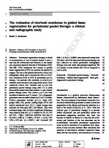
The temporal discretization is depicted in Fig. 2. The non-iterative coupling with the external HYDRUS-2D model significantly decreases the computational cost. However, it must be noted that an ad hoc sensitivity analysis is recommended for the choice of Δt. Since Eq. (16) is solved explicitly in time, the Courant-Friedrichs-Lewy (CFL) stability condition must be respected. In particular, the maximum allowable Δti⁠ nt calculated by the RKDP algorithm must be:

2.2.3. Temporal discretization Once the spatial discretization is defined, time t remains the only independent variable. Since the infiltration component in Eq. (5) is calculated externally using HYDRUS-2D at each time step, and HYDRUS-2D has its own time-stepping algorithm, the computational efficiency of the numerical scheme is strictly related to the frequency of data exchanges between the surface and subsurface models, which dramatically increases when fully implicit time stepping schemes are adopted. Nevertheless, it must be further emphasized that fully implicit schemes, while generally increasing the stability of the computational framework, are only first-order accurate in time. Thus, due to aforementioned considerations about accuracy and computational efficiency, the fourth-order explicit Runge-Kutta Dormand-Prince (RKDP) (Dormand and Prince, 1980) is adopted here to solve the coupled water-solute transport in the trapezoidal channel. More specifically, an RKDP algorithm with an adaptive time-stepping strategy based on the truncation error control is used. This kind of temporal discretization automatically adjusts the time step depending on the solution, thus providing a dense temporal output near discontinuities. It is worth noting that the ZI equation for water flow can be solved separately from the solute advection equation. However, the solute advection equation depends on the wetted area and flow velocity, leading to a one-way coupled system of ODEs. More specifically, the temporal variability of the wetted area strongly influences the solute advection. Thus, a high temporal resolution scheme for water flow is needed to avoid overshooting as well as inaccuracies in the solution of solute advection. The basic method will be first described for the pure conservation law, that is, without source terms. These terms will be incorporated next and required modifications will be indicated as needed. Eq. (10) can now be written as:

(17)

where Γ is the top width of the water flow [L]. Furthermore, the conservativeness of the scheme is checked by monitoring the Relative Mass Balance Error (RMBE) for both water and solute at the end of each time step, which is calculated as:

Fig. 2. A schematic of the temporal discretization.

(15)

5

G. Brunetti et al.


PR OO F

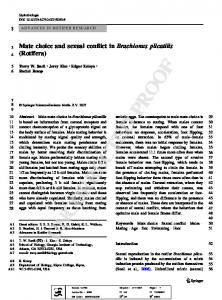
This nonlinear equation was solved for hg⁠ host using the Brent algorithm (Brent, 1974) at each time step. The open end boundary condition was implemented by allowing water to flow over a brink at the end of the furrow. The procedure, which is followed in this study, is similar to the one reported in Soroush et al. (2013). Soroush et al. (2013)(18) showed that, independently from flow conditions, the upstream flow passed over the brink with a depth hb⁠ lower than the critical depth hc⁠ . This phenomenon was previously investigated by Beirami et al. (2006), who indicated that for trapezoidal channels hb⁠ ≈ 0.75hc⁠ . Hence, in the present study, hg⁠ host is determined at each time step by interpolation so that hb⁠ = 0.75hc⁠ (Fig. 3). Both the blocked and open end BCs are applied only when the value of h in the last cell is greater than 0.001 m. To avoid convergence issues, if h < 0.001 m, the water depth in the ghost cell, hg⁠ host, is set equal to hj⁠ =N. The solute advection equation requires the implementation of the boundary condition only on the inflow side of the domain. In the conservation form, this was accomplished by matching the numerical flux with the solute injection rate Qi⁠ nj∙Ci⁠ nj (Fig. 1).

i⁠ are, respectively, the water volume and solute mass where Vi⁠ W ⁠ and V S ⁠ 0 ⁠ per unit length in the soil profile at time i, with V0⁠ W ⁠ and V S ⁠ the corresponding quantities at the beginning of the simulation. The last two terms at the numerators of Eq. (18) indicate the water, qs⁠ oil, and solute, qs⁠ oil c, fluxes across the bottom of the soil domain (e.g., deep percolation and solute leaching).

2.2.4. Boundary conditions The problem statement is completed by the definition of the boundary conditions (BCs) at the two sides of the numerical domain. In the present study, the ghost cells methodology is used (LeVeque, 2002). The 1D ZI equation requires the definition of two BCs, namely inflow and outflow. The specified inflow Q(0,t) determines the numerical flux entering the domain on the left face of the first discretized volume. Two types of BCs can be used for the outlet depending on the type of the furrow end. Since the adopted spatial stencil spans two adjacent cells, the value of the wetted area A in the right ghost cell has to be adjusted at each time step to match the desired BC. If the furrow downstream end is blocked, no outflow is allowed until the water level reaches the maximum furrow depth. If h > hm ⁠ ax (Fig. 1), the model automatically switches to a free overfall BC. Thus, the ghost cell value has to be set so that the numerical flux in the last cell (i.e., j = N) is zero. Considering that the upwind scheme is used for the rightmost numerical flux, Eq. (12) mathematically reduces to Eq. (19):

2.3. Two-dimensional subsurface flow and solute transport

UN CO RR EC TE D

2.3.1. Governing equations The HYDRUS (2D/3D) (Šimůnek et al., 2016b) software simulates water flow and solute transport in variably-saturated porous media. The software describes water flow using the Richards equation for multi-dimensional unsaturated flow (Eq. (7): (20)

⁠ 3], t is time [T], z is the where θ is the volumetric water content [L3⁠ L− vertical coordinate [L], yi⁠ are the spatial coordinate [L], ψ is the soil ⁠ 1], and K are pressure head [L], K is the hydraulic conductivity [LT− i⁠ j components of the hydraulic conductivity anisotropy tensor. Since we assumed isotropic porous media with y1⁠ = y and y2⁠ = z being the transverse (horizontal) and vertical coordinates, respectively, the conductivity tensor is diagonal with the Ky⁠ y and Kz⁠ z entries equal to one. Solute transport is described using the advection dispersion equation:

(19)

(21)

⁠ 3], q is the water velocity where c is the solute concentration [ML− i⁠ − ⁠ 1 [LT ], and

Fig. 3. A schematic showing the linear interpolation of the water depth in the ghost cell when the free overfall BC is used. 6

G. Brunetti et al.


2.3.2. Soil hydraulic properties The van Genuchten–Mualem (VGM) model (van Genuchten, 1980) was used to describe the soil hydraulic properties in this study:

2.4. Models coupling strategy 2.4.1. Wet/Dry boundary tracking In all numerical simulations, the water front is not considered as a moving boundary, and calculations are carried out in both wet and dry cells. The numerical treatment of wet/dry cells is similar to Bradford and Sanders (2002), Bradford and Katopodes (2001) and Brufau et al. (2002). In order to avoid numerical problems associated with extremely low values of the water depth at the advancing front, a threshold value ε is used to identify wet cells. In the present study, water levels above 0.0001 m indicate wet cells (Bradford and Katopodes, 2001). If hj⁠ > ε, the water depth value is passed to HYDRUS, which calculates infiltration that is then used to solve surface flow. Two computational procedures can be followed when the cell is dry: 1. Subsurface in steady-state conditions: HYDRUS is completely bypassed and infiltration is set to 0. For example, during the advance, the last part of the furrow is not simulated, since it is flagged as “dry” and the subsurface flow is negligible. It is worth noting that this option, while increasing the computational efficiency of the numerical scheme, can be considered only when the initial condition is in hydrostatic equilibrium and boundary fluxes are negligible. 2. Subsurface in dynamic conditions: These computations apply during recession. Although no more water infiltrates, HYDRUS can continue to simulate variably-saturated water flow and solute transport in the soil. In such circumstances, a negative pressure head is assigned to the top BC in HYDRUS, which automatically switches to “Atmospheric BC.” HYDRUS is then executed, and the final soil condition is stored and used in the next step.

UN CO RR EC TE D

(22)

was set on top and bottom of the numerical domain to simulate the concentration flux along the boundaries (red lines in Fig. 1).

PR OO F

⁠ 1). Eq. (10) is valid for Di⁠ j are components of the dispersion tensor (L2⁠ T− non-reactive transport, thus adsorption and precipitation/dissolution of the solutes are currently ignored. Note that although HYDRUS-2D considers multiple chemical reactions (e.g., sorption and degradation), this study is limited to non-reactive solutes. HYDRUS advances the solution in time using a fully implicit, temporal discretization scheme for the Richards equation and the Crank-Nicholson scheme for the advection-dispersion equation. The program also uses an adaptive time-stepping strategy to increase the overall computational efficiency.

(23)

⁠ 3], α is a shape parameter rewhere Θ is the effective saturation [L3⁠ L− ⁠ 1], θ and θ are lated to the inverse of the air-entry pressure head [L− s⁠ r⁠ ⁠ 3], n is a the saturated and residual water contents, respectively [L3⁠ L− pore-size distribution index [–], Ks⁠ is the saturated hydraulic conductiv⁠ 1], and l is the tortuosity and pore-connectivity parameter [–]. ity [LT−

2.3.3. Numerical domain and boundary conditions The soil computational domain was discretized using triangular 2D finite elements. In the example simulations discussed below, no mesh stretching was used, and the finite element (FE) mesh was assumed isotropic. The quality of the FE mesh was assessed at each time step by monitoring mass balance errors, which were always below 1% during numerical simulations, indicating a good spatial discretization. The boundary conditions used to simulate solute and water infiltration are reported in Fig. 1. The ‘Atmospheric’ boundary condition, which is assigned to the furrow ridge (green1⁠ lines in Fig. 1), can exist in three different states: (a) precipitation and/or potential evaporation fluxes, (b) a zero pressure head (full saturation) during ponding when both infiltration and surface runoff occur, and (c) an equilibrium between the soil surface pressure head and the atmospheric water vapor pressure head when atmospheric evaporative demand cannot be met by water fluxes towards the soil surface. Due to symmetry, the nodes representing the left and right boundary of the subsurface domain are set as ‘no flux’ boundaries (grey lines in Fig. 1) because no flow or solute transport occurred across these boundaries. A hybrid Dirichlet/Neumann (variable pressure/zero flux) BC was assigned to the border of the trapezoidal channel (orange lines in Fig. 1) to simulate variations of the water depth in the furrow. The specified value of the pressure head (i.e., the water level) was assigned to the channel bed and the pressure heads in other channel nodes are determined by the software based on their elevation relative to the channel bed. A Dirichlet BC was used at nodes with positive pressure heads and an atmospheric BC was assigned to nodes with negative pressure heads (i.e., above the water table). A ‘Third Type’ Cauchy BC

1 For interpretation of color in Fig. 1, the reader is referred to the web version of this article.

2.4.2. Model implementation The one-dimensional horizontal domain representing the furrow and the two-dimensional cross-sectional domains representing the subsurface (Fig. 1) were coupled using a Python script. The script simultaneously solves overland flow and solute transport in the furrow, interacts with HYDRUS-2D, and exchanges data between two models. A series of user-defined functions were developed to write and read the input/output files generated by HYDRUS-2D, which was directly executed from Python, bypassing the HYDRUS (2D/3D) graphical user interface. The coupling strategy is summarized below: 1. The geometric characteristics of the furrow, soil hydraulic properties, initial conditions and other input data are defined in both Python and HYDRUS-2D. The HYDRUS model is then initialized. 2. The horizontal domain is discretized into N homogenous Finite Volumes. There is a HYDRUS-2D cross section for each FV. Pressure head, water content, and solute concentration distributions in the soil are stored in three matrices, which are overwritten at each time step. Water content is stored only for visualization purposes and not used directly in the coupling procedure. Similarly, vectors containing wetted areas, water depths, and solute concentrations in the surface domain are updated at each time step in three additional matrices, in addition to two columns to handle ghost cells. 3. As described above, the MOL is used to reduce the PDEs to a set of ODEs using the FVM. Boundary conditions are applied using ghost cells and the time step dt is set. 4. A for loop is used to iterate through time. At each time step, vectors h and C containing previously calculated values of water levels and solute concentrations in the furrow, respectively, are passed to HYDRUS-2D to setup its boundary conditions. Soil pressure head and solute concentration distributions calculated at the previous time step are used as initial conditions in HYDRUS for the current time step. 5. Another for loop is used to iterate through space and calculate the infiltration vector. Calculated soil pressure heads and solute concentrations are

G. Brunetti et al.


2.5. Theoretical validation

2.5.3. Description of validation scenarios Preliminary sensitivity analyses help identify the most efficient spatial and temporal discretization. The next step is to properly validate the model theoretically and experimentally, which involves the assessment of the model structure and its capacity to accurately describe the investigated system (Sargent, 1998). The former is usually accomplished by comparing the results of the proposed model with the results of a well-established, previously validated model using different synthetic scenarios, thus avoiding the interference of different sources of uncertainty typical of experimental data. In this study, the proposed hybrid FE-FV coupled water and solute transport model was theoretically validated against the solute transport component of the WinSRFR software package (Bautista et al., 2009). This software will be released to the general public with WinSRFR, Version 5.1. The open-channel flow simulator in WinSRFR (Bautista et al., 2009), SRFR, utilizes a 1D zero-inertia approximation of the hydrodynamic wave model, which is coupled with the solution of the 1D advection-dispersion equation for solute transport (Perea et al., 2010). In the present study, the dispersion component was neglected and only advection was simulated using WinSRFR. The explicit infiltration function of Warrick et al. (2007), modified by Bautista et al. (2014) and Bautista et al. (2016) was used to calculate the flow-depth dependent furrow infiltration. This function has been shown to approximate the solution to the two-dimensional Richards equation reasonably well. The pressure head at the wetting front ψf⁠ [L] is calculated using the unsaturated hydraulic conductivity function and can be expressed as:

UN CO RR EC TE D

2.5.1. Mesh sensitivity analysis Schlesinger et al. (1979) defined model validation as a “substantiation that a computerized model within its domain of applicability possesses a satisfactory range of accuracy consistent with the intended application of the model.” There exists a variety of validation techniques that can be used to assess the model accuracy and robustness (Sargent, 1998). Even so, a sensitivity analysis on internal model parameters (e.g., mesh size, time step) represents the first step in a validation framework, sometimes referred to as model verification, that is usually accomplished before using the model itself. The computational mesh size is an important component of Eulerian modeling frameworks, especially when the FVM is adopted, since it is directly related to false numerical diffusion and accuracy. In regions of the computational domain where the dependent variables exhibit sharp gradients, a fine mesh is needed to avoid smearing the solution. However, as the mesh resolution increases, so does the computational cost. The mesh resolution should, thus, be properly designed to simultaneously minimize the execution time and maximize the numerical accuracy. To this end, a mesh sensitivity analysis represents an important prognostic tool. The influence of the spatial discretization N on both the computational cost and the accuracy of the proposed hybrid FE-FV furrow fertigation model is investigated first. The effect of three different mesh sizes (i.e., dx = 2, 5, 10 m) on the simulated water and solute flow in a 100 m long blocked-end furrow (a blocked end scenario in Table 1) is examined. For each numerical simulation, the execution time provides the measure of the computational effort. A time step dt = 20 s was assumed.

Euler approximation of the infiltration component is supposed to deteriorate when the time step dt increases. The loss of accuracy is directly related to the stiffness of the infiltration term, which depends on the scenario analyzed. Therefore, the influence of the temporal discretization dt was investigated using three different time steps (dt = 10, 20, 30 s). The blocked-end furrow described in Table 1 was used as a test case. For each numerical simulation, typical hydraulic information was calculated (i.e., front advance, profiles, etc.) and the execution time was analyzed. A mesh size dx = 5 m was assumed. It must be emphasized that, in the developed computational framework, the time step dt influences not only the computation of infiltration, but also the exchange of information between the surface and subsurface models. On the other hand, the time step does not influence the numerical solution of the zero-inertia and advection equations, which are solved using the RKDP with an adaptive time stepping strategy.

PR OO F

stored for the next time step. The coupled ODEs are solved simultaneously using the RKDP algorithm, and new wetted area, water level, and solute concentration vectors are updated in their respective matrices.

2.5.2. Time step sensitivity analysis A core assumption of the proposed modeling framework is the explicit linearization of the infiltration vector in Eq. (7). As mentioned above, this assumption eliminates the need for an iterative execution of HYDRUS-2D, thus reducing the overall computational cost. However, the accuracy of the forward

Table 1 Geometric characteristics, soil hydraulic properties, and other input parameters used in theoretical validation. Blocked end

Furrow length, L (m) Bottom width, bw⁠ (cm) Side slope, SS (–) Maximum depth, hm ⁠ ax (cm) Bed slope, S0⁠ (–) Manning’s coefficient, m (s/m1⁠ /3) Residual water content, θr⁠ (m3⁠ /m3⁠ ) Saturated water content, θs⁠ (m3⁠ /m3⁠ ) Retention function shape parameter, α (1/cm) Retention function shape parameter, n (–) Saturated hydraulic conductivity, Ks⁠ (cm/min) Tortuosity, l (–) Initial water content, θ0⁠ (m3⁠ /m3⁠ ) Wetting front pressure head, ψf⁠ (cm) (Warrick et al., 2007) Inflow rate, Qi⁠ r (l/s) Solute injection rate, Qi⁠ nj (l/s) Inflow concentration, Ci⁠ nj (g/l) Longitudinal dispersivity (cm), DL⁠ Transverse dispersivity (cm), DT⁠ Irrigation cutoff time, tw⁠ (min) Solute cutoff time, ts⁠ (min)

100 16 1.2 15 0.0005 0.04 0.065 0.41 0.075 1.89 0.074 0.5 0.085 −5.4 2 0.014 40 0.5 0.1 30 30

Open end

0.001

(24)

Two synthetic scenarios were developed to validate the hybrid FV-FE model under different conditions. The first scenario consists of a blocked-end furrow, with a small slope and equal water and solute cutoff times. The second scenario considers an open-end furrow, characterized by a moderate slope and different water and solute cutoff times. In both cases, the soil is assumed to be a sandy loam. The VGM parameters used in HYDRUS-2D are taken from Carsel and Parrish (1988). The subsurface vertical domain is discretized into 2043 triangular elements and 1076 nodes. The effect of groundwater is not simulated in this study and thus a ‘Free Drainage’ BC is assigned to the bottom nodes (z = −80 cm) (blue line in Fig. 1). The geometric characteristics, soil hydraulic properties, and other input parameters are reported in Table 1. 2.6. Experimental validation

20

Theoretical validation provides a first assessment of the model accuracy and robustness. However, the main objective of a numerical model is to accurately reproduce the behavior of the system under investigation. In this view, experimental validation, which compares model results and measured data, plays a fundamental role.

G. Brunetti et al.


2.6.2. Numerical domain and boundary conditions Based on the findings of theoretical validation, the horizontal domain was discretized into 40 Finite Volumes (i.e., dx = 4.57 m) and the time step dt was set to 20 s. These settings guarantee a good balance between numerical accuracy and computational cost. The subsurface vertical domain was discretized into 2043 triangular elements and 1076 nodes. The effect of groundwater was not simulated in this study, and thus a ‘Free Drainage’ BC was again assigned to the bottom nodes (z = −80 cm) (blue line in Fig. 1). The initial volumetric water content was assumed to be constant in the entire domain and set equal to 0.30 cm3⁠ /cm3⁠ . Vertical domains were assumed solute free at the beginning of the numerical simulation.

UN CO RR EC TE D

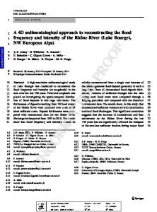
2.6.1. Site description A key difficulty with this part of the analysis was determining appropriate soil hydraulic parameters. These parameters are difficult to measure both in the laboratory and in the field. Previous studies have shown that soil hydraulic parameters under surface irrigation conditions exhibit poor correlation with soil texture and that pedotransfer functions have wide margins of errors when estimating these parameters (Selle et al., 2011; Zapata and Playán, 2000). Therefore, Zapata and Playán (2000) recommended fitting irrigation models to irrigation data as a mechanism for determining these parameters. The experimental data were collected with the purpose of conducting fertigation simulation studies, but were not intended to be used in combination with physically based infiltration models. As a result, the data set includes only pre-irrigation gravimetric water contents and an average soil texture (33% sand, 32% silt, and 35% clay). The soil particle size distribution is consistent with one of the soils found in the area, Kofa clay loam (Clayey over sandy, smectitic over mixed, calcareous, hyperthermic Typic Torrifluvents, [Hendricks, 1985]) as described by the USDA-NRCS Web Soil Survey. This particle size distribution was provided to the Rosetta pedotransfer module (Schaap et al., 2001) of HYDRUS-2D to estimate a set of soil hydraulic parameters. However, these parameters produced less than satisfactory irrigation simulation results. A better set of parameters was found using a different soil found in the area, Holtville clay (clayey over loamy, smectitic over mixed, superactive, calcareous, hyperthermic Typic Torrifluvents [Hendricks, 1985]). For this soil (sand = 12%, silt = 32%, clay = 56%), Rosetta estimated a higher value of the saturated water content, which was more consistent with the measured pre-irrigation water contents, and also a higher value of the saturated hydraulic conductivity, consistent with the value reported by the Web Soil Survey. These parameters are shown in Table 3. The residual water content, α, and n computed for the Kofa clay were not very different from those shown in the table. The 182.88 m long furrow had a blocked downstream end and on average zero slope, which increases the numerical complexity compared to a constant slope scenario. In particular, the slope varies between −0.0007 and 0.0007 (–) (Fig. 4). This is one of the reasons why this particular data set was chosen for the experimental model validation. A constant inflow rate of about 3.2 l/s for 44 min was used to irrigate the furrow, which was simultaneously fertigated with a bromide tracer. The solute was diluted in a separate tank, resulting in a concentration of approximately 40 g/l, and injected in the furrow with a constant flow rate of approximately 0.014 l/s. The solute tank emptied in about 37.5 min. Five measuring stations (grey dots in Fig. 4) were used to monitor the water level and solute distribution along the furrow length. Water levels and concentrations were measured

with an acquisition frequency of about 5 min. Soil water contents were measured gravimetrically before the irrigation at five measuring stations. The average volumetric water content was 0.35 cm3⁠ /cm3⁠ . A Manning’s coefficient of 0.04 s/m1⁠ /3 was used as suggested by USDA-NRCS (2012). Subsequent comparisons of measured with simulated flow depth hydrographs show that this is a reasonable roughness value. The geometric characteristics, soil hydraulic properties, and other input parameters are summarized in Table 2.

PR OO F

In the present study, the proposed hybrid FV-FE fertigation model is further experimentally validated against field data measured in 2001 at the Yuma Valley Agricultural Center, Yuma AZ, USA (C. Sanchez, 2018, personal communication).

3. Results and discussion 3.1. Theoretical validation 3.1.1. Mesh sensitivity analysis Fig. 5 shows water (top left plot) and solute (bottom left plot) profiles in the furrow at time t = 0.17 h (about 10 min) simulated with different mesh sizes dx. The advance curves (bottom right plot) and associated computational time (top right plot) are also shown in Fig. 5. At the first inspection, it is evident that the mesh size dx does not dramatically affect the numerical accuracy of the proposed model, which exhibits no overshooting and only limited numerical diffusion even for a coarse spatial discretization (i.e., dx = 10 m). Water and solute profiles for different dx are relatively close to each other. This is also true for the simulated advance curves, which deviate only at early times. However, as expected, false numerical diffusion increases with the mesh size. For dx = 10 m, the water profile was slightly smeared, and a faster waterfront advance was predicted for the first 60 m of the furrow length, as indicated by the red line in the bottom right plot of Fig. 5. This effect is more pronounced for the simulated solute profile, which clearly shows how the waterfront is ahead compared to what is calculated with dx = 2 or 5 m. This behavior is typical of FV models when the spatial discretization is coarse. False numerical diffusion tends to vanish when the mesh is refined, as demonstrated by the water and solute profiles as well as the advance curves for dx = 2 and 5 m, which almost overlap. This indicates that further mesh refinement will not increase the overall accuracy of the numerical solution, only the computational effort. Interest

Fig. 4. Geometric characteristics of the furrow located in Holtville (CA) that were used for experimental validation.

G. Brunetti et al.


Table 2 Geometric characteristics, soil hydraulic properties, and other input parameters used in experimental validation. Holtville 182.88 16 52 55 107 1.2 15 −0.0007 to 0.0007 (Variable) 0.04 0.35 3.2 0.014 40 0.5 0.1 44 37.5

PR OO F

Furrow length, L (m) Bottom width, bw⁠ (cm) Top width, Tw⁠ (cm) Ridge width, Rw⁠ (cm) Furrow spacing, FS (cm) Side slope, SS (–) Maximum depth, hm ⁠ ax (cm) Bed slope, S0⁠ (–) Manning’s coefficient, m (s/m1⁠ /3) Initial water content, θ0⁠ (–) Inflow rate, Qi⁠ r (l/s) Solute injection rate, Qi⁠ nj (l/s) Inflow concentration, Ci⁠ nj (g/l) Longitudinal dispersivity (cm), DL⁠ Transverse dispersivity (cm), DT⁠ Irrigation cutoff time, tw⁠ (min) Solute cutoff time, ts⁠ (min)

0.1

UN CO RR EC TE D

Table 3 The VGM hydraulic parameters used in experimental validation. θr⁠ (cm3⁠ /cm3⁠ )

is worth noting that the time step dt mainly influences the computation of the infiltration vector I, which is temporally discretized using the forward Euler approximation. More specifically, it is assumed that the nodal infiltration rate is constant during dt, which is an approximation wherein the accuracy depends on the variability of the infiltration rate during a particular time step. In this regard, the Horton’s infiltration theory (Horton, 1933) states that the infiltration rate into an initially dry soil typically decreases with time until reaching a steady-state value. Thus, when the soil is dry and the water level is small (i.e., the beginning of furrow irrigation), the infiltration rate declines rapidly and a fine time step is needed to accurately track infiltration. Thus, the stiffness of the infiltration term is appreciable at the beginning of the simulation when the furrow is dry, and the water level is relatively low. Under such circumstances, the vector I makes Eq. (1) moderately stiff. However, this effect is limited only to the first part of the simulation and tends to vanish when the water level rises and the soil saturates, as shown in Fig. 6. This analysis makes clear that the explicit approximation of the infiltration term is acceptable, provided that the time step dt is sufficiently small. Rather than using a constant time step, an adaptive time stepping discretization of the infiltration vector would likely increase the computational efficiency of the model while maintaining a good accuracy. The time step sensitivity analysis reveals that the computational cost is more influenced by the mesh size dx than by the time step dt. Indeed, the execution time only triples when dt = 30 s compared to when dt = 10 s. Overall, a time step dt = 20 s provides a good balance between the accuracy and computational cost. As a result of this analysis, a number of conclusions can be drawn:

θs⁠ (cm3⁠ /cm3⁠ )

α (1/ cm)

n (–)

Ks⁠ (cm/ min)

l (–)

0.5

0.017

1.26

0.017

0.5

ingly, the computational time increases almost linearly with dx. In particular, the execution time for dx = 2 m was 5.5 times greater than for dx = 10 m, while a mesh size dx = 5 m reduced the execution time by almost one third in comparison dx = 2 m. As a result of this analysis, a number of conclusions can be drawn:

- The proposed hybrid FV-FE model maintains a good accuracy even when a coarse mesh is adopted, which demonstrates an overall robustness of the model. This is of practical importance since it indicates that a model with coarse spatial discretization can be confidently used for preliminary design purposes or intensive numerical analyses, which require running the model multiple times. A classic example would be the application of a model with coarse discretization as a lower fidelity surrogate model in the Bayesian optimization framework (Razavi et al., 2012). - The effect of false numerical diffusion, although limited, tends to vanish when the mesh is refined. Therefore, when the analysis requires a higher accuracy, a reasonable mesh refinement will increase the overall accuracy of the model. - A mesh size dx = 5 m offers a good trade-off between numerical accuracy and computational cost. Further mesh refinements (i.e., dx = 2 m) lead to minimal accuracy gains and a significant increase in the model execution time. 3.1.2. Time step sensitivity analysis The results of the time step sensitivity analysis are shown in Fig. 6. The graph shows the simulated water (top left plot) and solute (bottom left plot) profiles at time t = 0.17 h (about 10 min) for different time steps dt. The advance curves (bottom right plot) and associated computational cost (top right plot) are also shown in Fig. 6. It is evident that, compared to the results obtained for different mesh sizes, the model exhibits a lower sensitivity to the time step dt. Very similar water and solute profiles were computed for all tested time steps (Fig. 6). Likewise, the computed advance curves were in closer agreement, especially at later times. Furthermore, the execution time increased linearly with the time step. It

- The time step dt has a small influence on the proposed hybrid FV-FE model in the analyzed range of time steps, reflecting a good robustness of the model. However, a time step sensitivity analysis is recommended to investigate the stiffness of the infiltration term, which increases for dry conditions and highly permeable soils. - An adaptive temporal discretization of the infiltration term in Eq. (1) would simultaneously increase the numerical accuracy and computational efficiency. This strategy should consist of small time steps in regions characterized by high infiltration gradients (i.e., dry soils) and larger time steps at later times when infiltration stabilizes (i.e., wet soils). Alternatively, future developments could also include the use of a correction factor that initially adjusts the infiltration rate and vanishes with time. This could be practically implemented in the present modeling framework using a scaling factor for the saturated hydraulic conductivity on the border of the furrow channel. - A time step dt = 20 s represents a good trade-off between the numerical accuracy and computational cost.

3.1.3. Validation scenarios Based on the results of the sensitivity analyses, the mesh size dx and the time step dt are set to 5 m and 20 s, respectively. Results of the theoretical validation are reported in Fig. 7. In particular, Fig. 7 shows a comparison between simulated advance curves, and water and solute profiles calculated by WinSRFR (dashed lines) and by the hybrid FV-FE model (solid lines) for the open end (top plots) and blocked end (bottom plots) scenarios. At the first inspection, it is evident that the results calculated by the proposed model matched very closely those computed with WinSRFR for both scenarios. More specifically, the advance curves nearly overlapped (right plots in Fig. 7) as did the rising branches of the water profiles (left plots in Fig. 7). However, the hydrographs deviated slightly from each other during the storage and recession phase. This effect is more evident for the blocked-end scenario, for which WinSRFR predicts a faster recession compared to the hybrid FE-FV model. This behavior is likely explained by the adoption of the explicit infiltration function of Warrick et al. (2007) in WinSRFR. When Warrick et al. (2007) first presented their explicit formulation, they compared the calculated cumulative infiltration for a rectangular channel against HYDRUS-2D. In particular, two soils were analyzed in that study: loam and sandy loam. In both cases, the explicit function showed a slight overestimation of cumulative infiltration, which


UN CO RR EC TE D

PR OO F

G. Brunetti et al.

Fig. 5. Simulation results for different mesh sizes dx: Water depth profiles at time t = 0.17 h (top left); surface solute profiles at time t = 0.17 h (bottom left); execution time (top right), and advance time with distance (bottom right).

is the same behavior encountered in the present study. Furthermore, Warrick et al. (2007) demonstrated that the edge effect increases with the water level and that it is more pronounced for parabolic and triangular channels than for rectangular channels. Thus, the overestimation of infiltration is expected to be substantial for trapezoidal channels, like the one analyzed in the present theoretical validation. Overall, the theoretical validation suggests that the proposed hybrid FE-FV model accurately describes the advance, storage, and depletion phase, as well as the solute transport during furrow irrigation and fertigation. Furthermore, the analysis reveals that the model is oscillation-free in the analyzed cases and stable for a variety of boundary conditions, thus it can be confidently used for analyzing real systems. Nevertheless, it must be emphasized that the analyzed scenarios are not exhaustive of all practical modeling situations, therefore we plan to make the model open source and available to users in order to receive continuous feedback and validation.

depth profiles (upper graphs) and advance curves (bottom graphs). All field measurements were reasonably well predicted by the model. Differences between water levels at x = 4.57 m (Fig. 8) can be attributed to furrow survey errors. Nevertheless, the general trend highlights good model performances. This is confirmed by the model’s ability to accurately reproduce measured concentration breakthrough curves. Although the solute concentration data are noisy, both the time arrival of the solute plume and the peak concentrations are predicted accurately. The solute dilution at x = 4.57 and 45.72 m induced by solute cutoff is well simulated by the model, thus indicating a good reliability of the proposed numerical approach. The advance curve (Fig. 9) is generally reproduced with high accuracy, except at x = 137.16 m where the model predicts a delay in the advance of the waterfront (Fig. 9). This is confirmed by a slight underestimation (i.e., ≈1 cm) of the water depth at x = 137.16 m (top plot in Fig. 9), which, however, tends to disappear with time. In our opinion, these small deviations are mainly due to slope uncertainties and the spatial variability of soil hydraulic properties. Water profiles (top plot in Fig. 9) are very well approximated, except for a small underestimation in the first part of the furrow. Interestingly, this behavior is not systematic but limited to particular simulation times (i.e., t = 42–82 min), likely reflecting small measurement errors.

3.2. Experimental validation

Figs. 8 and 9 compare modeling results (solid lines) with experimental results (circles). The first figure (Fig. 8) depicts hydrographs (left graphs) and concentration breakthrough curves (right graphs), while Fig. 9 displays water 11


UN CO RR EC TE D

PR OO F

G. Brunetti et al.

Fig. 6. Simulation results for different time steps dt: Water depth profiles at time t = 0.17 h (top left); surface solute profiles at time t = 0.17 h (bottom left); execution time (top right); advance time with distance (bottom right).

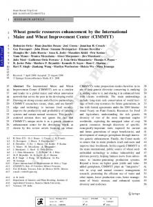
It must be emphasized that soil hydraulic parameters used in the simulation were generated using the ROSETTA pedotransfer model, predictions of which for the saturated values can be affected by high uncertainties (Rubio et al., 2008). The bias associated with the estimation of Ks⁠ can, therefore, partially explain the model deviations. Better estimations of soil hydraulic parameters could be obtained by comparing simulated and measured subsurface quantities (e.g., water contents or pressure heads). Thus, a complete dataset, which includes information about both surface and subsurface domains, is recommended for a comprehensive model calibration and an assessment of its uncertainty. Further plausible sources of uncertainties are related to the assumption of constant initial conditions and to the adopted value of the Manning’s coefficient. Indeed, the bias in the simulated water level at x = 137.16 m could be potentially explained by the underestimation of the near-surface water content at the beginning of the infiltration. Similarly, the delay in the simulated advance curve could be attributed to the assumption of the roughness homogeneity along the furrow. One of the key advantages of the proposed hybrid FE-FV model is its ability to provide a mechanistic description of the transport processes in the subsurface domain. Fig. 10 shows the simulated post-irrigation (t = 7.7 h) distribution of water contents (left plots) and solute concentrations (right plots) in the soil at different measuring stations. Differences in the water content are mostly

explained by slight variations in field elevations – high points in the field infiltrated less water than low points. Note that the wetting bulbs of neighboring furrows did not merge and that a considerable amount of water was stored below the furrow bed. Conventional furrow irrigation models ignore the non-uniform distribution of water in a furrow cross section and instead assume a uniform water distribution. Clearly, this distribution needs to be accounted for in order to properly evaluate the irrigation performance (e.g., distribution uniformity, application efficiency, requirement efficiency). On the other hand, the moisture distribution along the furrow was homogeneous. Such a uniform longitudinal distribution can be expected with zero-slope irrigation systems, as differences in opportunity time along the field are small. On the other hand, a very different situation occurs for fertigation. The solute distribution differs from the water distribution. Solute mostly accumulates between x = 91.44 m and x = 137.16 m, while it is unevenly distributed in remaining parts of the furrow. This behavior is particularly exacerbated for x < 91.44 m, where recession times occur earlier than in the remainder of the furrow. In such circumstances, plants located in the first part of the furrow will receive less fertilizer, leading to an unbalanced crop production. The analysis reveals that the unevenness of the furrow bottom slope negatively affects the uniformity of solute distribution. However, it must be emphasized that the available dataset did not include measurements of water contents and solute

12


PR OO F

G. Brunetti et al.

UN CO RR EC TE D

Fig. 7. Simulated water (left) and solute (middle) hydrographs, and advance curves (right) calculated using WinSRFR (dashed lines) and hybrid FV-FE (solid lines) models for the open end (top plots) and blocked end (bottom plots) scenarios.

concentrations in the soil profile and thus it was not possible to validate simulated soil water contents and solute concentrations in the soil. Results demonstrate the usefulness of the proposed modeling approach and its ability to account for the solute and moisture distributions along the entire furrow. In the future, these results could be interestingly used as initial conditions for daily or weekly numerical simulations with HYDRUS-2D to identify crop stresses and to optimize the irrigation schedule.

tivity analysis is used to examine the effects of the coarse spatial discretization on the results of the model. The analysis reveals that the model guarantees a sufficient accuracy even for larger mesh sizes, thus suggesting its application as a lower fidelity surrogate in computationally intensive statistical analyses (e.g., Brunetti et al., 2017a, 2017b). To increase the computational efficiency of the proposed numerical framework, the infiltration component is explicitly linearized in time, thus avoiding the iterative execution of HYDRUS at each time step. The validity of this assumption is confirmed by a preliminary time sensitivity analysis, which confirms the robustness of the developed model and clarifies how the stiffness of the infiltration term decreases with time. In this light, future work should investigate the use of adaptive time stepping strategies for the evaluation of infiltration. Theoretical and experimental validations demonstrate the accuracy of the proposed hybrid FV-FV furrow irrigation and fertigation model, which is able to provide a mechanistic description of the water and solute distribution in the soil along the furrow. Hence, future applications and developments should focus on the use and testing of the proposed model for the numerical investigation of the root solute and water uptake of typical crops in long-term simulation scenarios.

4. Conclusions and summary

The main objective of this study was to develop a numerical model able to provide an accurate mechanistic description of the coupled surface-subsurface processes happening during furrow irrigation and fertigation. The proposed modeling framework combines a one-dimensional description of water flow and solute transport in the surface domain, based on the Zero-Inertia approximation of the hydrodynamic wave and the advection equation for solute transport, respectively, with a two-dimensional description of water flow and solute transport in the subsurface domain, based on the Richards and advection-dispersion equations, respectively. One of the main novelties of this study is the implementation in the coupled model of the widely used Finite Element model, HYDRUS, which can describe the simultaneous movement of water, heat, and solutes in porous media and which can provide a basis for analyzing many different scenarios and conditions. The surface domain is solved using the Method of Lines in conjunction with a high-order MUSCL Finite Volume scheme combined with the well-established Dormand-Prince (RKDP) temporal discretization method, thus leading to a hybrid FV-FE furrow irrigation and fertigation model. The mesh sensi

Acknowledgements We thank Dr. Charles Sanchez from University of Arizona (US) for kindly providing us experimental data used in model validation and Dr. Honeyeh Kazemi for organizing the experimental data.

13


UN CO RR EC TE D

PR OO F

G. Brunetti et al.

Fig. 8. Modeled (red lines) and measured (grey dots) hydrographs (plots in the third column) and concentration breakthrough curves (plots in fourth column), and against each other (plots in the first and second column) at different furrow locations (rows from top down for x = 4.57, 45.72, 91.44, 137.16, and 180.74 m) for the Holtville validation scenario. The dashed black lines indicate the regression lines. (For interpretation of the references to colour in this figure legend, the reader is referred to the web version of this article.)

14


UN CO RR EC TE D

PR OO F

G. Brunetti et al.

Fig. 9. Modeled (solid lines) and measured (dots) water profiles (top plot) and advance curves (bottom plot) for the Holtville validation scenario.

15

G. Brunetti et al.


UN CO RR EC TE D

PR OO F

Brufau, P., Garcia-Navarro, P., Playán, E., Zapata, N., 2002. Numerical modeling of basin irrigation with an upwind scheme. J. Irrig. Drain. Eng. 128, 212–223. https://doi.org/ 10.1061/(asce)0733-9437(2002) 128:4(212). Brunetti, G., Saito, H., Saito, T., Šimůnek, J., 2017. A computationally efficient pseudo-3D model for the numerical analysis of borehole heat exchangers. Appl. Energyhttps:// doi.org/10.1016/j.apenergy.2017.09.042. Brunetti, G., Šimůnek, J., Turco, M., Piro, P., 2017. On the use of surrogate-based modeling for the numerical analysis of Low Impact Development techniques. J. Hydrol. 548, 263–277. https://doi.org/10.1016/j.jhydrol.2017.03.013. Burguete, J., Zapata, N., García-Navarro, P., Maïkaka, M., Playán, E., Murillo, J., 2009. Fertigation in furrows and level furrow systems. I: model description and numerical tests. J. Irrig. Drain. Eng. 135, 401–412. https://doi.org/10.1061/(ASCE)IR.1943-4774. 0000097. Carsel, R.F., Parrish, R.S., 1988. Developing joint probability distributions of soil water retention characteristics. Water Resour. Res. 24, 755–769. https://doi.org/10.1029/ WR024i005p00755. Dong, Q., Xu, D., Zhang, S., Bai, M., Li, Y., 2013. A hybrid coupled model of surface and subsurface flow for surface irrigation. J. Hydrol. 500, 62–74. https://doi.org/10. 1016/j.jhydrol.2013.07.018. Dormand, J.R., Prince, P.J., 1980. A family of embedded Runge-Kutta formulae. J. Comput. Appl. Math. 6, 19–26. https://doi.org/10.1016/0771-050X(80)90013-3. Ebrahimian, H., Keshavarz, M.R., Playán, E., 2014. Surface fertigation: A review, gaps and needs. Span. J. Agric. Res. http://doi.org/10.5424/sjar/2014123-5393. Ebrahimian, H., Liaghat, A., Parsinejad, M., Playán, E., Abbasi, F., Navabian, M., 2013. Simulation of 1D surface and 2D subsurface water flow and nitrate transport in alternate and conventional furrow fertigation. Irrig. Sci. 31, 301–316. https://doi.org/10. 1007/s00271-011-0303-3. Fahong, W., Xuqing, W., Sayre, K., 2004. Comparison of conventional, flood irrigated, flat planting with furrow irrigated, raised bed planting for winter wheat in China. Field Crops Res. 87, 35–42. https://doi.org/10.1016/j.fcr.2003.09.003. FAO, 2011a. The State of the World’s land and water resources for Food and Agriculture. Managing systems at risk, Food and Agriculture Organization. ISBN:978-1-84971-326-9. FAO, 2011b. Irrigation in Southern and Eastern Asia in figures, AQUASTAT Survey – FAO Water report 37. ISBN:978-92-5-107282-0. FAO, 2015. World fertilizer trends and outlook to 2018, Food and Agriculture Organization of United Nations. FAO, 2017. The future of food and agriculture – Trends and challenges. Rome. Furman, A., 2008. Modeling Coupled Surface-Subsurface Flow Processes: A Review. Vadose Zo. J. 7, 741–756. https://doi.org/10.2136/vzj2007.0065. Godunov, S.K., Moscow, S.U., 1954. Ph. D. Dissertation: Difference Methods for Shock Waves. Moscow State University. He, Z., Wu, W., Wang, S.S., 2008. Coupled Finite-Volume Model for 2D Surface and 3D Subsurface Flows. J. Hydrol. Eng. 13, 835–845. https://doi.org/10.1061/ (ASCE)1084-0699(2008) 13:9(835). Hendricks, D.M., 1985. Arizona Soils. College of Agriculture, University of Arizona. Horst, M.G., Shamutalov, S.S., Pereira, L.S., Gonçalves, J.M., 2005. Field assessment of the water saving potential with furrow irrigation in Fergana, Aral Sea basin. Agric. Water Manage. 77, 210–231. https://doi.org/10.1016/j.agwat.2004.09.041. Horton, R.E., 1933. The role of infiltration in the hydrologic cycle. Trans. Am. Geophys. Union 445–460, https://doi.org/10.1029/TR014i001p00446. Katopodes, N.D., Strelkoff, T.S., 1977. Dimensionless solutions of border-irrigation advance. J. Irrig. Drain. Eng. 103, 401–417. Lal, A.M.W., 1998. Weighted implicit finite-volume model for overland flow. J. Hydraul. Eng. 124, 941–950. https://doi.org/10.1061/(ASCE)0733-9429(1998) 124:9(941). Lazarovitch, N., Warrick, A.W., Furman, A., Zerihun, D., 2009. Subsurface water distribution from furrows described by moment analyses. J. Irrig. Drain. Eng. 135, 7–12. https://doi.org/10.1061/(ASCE)0733-9437(2009) 135:1(7). LeVeque, R.J., 2002. Finite Volume Methods for Hyperbolic Problems, vol. 54. Cambridge Univ. Press, p. 258. http://doi.org/10.1017/CBO9780511791253. Oweis, T.Y., Walker, W.R., 1990. Zero-inertia model for surge flow furrow irrigation. Irrig. Sci. 11, 131–136. https://doi.org/10.1007/BF00189449. Perea, H., Strelkoff, T.S., Adamsen, F.J., Hunsaker, D.J., Clemmens, A.J., 2010. Nonuniform and unsteady solute transport in furrow irrigation. I: model development. J. Irrig. Drain. Eng. 136, 365–375. https://doi.org/10.1061/(ASCE)IR.1943-4774.0000106. Razavi, S., Tolson, B.A., Burn, D.H., 2012. Review of surrogate modeling in water resources. Water Resour. Res. 48, n/a-n/a. http://doi.org/10.1029/2011WR011527. Rubio, C.M., Llorens, P., Gallart, F., 2008. Uncertainty and efficiency of pedotransfer functions for estimating water retention characteristics of soils. Eur. J. Soil Sci. 59, 339–347. https://doi.org/10.1111/j.1365-2389.2007.01002.x. Sargent, R.G., 1998. Verification and validation of simulation models. Simul. Conf. Proceedings, 1998. Winter 1, 121–130. http://doi.org/10.1109/WSC.1998.744907. Schaap, M.G., Leij, F.J., Van Genuchten, M.T., 2001. Rosetta: a computer program for estimating soil hydraulic parameters with hierarchical pedotransfer functions. J. Hydrol. 251, 163–176. https://doi.org/10.1016/S0022-1694(01)00466-8. Schlesinger, Crosby, R., Cagne, R., Innis, G., Lalwani, C., Loch, J., Sylvester, R., Wright, R., Kheir, N., Bartos, D., 1979. Terminology for model credibility. Simulation 32, 103–104. http://doi.org/10.1177/003754977903200304. Selle, B., Minasny, B., Bethune, M., Thayalakumaran, T., Chandra, S., 2011. Applicability of Richards’ equation models to predict deep percolation under surface irrigation. Geoderma 160, 569–578. https://doi.org/10.1016/J.GEODERMA.2010.11.005. Šimůnek, J., Bristow, K.L., Helalia, S.A., Siyal, A.A., 2016. The effect of different fertigation strategies and furrow surface treatments on plant water and nitrogen use. Irrig. Sci. 34, 53–69. https://doi.org/10.1007/s00271-015-0487-z. Šimůnek, J., van Genuchten, M.T., Šejna, M., 2016. Recent developments and applications of the HYDRUS computer software packages. Vadose Zo. J. 15, 25. https://doi.org/ 10.2136/vzj2016.04.0033.

Fig. 10. Simulated distributions of soil water contents (left plots) and solute concentrations (right plots) in the vertical 2D domains at different measuring stations.

References

Abbasi, F., Simunek, J., van Genuchten, M.T., Feyen, J., Adamsen, F.J., Hunsaker, D.J., Strelkoff, T.S., Shouse, P., 2003. Overland water flow and solute transport: model development and field-data analysis. J. Irrig. Drain. Eng. 129, 71–81. https://doi.org/ 10.1061/(ASCE)0733-9437(2003) 129:2(71). Bautista, E., Clemmens, A.J., Strelkoff, T.S., Schlegel, J., 2009. Modern analysis of surface irrigation systems with WinSRFR. Agric. Water Manage. 96, 1146–1154. https://doi. org/10.1016/j.agwat.2009.03.007. Bautista, E., Warrick, A.W., Schlegel, J.L., Thorp, K.R., Hunsaker, D.J., 2016. Approximate furrow infiltration model for time-variable ponding depth. J. Irrig. Drain. Eng. 142, 4016045. https://doi.org/10.1061/(ASCE)IR.1943-4774.0001057. Bautista, E., Warrick, A.W., Strelkoff, T.S., 2014. New results for an approximate method for calculating two-dimensional furrow infiltration. J. Irrig. Drain. Eng. 140, 4014032. https://doi.org/10.1061/(ASCE)IR.1943-4774.0000753. Beirami, M.K., Nabavi, S.V., Chamani, M.R., 2006. Free overfall in channels with different cross sections and sub-critical flow. Iran. J. Sci. Technol. Trans. B, Eng. 30. Bradford, S.F., Katopodes, N.D., 2001. Finite volume model for nonlevel basin irrigation. J. Irrig. Drain. Eng. 127, 216–223. https://doi.org/10.1061/(ASCE)0733-9437(2001) 127:4(216). Bradford, S.F., Sanders, B.F., 2002. Finite-volume model for shallow-water flooding of arbitrary topography. J. Hydraul. Eng. 128, 289–298. https://doi.org/10.1061/ (ASCE)0733-9429(2002) 128:3(289). Brent, R.P., 1974. Algorithms for minimization without derivatives. IEEE Trans. Automat. Contr. 19, 632–633. https://doi.org/10.1109/TAC.1974.1100629.

16

G. Brunetti et al.

Computers and Electronics in Agriculture xxx (2018) xxx-xxx van Leer, B., 1979. Towards the ultimate conservative difference scheme. V. A second-order sequel to Godunov’s method. J. Comput. Phys. 32, 101–136. https://doi.org/10. 1016/0021-9991(79)90145-1. Walker, W.R., Humpherys, A.S., 1983. Kinematic-wave furrow irrigation model. J. Irrig. Drain. Eng. 109, 377–392. https://doi.org/10.1061/(ASCE)0733-9437(1983) 109: 4(377). Warrick, A.W., Lazarovitch, N., Furman, A., Zerihun, D., 2007. Explicit infiltration function for furrows. j. Irrig. Drain. Eng. 133, 307–313. https://doi.org/10.1061/ (ASCE)0733-9437(2007) 133:4(307). Wöhling, T., Fröhner, A., Schmitz, G.H., Liedl, R., 2006. Efficient solution of the coupled one-dimensional surface—two-dimensional subsurface flow during furrow irrigation advance. J. Irrig. Drain. Eng. 132, 380–388. https://doi.org/10.1061/ (ASCE)0733-9437(2006) 132:4(380). Wöhling, T., Mailhol, J., 2007. Physically based coupled model for simulating 1D surface–2D subsurface flow and plant water uptake in irrigation furrows. II: Model test and evaluation. J. Irrig. Drain. Eng. 133, 548–558. https://doi.org/10.1061/ (ASCE)0733-9437(2007) 133:6(548). Wöhling, T., Schmitz, G.H., 2007. Physically based coupled model for simulating 1D surface–2D subsurface flow and plant water uptake in irrigation furrows. I: Model development. Irrig. Drain. Eng. 133, 538–547. https://doi.org/10.1061/ (ASCE)0733-9437(2007) 133:6(538). Wöhling, T., Singh, R., Schmitz, G.H., 2004. Physically based modeling of interacting surface-subsurface flow during furrow irrigation advance. J. Irrig. Drain. Eng. 130, 349–356. https://doi.org/10.1061/(ASCE)0733-9437(2004) 130:5(349). Zapata, N., Playán, E., 2000. Elevation and infiltration in a level basin. I. Characterizing variability. Irrig. Sci. 19, 155–164. https://doi.org/10.1007/s002710000017. Zerihun, D., Furman, A., Warrick, A.W., Sanchez, C.A., 2005. Coupled surface-subsurface flow model for improved basin irrigation management. J. Irrig. Drain. Eng. 131, 111–128. http://doi.org/10.1061/(ASCE)0733-9437(2005)131:2(111).

UN CO RR EC TE D

PR OO F

Siyal, A.A., Bristow, K.L., Šimůnek, J., 2012. Minimizing nitrogen leaching from furrow irrigation through novel fertilizer placement and soil surface management strategies. Agric. Water Manage. 115, 242–251. https://doi.org/10.1016/j.agwat.2012.09.008. Soroush, F., Fenton, J.D., Mostafazadeh-Fard, B., Mousavi, S.F., Abbasi, F., 2013. Simulation of furrow irrigation using the Slow-change/slow-flow equation. Agric. Water Manage. 116, 160–174. https://doi.org/10.1016/j.agwat.2012.07.008. Strelkoff, T.S., Clemmens, A.J., Perea-Estrada, H., 2006. Calculation of non-reactive chemical distribution in surface fertigation. Agric. Water Manage. 86, 93–101. https://doi. org/10.1016/j.agwat.2006.07.006. Strelkoff, T.S., Katopodes, N.D., 1977. Border-irrigation hydraulics with zero inertia. J. Irrig. Drain. Eng. 103, 325–342. Tabuada, M.A., Rego, Z.J.C., Vachaud, G., Pereira, L.S., 1995. Modelling of furrow irrigation. Advance with two-dimensional infiltration. Agric. Water Manage. 28, 201–221. https://doi.org/10.1016/0378-3774(95)01177-K. USDA-NRCS, 2012. Surface irrigation. In: National Engineering Handbook. van Genuchten, M.T., 1976. On the accuracy and efficiency of several numerical schemes for solving the convective-dispersive equation. In: Gray, W. (Ed.), Finite Elements in Water Resources. Pentech Press, London, pp. 1.71–1.90. van Genuchten, M.T., 1978. Mass transport in saturated-unsaturated media: one-dimensional solutions, in: Research Rep. No. 78-WR-11. University, Princeton, Princeton. van Genuchten, M.T., 1980. A closed-form equation for predicting the hydraulic conductivity of unsaturated soils1. Soil Sci. Soc. Am. J. 44, 892–898. https://doi.org/10. 2136/sssaj1980.03615995004400050002x. van Leer, B., 1974. Towards the ultimate conservative difference scheme. II. Monotonicity and conservation combined in a second-order scheme. J. Comput. Phys. 14, 361–370. https://doi.org/10.1016/0021-9991(74)90019-9.

17