Jun 1, 2008 - ... next integer time. Figure 1b shows another allowed collision, in which .... don't have to worry about synchronizing signalsâ they all remain in ...
arXiv:0806.0127v1 [nlin.CG] 1 Jun 2008
Universal Cellular Automata Based on the Collisions of Soft Spheres∗ Norman Margolus
Abstract
the information density and processing rate in a CA dynamics is also physically realistic. These connecFredkin’s Billiard Ball Model (BBM) is a continuous tions with physics have been exploited to construct classical mechanical model of computation based on CA models of spatial processes in Nature and to the elastic collisions of identical finite-diameter hard explore artificial “toy” universes. The discrete and spheres. When the BBM is initialized appropriately, uniform spatial structure of CA computations also the sequence of states that appear at successive integer makes it possible to “crystallize” them into efficient time-steps is equivalent to a discrete digital dynamics. hardware[19, 21]. Here we discuss some models of computation that Here we will focus on CA’s as realistic spatial modare based on the elastic collisions of identical finiteels of ordinary (non-quantum-coherent) computation. diameter soft spheres: spheres which are very comAs Fredkin and Banks pointed out[3], we can demonpressible and hence take an appreciable amount of strate the computing capability of a CA dynamics time to bounce off each other. Because of this by showing that certain patterns of bits act like logic extended impact period, these Soft Sphere Models gates, like signals, and like wires, and that we can (SSM’s) correspond directly to simple lattice gas put these pieces together into an initial state that, automata—unlike the fast-impact BBM. Successive under the dynamics, exactly simulates the logic cirtime-steps of an SSM lattice gas dynamics can be cuitry of an ordinary computer. Such a CA dynamviewed as integer-time snapshots of a continuous ics is said to be computation universal. A CA may physical dynamics with a finite-range soft-potential also be universal by being able to simulate the operinteraction. We present both 2D and 3D models ation of a computer in a less efficient manner—never of universal CA’s of this type, and then discuss reusing any logic gates for example. A universal CA spatially-efficient computation using momentum conthat can perform long iterative computations within serving versions of these models (i.e., without fixed a fixed volume of space is said to be a spatially effimirrors). Finally, we discuss the interpretation of cient model of computation. these models as relativistic and as semi-classical sysWe would like our CA models of computation to tems, and extensions of these models motivated by be as realistic as possible. They should accurately these interpretations. reflect important constraints on physical information processing. For this reason, one of the ba1 Introduction sic properties that we incorporate into our models is the microscopic reversibility of physical dynamCellular Automata (CA) are spatial computations. ics: there is always enough information in the miThey imitate the locality and uniformity of physical croscopic state of a physical system to determine law in a stylized digital format. The finiteness of not only what it will do next, but also exactly what ∗ This is a posting to arXiv.org of a paper that was originally state it was in a moment ago. This means, in parpublished in 2002 as a chapter of a book [22]. ticular, that in reversible CA’s (as in physics) we 1
can never truly erase any information. This constraint, combined with energy conservation, allows reversible CA systems to accurately model thermodynamic limits on computation[4, 9]. Conversely, reversible CA’s are particularly useful for modeling thermodynamic processes in physics[5]. Reversible CA “toy universes” also tend to have long and interesting evolutions[19, 6]. All of the CA’s discussed in this paper fall into a class of CA’s called Lattice Gas Automata (LGA), or simply lattice gases. These CA’s are particularly well suited to physical modeling. It is very easy to incorporate constraints such as reversibility, energy conservation and momentum conservation into a lattice gas. Lattice gases are known which, in their largescale average behavior, reproduce the normal continuum differential equations of hydrodynamics[14, 13]. In a lattice gas, particles hop around from lattice site to lattice site. These models are of particular interest here because one can imagine that the particles move continuously between lattice sites in between the discrete CA time-steps. Using LGA’s allows us to add energy and momentum conservation to our computational models, and also to make a direct connection with continuous classical mechanics. Our discussion begins with the most realistic classical mechanical model of digital computation, Fredkin’s Billiard Ball Model[11]. We then describe related classical mechanical models which, unlike the BBM, are isomorphic to simple lattice gases at integer times. In the BBM, computations are constructed out of the elastic collisions of very incompressible spheres. Our new 2D and 3D models are based on elastically colliding spheres that are instead very compressible, and hence take an appreciable amount of time to bounce off each other. The universality of these Soft Sphere Models (SSM’s) depends on the finite extent in time of the interaction, rather than its finite extent in space (as in the BBM). This difference allows us to interpret these models as simple LGA’s. Using the SSM’s, we discuss computation in perfectly momentum conserving physical systems (cf. [24]), and show that we can compute just as efficiently in the face of this added constraint. The main difficulty here turns out to be reusing signal-routing resources. We then provide an alternative physical
interpretation of the SSM’s (and of all mass and momentum conserving LGA’s) as relativistic systems, and discuss some alternative relativistic SSM models. Finally, we discuss the use of these kinds of models as semi-classical systems which embody realistic quantum limits on classical computation.
2
Fredkin’s Billiard Ball Model
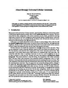
In Figure 1, we summarize Edward Fredkin’s classical mechanical model of computation, the Billiard Ball Model. His basic insight is that a location where balls may or may not collide acts like a logic gate: we get a ball coming out at certain places only if another ball didn’t knock it away! If the balls are used as signals, with the presence of a ball representing a logical “1” and the absence a logical “0”, then a place where signals intersect acts as a logic gate, with different logic functions of the inputs coming out at different places. Figure 1a illustrates the idea in more detail. For this to work right, we need synchronized streams of data, with evenly spaced time-slots in which a 1 (ball) or 0 (no ball) may appear. When two 1’s impinge on the collision “gate”, they behave as shown in the Figure, and they come out along the paths labeled AB. If a 1 comes in at A but the corresponding slot at B is empty, then that 1 makes it through to the path la¯ (A and not B). If sequences of such gates beled AB can be connected together with appropriate delays, the set of logic functions that appear at the outputs in Figure 1a is sufficient to build any computer. In order to guarantee composability of these logic gates, we constrain the initial state of the system. All balls are identical and are started at integer coordinates, with the unit of distance taken to be the diameter of the balls. This spacing is indicated in the Figure by showing balls centered in the squares of a grid. All balls move at the same speed in one of four directions: up-right, up-left, down-right, or down-left. The unit of time is chosen so that at integer times, all freely moving balls are again found at integer coordinates. We arrange things so that balls always collide at right angles, as in Figure 1a. Such a collision leaves the colliding balls on the grid at the next integer time. Figure 1b shows another allowed collision, in which 2
AB
A
A
A
AB
AB
A
B
B
A
AB
B
(a)
AB
AB
AB
AB
B
A
(b)
(c)
(d)
Figure 1: The Billiard Ball Model. Balls are always found at integer coordinates at integer times. (a) A collision that does logic. Two balls are initially moving towards each other to the right. Successive columns catch the balls at successive integer times. The dotted lines indicate paths the balls would have taken if only one or the other had come in (i.e., no collision). (b) Balls can collide at half-integer times (gray). (c) Billiard balls are routed and delayed by carefully placed mirrors as needed to connect logic-gate collisions together. Collisions with mirrors can occur at either integer or half-integer times. (d) Using mirrors, we can make two signal paths cross as if the signals pass right through each other. the balls collide at half-integer times (shown in gray) but are still found on the grid at integer times. The signals leaving one collision-gate are routed to other gates using fixed mirrors, as shown in Figure 1c. The mirrors are strategically placed so that balls are always found on the grid at integer times. Since zeros are represented by no balls (i.e., gaps in streams of balls), zeros are routed just as effectively by mirrors as the balls themselves are. Finally, in Figure 1d, we show how two signal streams are made to cross without interacting—this is needed to allow wires to cross in our logic diagrams. In the collision shown, if two balls come in, one each at A and B, then two balls come out on the same paths and with the same timing as they would have if they had simply passed straight through. Needless to say, if one of the input paths has no ball, a ball on the other path just goes straight through. And if both inputs have no ball, we will certainly not get any balls at the outputs, so the zeros go straight through as well.
and collide or not at each intersection, exactly as they did going forward. Even if we don’t actually reverse the velocities, we know that there is enough information in the present state to recover any earlier state, simply because we could reverse the dynamics. Thus we have a classical mechanical system which, viewed at integer time steps, performs a discrete reversible digital process.
The digital character of this model depends on more than just starting all balls at integer coordinates. We need to be careful, for example, not to wire two outputs together. This would result in head-on collisions which would not leave the balls on the grid at integer times! Miswired logic circuits, in which we use a collision gate backward with the four inputs improperly correlated, would also spoil the digital character of the model. Rather than depending on correct logic design to assure the applicability of the digital interpretation, we can imagine that our balls have an interaction potential that causes them to pass Clearly any computation that is done using the through each other without interacting in all cases BBM is reversible, since if we were to simultaneously that would cause problems. This is a bit strange, and exactly reverse the velocities of all balls, they but it does conserve energy and momentum and is would exactly retrace their paths, and either meet reversible. Up to four balls, one traveling in each di3
3
rection, can then occupy the same grid cell as they pass through each other. We can also associate the mirror information with the grid cells, thus completing the BBM as a CA model. Unfortunately this is a rather complicated CA with a rather large neighborhood. The complexity of the BBM as a CA rule can be attributed to the non-locality of the hard-sphere interaction. Although the BBM interaction can be softened—with the grid correspondingly adjusted— this model depends fundamentally upon information interacting at a finite distance. A very simple CA model based on the BBM, the BBMCA[15, 19] avoids this non-locality by modeling the front and back edges of each ball, and using a sequence of interactions between edge-particles to simulate a billiard ball collision. This results in a reversible CA with just a 4-bit neighborhood (including all mirror information!), but this model gives up exact momentum conservation, even in simulating the collision of two billiard balls. In addition to making the BBMCA less physical, this loss of conservation makes BBMCA logic circuits harder to synchronize than the original BBM. In the BBM, if we start a column of signals out, all moving up-right or down-right, then they all have the same horizontal component of momentum. If all the mirrors they encounter are horizontal mirrors, this component remains invariant as we pass the signals through any desired sequence of collision “gates.” We don’t have to worry about synchronizing signals— they all remain in a single column moving uniformly to the right. In the BBMCA, in contrast, simulated balls are delayed whenever they collide with anything. In a BBMCA circuit with only horizontal mirrors (or even without any mirrors), the horizontal component of momentum is not conserved, the center of mass does not move with constant horizontal velocity, and appropriate delays must be inserted in order to bring together signals that have gotten out of step. The BBMCA has energy conservation, but not momentum conservation. It turns out that it is easy to make a model which is very similar to the BBM, which has the same kind of momentum conservation as the BBM, and which corresponds isomorphically to a simple CA rule.
A Soft Sphere Model
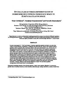
Suppose we set things up exactly as we did for the BBM, with balls on a grid, moving so that they stay on the grid, but we change the collision, making the balls very compressible. In Figure 2a, we illustrate the elastic collision of two balls in the resulting Soft Sphere Model (SSM). If the springiness of the balls is just right (i.e., we choose an appropriate interaction potential), then the balls find themselves back on the grid after the collision. If only one or the other ball comes in, they go straight through. Notice that the output paths are labeled exactly as in the BBM model, except that the AB paths are deflected inwards rather than outwards (cf. Appendix to [15]). If we add BBM-style hard-collisions with mirrors,1 then this model can compute in the same manner as the BBM, with the same kind of momentum conservation aiding synchronization. In Figure 2b, we have drawn an arrow in each grid cell corresponding to the velocity of the center of a ball at an integer time. The pair of colliding balls is taken to be a single particle, and we also draw an arrow at its center. We’ve colored the arrows alternately gray and black, corresponding to successive positions of an incoming pair of logic values. We can now interpret the arrows as describing the dynamics of a simple lattice gas, with the sites of the lattice taken to be the corners of the cells of the grid. In a lattice gas, we alternately move particles and let them interact. In this example, at each lattice site we have room for up to eight particles (1’s): we can have one particle moving up-right, one down-right, one up-left, one down-left, one right, one left, one up and one down. In the movement step, all up-right particles are simultaneously moved one site up and one site to the right, while all down-right particles are moved down and to the right, etc. After all particles have been moved, we let the particles that have landed at each lattice site interact—the interaction at each lattice site is independent of all other lattice sites. In the lattice gas pictured in Figure 2b, we see on 1 All of the 90◦ turns that we use in our SSM circuits can also be achieved by soft mirrors placed at slightly different locations.
4
AB
A
AB A
AB
AB
AB
B
AB
(a)
AB
B
A
AB
(b)
0
1
1
0
1
0
0
1
1
1
1
1
A
(c)
(d)
Figure 2: A soft sphere model of computation. (a) A BBM-like collision using very compressible balls. The springiness of the balls is chosen so that after the collision, the balls are again at integer sites at integer times. The logic is just like the BBM, but the paths are deflected inwards, rather than outwards. (b) Arrows show the velocities of balls at integer times. During the collision, we consider the pair to be a single mass, and draw a single arrow. (c) We can route and delay signals using mirrors. (d) We can make signals cross. state shown on the left turn into the same rotation of the state shown on the right. In all other cases, particles go straight. This is a simple reversible rule, and (except in the presence of mirrors) it exactly conserves momentum. We will discuss a version of this model later without mirrors, in which momentum is always conserved.
the left particles coming in on paths A and B that are entering two lattice sites (black arrows) and the resulting data that leaves those sites (gray arrows). Our inferred rule is that single diagonal particles that enter a lattice site come out in the same direction they came in. At the next step, these gray arrows represent two particles entering a single lattice site. Our inferred rule is that when two diagonal particles collide at right angles, they turn into a single particle moving in the direction of the net momentum. Now a horizontal black particle enters the next lattice site, and our rule is that it turns back into two diagonal particles. If only one particle had come in, along either A or B, it would have followed our “single diagonal particles go straight” rule, and so single particles would follow the dotted path in the figure. Thus our lattice gas exactly duplicates the behavior of the SSM at integer times.
The relationship between the SSM of Figure 2a and a lattice gas can also be obtained by simply shrinking the size of the SSM balls without changing the grid spacing. With the right time-constant for the two-ball impact process, tiny particles would follow the paths indicated in Figure 2b, interacting at gridcorner lattice sites at integer times. The BBM cannot be turned into a lattice gas in this manner, because the BBM depends upon the finite extent of the interaction in space, rather than in time. Notice that in establishing an isomorphism between the integer-time dynamics of this SSM and a simple lattice gas, we have added the constraint to the SSM that we cannot place mirrors at half-integer coordinates, as we did in order to route signals around in the BBM model in Figure 1. This means, in particular, that we can’t delay a signal by one time unit—as the arrangement of mirrors in Figure 2c would if the spacing between all mirrors were halved. This doesn’t impair the universality of the model, however, since
From Figure 2c we can infer the rule with the addition of mirrors. Along with particles at each lattice site, we allow the possibility of one of two kinds of mirrors—horizontal mirrors and vertical mirrors. If a single particle enters a lattice site occupied only by a mirror, then it is deflected as shown in the diagram. Signal crossover takes more mirrors than in the BBM (Figure 2d). Our lattice gas rule is summarized in Figure 3a. For each case shown, 90◦ rotations of the 5
(a)
(b)
(c)
Figure 3: (a) A simple lattice gas rule captures the dynamics of the soft sphere collision. Two particles colliding at right angles turn into a single new particle of twice the mass for one step, which then turns back into two particles. A mirror deflects a particle through 90◦ . In all other cases, particles go straight. (b) A soft sphere collision on a triangular lattice. we can easily guarantee that all signal paths have an even length. To do this, we simply design our SSM circuits with mirrors at half-integer positions and then rescale the circuits by an even factor (four is convenient). Then all mirrors land at integer coordinates. The separation of outputs in the collision of Figure 2b can be rescaled by a factor of four by adding two mirrors to cause the two AB outputs to immediately collide a second time (as in the bottom image of Figure 2d). We will revisit this issue when we discuss mirror-less models in Section 5.
4
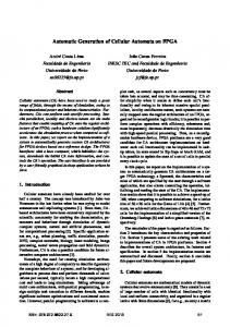
versal within a single plane of the 3D space, since it is just the 2D square-lattice SSM discussed above. To allow signals to get out of a single plane, mirrors can be applied to diagonal particles to deflect them onto cube-face diagonals outside of their original plane. A slightly simpler 3D scheme is shown in Figure 4b. Here we only use body and face diagonals, and body diagonals only collide when they are coplanar with a face diagonal. Since each face diagonal can only come from one pair of body diagonals, no collision-plane information is carried by face-diagonal particles. For mirrors, we can restrict ourselves to reflecting each body diagonal into one of the three directions that it could have been deflected into by a collision with another body diagonal. This is an interesting restriction, because it means that we can potentially make a momentum-conserving version of this model without mirrors, using only signals to deflect signals. Finally, the scheme shown in Figure 4c uses only face diagonals, with the heavier particle traveling half as fast as the particles that collide to produce it. As in Figure 4a, the slower particle carries a bit of collision-plane information. To accommodate the slower particles, the lattice needs to be twice as fine as in Figures 4a and 4b, but we’ve only shown one intermediate lattice site for clarity. Noting that three coplanar face-diagonals of a cube form an equilateral triangle, we see that this model, for particles restricted to a single plane, is exactly equivalent to the
Other Soft Sphere Models
In Figure 3b, we show a mass- and momentumconserving SSM collision on a triangular lattice, which corresponds to a reversible lattice gas model of computation in exactly the same manner as discussed above. Similarly, we can construct SSM’s in 3D. In Figure 4a, we see a mass and momentum conserving SSM collision using the face-diagonals of the cubes that make up our 3D grid. The resulting particle (gray) carries one bit of information about which of two possible planes the face-diagonals that created it resided in. In a corresponding diagram showing colliding spheres (a 3D version of Figure 2a), we would see that this information is carried by the plane along which the spheres are compressed. This model is uni6
(a)
(b)
(c)
Figure 4: 3D Soft Sphere Models. (a) Collisions using cube edges and cube-face diagonals. Each edge particle carries one bit of information about which of two planes the diagonal particles that created it were in. (b) Collisions using face and body diagonals. Two body-diagonal particles collide only if they are both coplanar with a face-diagonal. The resulting face-diagonal particle doesn’t carry any extra planar information, since there is a unique pair of body-diagonal particles that could have produced it. (c) Collisions using only face diagonals, with two speeds. If particles are confined to a single plane, this is equivalent to the triangular lattice model of Figure 3b. Again the slower particle must carry an extra bit of collision-plane information. triangular-lattice model pictured in Figure 3b. As in the model pictured in Figure 4b, the deflection directions that can be obtained from particle-particle collisions are sufficient for 3D routing, and so this model is also a candidate for mirrorless momentumconserving computation in three dimensions.
in [24], where it was shown that some 2D LGA’s of physical interest can compute any logical function. This paper did not, however, address the issue of whether such LGA’s can be spatially efficient models of computation, reusing spatial resources as ordinary computers do. There is also a new question about the generation of entropy (undesired information) which arises in the context of reversible momentum conserving computation models, and 5 Momentum conserving which we will address. With mirrors, any reversible models function can be computed in the SSM (or BBM) without leaving any intermediate results in the A rather unphysical property of the BBM, as well as computer’s memory[11]. Is this still true without of the related soft sphere models we have constructed, mirrors, where even the routing of signals requires an is the use of immovable mirrors. If the mirrors moved interaction with other signals? We will demonstrate even a little bit, they would spoil the digital nature of mirrorless momentum-conserving SSM’s that are these models. To be perfectly immovable, as we dejust as efficient spatially as an SSM with mirrors, mand, these mirrors must be infinitely massive, which and that don’t need to generate any more entropy is not very realistic. In this section, we will discuss than an SSM with mirrors. In the process we will SSM gases which compute without using mirrors, and illustrate some of the general physical issues involved hence are perfectly momentum conserving. in efficiently routing signals without mirrors. The issue of computation universality in momentum-conserving lattice gases was discussed 7
A
A
A
A
A
A
A
A
A A
A
A
1
A
1
(a)
1
(b)
Figure 5: Using streams of balls as mirrors. (a) A stream of 1’s (balls) diverts a signal A, but also makes two copies of the signal. (b) If dual-rail (complementary) signalling is used, signals can be cleanly reflected.
5.1
Reflections without mirrors
delaying one signal stream relative to the other, this technique requires the use of mirrors to insert comWe begin our discussion by replacing a fixed mirror pensating delays that resynchronize streams. If we’re with a constant stream of particles (ones), aimed at using streams of balls to act as mirrors, we have a the position where we want a signal reflected. This problem when these mirror streams have to cross sigis illustrated in Figure 5a. Here we show the 2D nals, or even each other. square-lattice SSM of Figure 2a, with a signal A beWe can deal with this problem by extending the ing deflected by the constant stream. Along with the non-interacting portion of our dynamics. In order to desired reflection of A, we also produce two undemake our SSM’s unconditionally digital, we already sired copies of A (one of them complemented). This require that balls pass through each other when too suggests that perhaps every bend in every signal path many try to pile up in one place. Thus it seems natwill continuously generate undesired information that ural to also use the presence of extra balls to force will have to be removed from the computer. signals to cross. The simplest way to do this is to add Figure 5b shows a more promising deflection. The a rest particle to the model—a particle that doesn’t only thing that has changed is that we have brought move. At a site “marked” by a rest particle, signals ¯ in A along with A, and so we now get a 1 coming will simply pass through each other. This is mass out the bottom regardless of what the value of A and momentum conserving, and is perfectly compatwas. Thus signals that are represented in compleible with continuous classical mechanics. Notice that mentary form (so-called “dual-rail” signals) can be we don’t actually have to change our SSM collision deflected cleanly. This makes sense, since each signal now carries one unit of momentum regardless of its rule to include this extra non-interacting case, since value, and so the change of momentum in the deflect- we gave the rule in the form, “these cases interact, ing mirror stream can now also be independent of the and in all other cases particles go straight.” Figure 6a shows an example of two signal paths crossing over a signal value. rest particle (indicated by a circle). Figure 6b shows an example of a signal crossover that doesn’t require a rest particle in the lattice gas An important use of mirrors in the BBM and in version of the SSM. Since LGA particles only interact SSM’s is to allow signals to cross each other with- at lattice sites, which are the corners of the grid, two out interacting. While signals can also be made to signals that cross as in this Figure cannot interact. cross by leaving regular gaps in signal streams and Such a crossover occurs in Figure 5b, for example.
5.2
Signal crossover
8
A
A
B
B
A
B
A B
(a)
(b)
Figure 6: Signals that cross. (a) The circle indicates a rest particle. Two signals cross at a rest particle without interacting. (b) Signals can also cross between lattice sites, where no interaction is possible. is only proportional to the surface area. We have the same kind of problem if we try to bring free energy (i.e., energy without information) into a volume. Using dual-rail signalling, we’ve seen that we have neat collisions available that don’t corrupt the deflecting mirror streams. We do not, however, avoid the surface to volume problem unless these clean mirror-streams can be reused: otherwise each reflec5.3 Spatially-efficient computation tion involves bringing in a mirror stream all the way from outside of the circuit, using it once, and then With the addition of rest particles to indicate signal sending the reflected mirror stream all the way out crossover, we can use the messy deflection of Figof the circuit. Thus if we can’t reuse mirror streams, ure 5a to build reusable circuitry and so perform the maximum number of circuit elements we can put spatially-efficient computation. The paths of the ininto a volume of space grows like the surface area coming “mirror streams” can cross whatever signals rather than like the volume! We will show that (at are in their way to get to the point where they are least in 2D) mirror streams can be reused, and conseneeded, and then the extra undesired “garbage” outquently momentum conservation doesn’t impair the put streams can be led away by allowing them to spatial efficiency of computations. cross any signals that are in their way. Since every mirror stream (which brings in energy but no information) and every garbage stream (which carries 5.4 Signal Routing away both energy and entropy) crosses a surface that encloses the circuit, the number of such streams that Even though we can reflect dual-rail signals and make we can have is limited by the area of the enclosing them cross, we still have a problem with routing sigsurface. Meanwhile, the number of circuit elements nals (actually two problems, but we’ll discuss the sec(and hence also the demand for mirror and garbage ond problem when we confront it). Figure 7a illusstreams) grows as the volume of the circuit[11, 4, 9]. trates a problem that stems from not being able to This is the familiar surface to volume ratio problem reflect signals at half-integer locations. Every reflecthat limits heat removal in ordinary heat-generating tion leaves the top A signal on the dark checkerboard physical systems: the rate of heat generation is pro- we’ve drawn—it can’t connect to an input on the light portional to the volume, but the rate of heat removal checkerboard. We can fix this by rescaling the circuit, Without the LGA lattice to indicate that no interaction can take place at this site, this crossover would also require a rest particle. To keep the LGA and the continuous versions of the model equivalent, we will consider a rest particle to be present implicitly wherever signals cross between lattice sites.
9
A
A
A
A A
A
A
A
A
A
A
A
A A
A
1
1
(a)
1
1
(b)
1
1
(c)
Figure 7: A signal routing constraint. (a) When signal pairs are deflected by a stream of 1’s, each component of the pair remains on the same checkerboard region of the space. (b) If we spread the signals so that pairs are twice as far apart, we can also rescale the mirror collision. (c) After rescaling, we can move the “mirror” to what would have originally been a half-integer position, and so avoid this constraint. spreading all signals twice as far apart (Figure 7b). Now the implicit crossover in the middle of Figure 7a must be made explicit. Notice also that the horizontal particle must be stretched—it too goes straight in the presence of a rest particle. Now we can move the reflection to a position that was formerly a halfinteger location (Figure 7c), and the A signal is deflected onto the white checkerboard.
5.5
¯ there is no reflection and they go straight. The A signal reflects off the constant-one input as in Fig¯ outputs. Notice ure 5a, to regenerate the A and A that if a rest particle were added in Figure 8a at the intersection of the A and B signals, the switch would ¯ would always go be stuck in the off position: B and B ¯ would get reflected straight through, and A and A by the constant-one, and come out in their normal position.
Dual-rail logic
We’ve seen that dual-rail signals can be cleanly routed. In order to use such signals for computation, we need to be able to build logic with dual-rail inputs and outputs. We will now see that if we let two dual-rail signals collide, we can form a switchgate[11], as shown in Figure 8a. The switch gate is a universal logic element that leaves the control input A unchanged, and routes the controlled input B to one of two places, depending on the value of A. Since each dual rail signal contains a 1, and since all collisions conserve the number of 1’s, all dual-rail logic gates need an equal number of inputs and outputs. Thus our three output switch-gate needs an extra input which is a dual-rail constant of 0. The switch gate (Figure 8a) is based on a reflection of the type shown in Figure 5b. If A=1 (Figure 8b), ¯ pair are reflected downward; if A=0 the B and B
5.6
A Fredkin Gate
In order to see that momentum conservation doesn’t impair the spatial efficiency of SSM computation, we first illustrate the issues involved by showing how mirror streams can be reused in an array of Fredkin gates[11]. A Fredkin gate has three inputs and three outputs. The A input, called the control, appears unchanged as the A output. The other two inputs either appear unchanged at corresponding outputs (if A=1), or appear interchanged at the corresponding outputs (if A=0). We construct a Fredkin gate out of four switch gates, as shown in Figure 9a. The first two switch gates are used forward, the last two switch gates are used backward (i.e., flipped about a vertical axis). The control input A is colored in solid gray, and we see it wend its way through the four switch
10
A
AB A+B
A
A
1
A
0
0
1
1
0
0
1
B
B
B
B
B
B
0 1
AB
0
A+B
1
(a)
B
0
B
1
B
B
0 1
0 1
(b)
(c)
Figure 8: A switch gate using dual-rail signalling. (a) The general case. The A signal either deflects B and ¯ or not, doing most of the work. We’ve highlighted the constant stream of ones by using dotted lines. B ¯ are reflected down, and the one is reflected the opposite way. (c) The case (b) The case A=1. B and B ¯ and they go straight. A=0. There is no interaction with B or B,
1
1
11
11
1
1 1
1
F
A
A
A
A
B
BA+CA
B
BA+CA
1
1
C
CA+BA
C
CA+BA
F
F
F
F
F
F
F
1
1 1
1
1
1
(a)
(b)
Figure 9: (a) A Fredkin gate. We construct a Fredkin gate out of four switch gates, two used forward, and two backward. Constant 1’s are drawn in lightly using dotted arrows. The path of the control signal A is shown in solid gray. If we added constant streams of 1’s along the four paths drawn as dotted lines without arrows, then the constant streams would be symmetrical about diagonal axes. (b) Because of the diagonal symmetry of this Fredkin gate construction, we can make an array of them, as indicated here, and reuse the constant streams of 1’s that act as signal mirrors. The upside down Fredkin gates are also Fredkin gates, but with the sense of the control inverted.
11
gates. Constant 1’s are shown using dotted gray arrows. In the case A=0, all four switch gates pass their controlled signals straight through, and so B and C interchange positions in the output. In the case A=1, all four switch gates deflect their controlled signals, and so B and C come out in the same positions they went in. Now notice the bilateral symmetry of the Fredkin gate implementation. We can make use of this symmetry in constructing an array of Fredkin gates that reuse the constant 1 signals. If we add an extra stream of constant 1’s along the four paths drawn as arrowless dotted lines (making these lie on the lattice involves rescaling the circuit), then the set of constant streams coming in or leaving along each of the four diagonal directions is symmetric about some axis. This means that we can make a regular array of Fredkin gates and upside-down Fredkin gates, as is indicated in Figure 9b, with the constants all lining up. These constants are passed back and forth between adjacent Fredkin gates, and so don’t have to be supplied from outside of the array. Since an upsidedown Fredkin gate is still a Fredkin gate, but with the sense of the control inverted, we have shown that constant streams of ones can be reused in a regular array of logic. We still have not routed the inputs and outputs to the Fredkin gates, and so we have another set of associated mirror-streams that need to be reused. The obvious approach is to create a regular pattern of interconnection, thus allowing us to again solve the problem globally by solving it locally. But a regular pattern of interconnected logic elements that can implement universal computation is just a universal CA: we should simply implement a universal CA that doesn’t have momentum conservation!
5.7
Implementing the BBMCA
The BBMCA is a simple reversible CA based on the BBM, with fixed mirrors[15, 17, 19]. It can be implemented as a regular array of identical logic blocks, each of which takes four bits of input, and produces four bits of output (Figure 10a). Each logic block exchanges one bit of data with each of the four blocks that are diagonally adjacent. The four bits of input
can be thought of as a pattern of data in a 2×2 region of the lattice, and the four outputs are the next state for this region. According to the BBMCA rule, certain patterns are turned into each other, while other patterns are left unchanged. This rule can be implemented by a small number of switch gates, as is indicated schematically in Figure 10b. We first implement a demultiplexer F , which produces a value of 1 at a given output if and only if a corresponding 2×2 pattern appears in the inputs. Patterns that don’t change under the BBMCA dynamics only produce 1’s in the outputs labeled “other.” The demultiplexer is a combinational circuit (i.e., one without feedback). The inverse circuit F −1 is simply the mirror image of F , obtained by reflecting F about a vertical axis. In between F and F −1 we wire together the cases that need to interchange. This gives us a bilaterally symmetric circuit which implements the BBMCA logic block in the same manner that our circuit of Figure 9a implemented the Fredkin gate. Note that the overall circuit is its own inverse, as any bilaterally symmetric combinational SSM circuit must be. Now we would like to connect these logic blocks in a uniform array. We will first consider the issue of sharing the mirror streams associated with the individual logic blocks, and then the issue of sharing the mirror streams associated with interconnecting the four inputs and outputs. In Figure 11a we see a schematic representation of our BBMCA block. It is a combinational circuit, with signals flowing from left to right. The number of signal streams flowing in along one diagonal direction is equal to the number flowing out along the same direction—this is true overall because it’s true of every collision! In particular, since the four inputs and outputs are already matched in the diagram, the mirror streams must also be matched— there are an equal number of streams of constant 1’s coming in and out along each direction. The input streams will not, however, in general be aligned with the output streams. If we can align these, then we can make a regular array of these blocks, with mirrorstream outputs of one connected to the mirror-stream inputs of the next. In Figure 11b we show how to align streams of ones. Due to the bilateral symmetry of the BBMCA circuit, every incoming stream that we would like to
12
AB DC
10 00
AB DC
0 0 0 0 0 1 1 0 0 1
A
AB DC
B
AB DC
F
C
AB DC
D
AB DC
0 1 1 0 0 0 0 1
0 0 0 1
0 0 0 1
1 0 0 0
A'
F
-1
10 01
1 0
B' C' D'
01 10
other
(a)
1 0 0 0
other
(b)
Figure 10: Emulating the BBMCA using an SSM. (a) The BBMCA can be implemented as a 2D array of identical blocks of logic, each of which processes four bits at a time. The bits that are grouped together in one step go to four different diagonally adjacent blocks in the next step. (b) We construct a circuit out of switch gates to implement the BBMCA logic block. The first half of the circuit (F ) produces a set of outputs that are each one only if the four BBMCA bits have some particular pattern. The second half (F −1 ) is the mirror image of the first. In between, the cases that interchange are wired to each other.
B
A A B F C D
1 0 0 0 0 0 0 1 1 0 0 1
0 0 0 1 1 0 0 0 0 1 1 0
1 0 0 0 0 0 0 1
0 0 0 1 1 0 0 0
10 01 01 10
A' B' F
A'
B' A B
-1
C
C' D'
D
A
(a)
B
(b)
C
D
(c)
Figure 11: Symmetrizing signal paths so that adjacent BBMCA logic blocks can share their mirror constants. (a) The BBMCA block circuit is bilaterally symmetric, with an equal number of constants flowing in or out along each of the four diagonal directions. (b) Symmetric pairs of constant 1’s can be shifted vertically in order to align the “mirror streams” so that the blocks can be arrayed. (c) The wiring of the four BBMCA signal inputs (and outputs) to each block is also bilaterally symmetric, so the same alignment techniques should apply.
13
shift up or down on one side is matched by an outgoing stream that needs to be shifted identically on the other side. Thus we will shift streams in pairs. To understand the diagram, suppose that A and B are constant streams of ones, with B going into a circuit below the diagram, and A coming out of it. Now suppose that we would like to raise A and B to the positions labeled A0 and B0 . If a constant stream of horizontal particles is provided midway in between the two vertical positions, then we can accomplish this as shown. The constant horizontal stream splits at the first position without a rest particle. It provides the shifted A0 signal, and a matching stream of ones collides with the original A signal. The resulting horizontal stream is routed straight across until it reaches B, where an incoming stream of ones is needed. Here it splits, with the extra stream of ones colliding with the incoming B0 signal to restore the original horizontal stream of ones, which can be reused in the next block of the array of circuit blocks to perform the same function. The net effect is that the mirror streams A and B coming out of and into a circuit have been replaced with new streams that are shifted vertically. By reserving some fraction of the horizontal channels for horizontal constants that stream across the whole array, and reserving some channels for horizontal constants that connect pairs of streams being raised, we can adjust the positions of the mirror streams as needed. Note that a mirror pair can be raised by several smaller shifts rather than just one large shift, in case there are conflicts in the use of horizontal constants. Exactly the same arrangement can be used to lower A0 and B0 going into and out of a circuit above the diagram. If we flip the diagram over, we see how to handle pairs of streams going in the opposite directions.
5.8
Signal routing revisited
So far, we have only constructed circuits without feedback—all signal flow has been left to right. Because of the 90◦ rotational symmetry of the SSM, we might expect that feedback isn’t a problem. When we decided to use dual-rail signalling, however, we broke this symmetry. The timing of the dual rail signal pairs is aligned vertically and not horizontally. In Figure 12a, we see the problem that we encounter when we try to reflect a right-moving signal back to the left. A signal that passed the input position labeled A at an even time-step collides with an un¯ at an odd timerelated signal that passed input A step. These two signals need to be complements of each other in order to reconstitute the reflecting mirror stream. Thus we only know how to reflect signals vertically, not horizontally! We will discuss two ways of fixing this problem. Both involve using additional collisions in the SSM. The first method we describe is more complicated, since it adds additional particles and velocities to the model, but is more obvious. The idea is that we can resynchronize dual-rail pairs by delaying one signal. We do this by introducing an interacting rest particle (distinct from our previously introduced noninteracting rest particle) with the same mass as our diagonally-moving particles. The picture we have in mind is that if there is an interacting rest particle in the path of a diagonally-moving particle, then we can have a collision in which the moving particle ends up stationary, and the stationary particle ends up moving. During the finite interval while the particles are colliding, the mass is doubled and so (from momentum conservation) the velocity is halved. By picking the head-on impact interval appropriately, the new stationary particle can be deposited on a lattice site, so that the model remains digital. This is illustrated in Figure 12b. Here the square block inNow we note that the wiring of the four signal in- dicates the interacting rest particle. This is picked puts and outputs in our BBMCA array also has bilat- up in a collision with a diagonal-moving particle to eral symmetry, about a horizontal axis (Figure 11c). produce a half-speed double-mass particle indicated Thus it seems that we should be able to apply the by the short arrow. Note that adding this delay colsame technique to align the mirror streams associ- lision requires us to make our lattice twice as fine to ated with this routing, in order to complete our con- accommodate the slower diagonal particles. It adds struction. But there is a problem. five new particle-states to our model (four directions 14
A
A
1
A
A
1
A A
A
??
1
A A
(a)
(b)
(c)
Figure 12: Reflecting signals back. (a) Dual rail pairs that are synchronized by column only reflect correctly off “horizontal mirrors.” If we try to bounce them off a “vertical mirror,” signals from different times interact. (b) This can be fixed by providing a way to slow down a signal. The rule for adding slower particles involves refining the lattice to admit a half-speed double-mass diagonal particle, and adding a single-mass rest particle (square block in the diagram). When a soft sphere collides with an equally massive sphere at rest, the first slows down as the second speeds up (giving a net speed of 1/2), and then the sphere that was at rest proceeds. (c) Using our “no-interaction” rest particle to extend the lifetime of the half-speed diagonal particle, we can change a column-synchronized pair into a row-synchronized pair, and then back. for the slow particle, and an interacting rest particle). The model remains, however, physically “realistic” and momentum conserving. Figure 12c illustrates the use of this delay to reflect a rightgoing signal leftwards. We insert a delay in the ¯ path both before the mirror-stream collision and A afterward, in order to turn the plane of synchronization 180◦ , turning it 90◦ at a time. Notice that we use a non-interacting rest particle (round) to extend the lifetime of the half-speed diagonal particle. In addition to complicating the model, this delay technique adds an extra complication to showing that momentum conservation doesn’t impair spatial efficiency. Signals are delayed by picking up and later depositing a rest particle. In order to reuse circuitry, we must include a mechanism for putting the rest particle back where it started before the next signal comes through. Since we can pick this particle up from any direction, this should be possible by using a succession of constant streams coming from various directions, but these streams must also be reused. We won’t try to show that this can be done here—we will pursue an easier course in the next Section. It would be simpler if the moving particle was de-
posited at the same position that the particle it hit came from, so that no cleanup was needed. Unfortunately, this necessarily results in no delay. Since the velocity of the center of mass of the two particles is constant, if we end up with a stationary particle where we started, the other particle must exactly take the place of the one that stopped.
5.9
A simpler extension
We can complete our construction without adding any extra particles or velocities to the model. Instead, we simply add some cases to the SSM in which our normal soft-sphere collisions happen even when there are extra particles nearby. The cases we will need are shown in Figure 13. In this diagram, we show each forward collision in one particular orientation—collisions in other orientations and the corresponding inverse collisions also apply. The first case is the SSM collision with nothing else around. The second case is a forward and backward collision simultaneously—this will let us bounce signals back the way they came. The third case has at least two spectators, and possibly a third (indicated
15
(a)
(b)
(c)
Figure 13: A 2D square-lattice SSM. Particles go straight unless they interact. One sample orientation is shown for each interacting case. The inverse cases also apply. (a) Basic collision. (b) Same collision and its inverse operating in two opposite directions simultaneously. (c) Same collision as (a), but with “spectator particles” present. The dotted-arrow particle may or may not be present, and may come from below instead (i.e., flipped orientation). Spectators go straight. by a dotted arrow). The collision proceeds normally, and all spectators pass straight through. This case will allow us to separate forward and backward moving signals. As usual, all other cases go straight. In particular, we will depend for the first time on headon colliding particles going straight. We have not used any head-on collisions in our circuits thus far, and so we are free to define their behavior here.
these backward-going signals, and so they go straight through. The vertical constants were needed to break the symmetry, so that it’s unambiguous which signals should interact. This separation uses the extra spectator-particle cases added to our rule in Figure 13c. As we will discuss, in a triangular-lattice SSM the separation at mirrors doesn’t require any vertical constants at the mirrors (see Section 5.10).
Figure 14a shows how two complementary sets of dual-rail signals can be reflected back the way they came. We show the signals up to the moment where they come to a point where they collide with the two constant streams. In the case where A=1, we have four diagonal signals colliding at a point, and so everything goes straight through. In particular, the constant streams have particles going in both directions (passing through each other), and the signal particles go back up the A paths without interacting with oncoming signals. In the case where A=0, we use our new “both-directions” collision, which again sends all particles back the way they came. Thus we have succeeded in reversing the direction of a signal stream.
Finally, Figure 15 shows how we can arrange to always have two complementary dual-rail pairs collide whenever we need to send a signal backward. Figure 15a shows an SSM circuit with some number of dual-rail pairs. In each pair, the signals are synchronized vertically, with the uncomplemented signal on top. Figure 15b shows the same gate flipped vertically. The collisions that implement the circuit work perfectly well upside-down, but both the inputs and the outputs are complemented by this inversion. For example, in Figure 15c, we have turned a switch-gate upside down. If we relabel inputs and outputs in conventional order, then we see that this gate performs a logical OR where the original gate performed an AND. In Figure 15d, we take our BBMCA logic block Figure 14b shows a mirror with all signals moving of Figure 10b and add a vertically reflected copy. This from left to right. We’ve added in vertical constant- pair of circuits, taken together, has both vertical and streams in two places, which don’t affect the opera- horizontal symmetry. Given quad-rail inputs (dual tion of the “mirror.” These paths have a continual rail inputs along with their dual-rail complements), stream of particles in both the up and down direc- it produces corresponding quad-rail outputs, which tions, and so these particles all go straight (head-on can be reflected backward using the collision of Figcollisions). In Figure 14c, we’ve just shown signals ure 14a, and separated at mirrors, as shown in Figcoming into this mirror backward (with the forward ure 14c. Now note that the constant-lifting technique paths drawn in lightly). This mirror doesn’t reflect of Figure 11b works equally well even if all of the con16
A
1
A
1
A
1
1
1
A
A
1
A
(a)
1
1
1
A
A
A
A
B
1
B
1
1
B
1
(b)
1
B
(c)
Figure 14: A way to reflect signals back, without refining the lattice or adding extra particles. (a) If we have two dual rail signal-pairs (one the complement of the other), then they can be bounced straight backward along the same paths they came in on by bringing all the signals to one point at which two mirror signals impinge. In either case (A=0 and A=1), the constant 1’s that reflect these signals are also reversed along their paths. (b) The thick vertical dotted line-segments indicate constants of one that are moving in both directions at the indicated locations. This is otherwise a normal reflection of a signal—the extra vertical streams don’t interfere with the operation of the “mirror.” (c) If a backward propagating signal comes ¯ then it is not reflected by this forward mirror—such a mirror separates the in from the right (B and B), backward moving stream from the forward stream.
A
A'
C
A'
C
B'
B
B'
B
C
C'
A
C
C'
A
A B B
logic circuit
C'
flipped logic circuit
C'
1
A+B
0
AB
B
B' B
B' A'
A
A
A'
A
A AB A+B
(a)
(b)
(c)
A A B B C C D D D D C C B B
A' A'
F
F
-1
F
F
-1
A A
B' B' C' C' D' D' D' D' C' C' B' B' A' A'
(d)
Figure 15: DeMorgan inversion. (a) A logic circuit with dual-rail inputs. In each input pair, the complemented signal lies below the uncomplemented one. (b) If this circuit is flipped vertically, the operation of the circuit is unchanged, but it operates upon inputs that are complemented (according to our conventions) and produces outputs that are also complemented. (c) The switch gate of Figure 8a, flipped vertically. Inputs and outputs have been relabeled to call the top signal in each dual-rail pair “uncomplemented.” (d) The BBMCA logic circuit of Figure 10b has been mirrored vertically to produce a vertically symmetric circuit which has complementary pairs of dual-rail pairs.
17
AB
1
A
1
A+B
A
A
A A
B
(a)
A
1
A
1
B
A
A
A
A
(b)
0
AB
1
A+B
(c)
A
(d)
Figure 16: An SSM gas on the triangular lattice which allows signal feedback. (a) Two speed-2 particles collide and turn into a speed-1 particle with twice the mass. This decays back into two speed-2 particles. If an extra “spectator” speed-2 particle comes in as shown with a dotted-arrow (or the flip of these cases), it passes straight through. Collisions can happen both forward and backward simultaneously. In all other cases, particles go straight. (b) Constants act as mirrors for dual-rail signals. (c) This is a switch gate. Other combinational circuits from the square-lattice SSM can be similarly stretched vertically to fit onto the triangular lattice. (d) The third collision case in the rule makes signals bounce back the way they came. Backward-going signals will separate at a mirror such as is shown in (b). stant streams have 1’s flowing in both directions simultaneously, by virtue of the bidirectional collision case of Figure 13b. Thus we are able to apply the constant-symmetrizing technique to mirror streams that connect the four signals between our BBMCA logic blocks (Figure 11c), and complete our construction.
nals are sent back the way they came, is shown in Figure 16d. This of course also means that the corresponding 3D model (Figure 4c) can perform efficient momentum-conserving computation, at least in a single plane. If we have a dual-rail pair in one plane of this lattice, and its dual-rail complement directly below it in a parallel plane, this combination can be deflected cleanly in either of two planes by a pair 5.10 Other lattices of constant mirror-streams. Thus it seems plausible All of this works equally well for an SSM on the tri- that this kind of discussion may be generalized to angular lattice, and is even slightly simpler, since we three dimensions, but we won’t pursue that here. don’t need to add extra constant streams at mirrors where forward and backward moving signals separate (as we did in Figure 14c). The complete rule is given 6 Relativistic CA’s in Figure 16a: the dotted arrow indicates a position where an extra “spectator” particle may or may not We have presented examples of reversible lattice gases come in. If present, it passes straight through and that support universal computation and that can doesn’t interfere with the collision. In Figures 16b be interpreted as a discrete-time sampling of the and 16c, we see how mirrors and switch-gates (and classical-mechanical dynamics of compressible balls. similarly any other square-lattice SSM combinational We would like to present here an alternative interprecircuit) can simply be stretched vertically to fit onto tation of the same models as a discrete-time sampling the triangular lattice. A back-reflection, where sig- of relativistic classical mechanics, in which kinetic en18
ergy is converted by collisions into rest mass and then back into kinetic energy. For a relativistic collision of some set of particles, both relativistic energy and relativistic momentum are conserved, and so: X X X X Ei = Ei0 , Ei~vi = Ei0~vi0 , i
i
i
i
where the unprimed quantities are the values for each particle before the collision, and the primed quantities are after the collision. These equations are true regardless of whether the various particles involved in the collision are massive or massless. Now we note that for any mass and momentum conserving lattice gas, X X X X mi = m0i , mi~vi = m0i~vi0 , i
i
i
i
and so we need only reinterpret what is normally called “mass” in these models as relativistic energy in order to interpret the collisions in such a lattice gas as being relativistic. If all collisions are relativistically conservative, then the overall dynamics exactly conserves relativistic energy and momentum, regardless of the frame of reference in which the system is analyzed. Normal non-relativistic systems have separate conservations of mass and non-relativistic energy— a property that the collisions in most momentumconserving lattice gases lack. Thus we might argue that the relativistic interpretation is more natural in general. In the collision of Figure 2b, for example, we might call the incoming pair of particles “photons,” each with unit energy and unit speed. The two photons collide, and the vertical components of their √ momenta cancel, producing a√slower moving (v = 1/ 2) massive particle (m = 2) with energy 2 and with the same horizontal component of momentum as the original pair. After one step, the massive particle decays back into two photons. At each step, relativistic energy and momentum are conserved. As is discussed elsewhere[18, 19], macroscopic relativistic invariance could be a key ingredient in constructing CA models with more of the macroscopic richness that Nature has. If a CA had macroscopic
relativistic invariance, then every complex macroscopic structure (assuming there were any!) could be set in motion, since the macroscopic dynamical laws would be independent of the state of motion. Thus complex macroscopic structures could move around and interact and recombine. Any system with macroscopic relativistic symmetry is guaranteed to also have the relativistic conservations of energy and momentum that go along with it. As Fredkin has pointed out, a natural approach to achieving macroscopic symmetries in CA’s is to start by putting the associated microscopic conservations directly into the CA rule—we certainly can’t put the continuous symmetries there! Momentum and mass conserving LGA models effectively do this. Of course, merely reinterpreting the microscopic dynamics of lattice gases relativistically doesn’t make their macroscopic dynamics any richer. One additional microscopic property that we can look for is the ability to perform computation, using space as efficiently as is possible: this enables a system to support the highest possible level of complexity in a finite region. Microscopically, SSM gases have both a relativistic interpretation and spatial efficiency for computation. What we would really like is a dynamics in which both of these properties persist at the macroscopic scale. If we are trying to achieve macroscopic relativistic invariance along with efficient macroscopic computational capability, we can see that one potential problem in our “bounce-back” SSM gases (Figures 13 and 16) is a defect in their discrete rotational symmetry. Dual-rail pairs of signals aligned in one orientation can’t easily interact with dual-rail pairs that are aligned in a 60◦ (triangular lattice) or 90◦ (square lattice) rotated orientation. If this causes a problem macroscopically, we can always try adding individual signal delays to the model, as in Figure 12b. This may have macroscopic problems as well, however, since turning signals with the correct timing requires several correlated interactions. Of course the reason we adopted dual-rail signalling to begin with was to avoid mixing logic-value information with signal momentum—every dual-rail signal has unit momentum and can be reflected without “measuring” the logic value. Perhaps we should simply decou-
19
0
0
!"
!"
!=1
(a)
!=0
!"
!=1
!"
"=1
!"
"=1
!"
0
!"
0
!"
(b)
(c)
!
(d)
Figure 17: A computation-universal LGA in which ones and zeros have the same momentum. (a) We use three kinds of particles that interact. The three cases shown, plus rotations, inversions and the time-reversal of these cases, are all of the interactions. In all other cases, particles don’t interact. (b) We use the solidblack particles to represent “ones” and the dotted particles to represent “zeros”. If only a single one comes into a “collision,” none of the interaction cases applies, and so everything goes straight. (c) If two ones collide, they turn into a third kind of particle (shown as a wavy arrow), which is deflected by a zero (and deflects the zero). The inverse interaction recreates the two ones, displaced inwards from their original paths (as in an SSM collision). (d) The wavy particle also deflects (and is deflected by) a one. ple these two quantities at the level of the individual particle, and use some other degree of freedom (other than presence or absence of a particle) to encode the logic state (eg., angular momentum). An example of a model which decouples logic values and momentum is given in Figure 17. In Figure 17a, we define a rule which involves three kinds of interacting particles. Figures 17b and 17c show how an SSM style collision-gate can be realized, using one kind of particle to represent an intermediate state. Single ones go straight, whereas pairs of ones are displaced inwards. Both ones and zeros are deflected by the wavy “mirror” particles, which can play the role of the mirror-streams in our earlier constructions. Deflecting a binary signal conserves momentum without recourse to dual rail logic, and without contaminating the mirror-stream. Adding rest particles to this model allows signals to cross (since the rule is, “in all other cases particles don’t interact”). Models similar to this “proto-SSM” would be interesting to investigate on other lattices, in both 2D and 3D. The use of rest particles to allow signals to cross in this and earlier rules raises another issue connected
with the macroscopic limit. If we want to support complicated macroscopic moving structures that contain rest particles, we have to have the rest particles move along with them! (Or perhaps use moving signals to indicate crossings.) If we want to make rest particles “move,” they can’t be completely noninteracting. Thus we might want to extend the dynamics so that rest particles can both be created and destroyed. This could be done by redefining some of the non-interacting collision cases that have not been used in our constructions—we have actually used very few of these cases. These collisions would be different from the springy collision of Figure 2a. Even a single-particle colliding with a rest particle can move it (as in Figure 12b for example).
These are all issues that can be approached both theoretically, and by studying large-scale simulations[19].
20
7
Semi-classical models of dynamics
The term semi-classical has been applied to analyses in which a classical physics model can be used to reproduce properties of a physical system that are fundamentally quantum mechanical. Since the finite and extensive character of entropy (information) in a finite physical system is such a property[2], all CA models can in a sense be considered semi-classical. It is interesting to ask what other aspects of quantum dynamics can be captured in classical CA models. One such aspect is the relationship in quantum systems between energy and maximum rate of state change. A quantum system takes a finite amount of time to evolve from a given state to a different state (i.e., a state that is quantum mechanically orthogonal). There is a simple relationship between the energy of a quantum system in the classical limit and the maximum rate at which the system can pass through a succession of distinct (mutually orthogonal) quantum states. This rate depends only on how much energy the system has. Suppose that the quantum mechanical average energy E (which is the energy that appears in the classical equations of motion) is measured relative to the system’s groundstate energy, and in units where Planck’s constant h is one. Then the maximum number of distinct changes that can occur in the system per unit of time is simply 2E, and this bound is always achieved by some state[20]. Now suppose we have an energy-conserving LGA started in a state with total energy E, where E is much less than the maximum possible energy that we can fit onto the lattice. Suppose also that the smallest quantity of energy that moves around in the LGA dynamics is a particle with energy “one.” Then with the given energy E, the maximum number of spots that can possibly change on the lattice in one time-step is 2E (just as in the quantum case): E smallest energy particles can each leave one spot and move to another, each causing two changes if none of them lands on a spot that was just vacated by another particle. Since the minimum value of ∆E is 1 in this dynamics, and the minimum value of ∆t is
1 since this is our integer unit of time, it is consistent to think of this as a system in which the minimum value of ∆E∆t is 1 (which for a quantum system would mean h = 1). Thus simple LGA’s such as the SSM gases reproduce the quantum limit in terms of their maximum rate of dynamical change. This kind of property is interesting in a physical model of computation, since simple models that accurately reflect real physical limits allow us to ask rather sharp questions about quantifying the physical resources required by various algorithms (cf. [9]).
8
Conclusion
We have described soft sphere models of computation, a class of reversible and computation-universal lattice gases which correspond to a discrete-time sampling of continuous classical mechanical systems. We have described models in both 2D and 3D that use immovable mirrors, and provided a technique for making related models without immovable mirrors that are exactly momentum-conserving while preserving their universality and spatial efficiency. In the context of the 2D momentum-conserving models, we have shown that it is possible to avoid entropy generation associated with routing signals. For all of the momentum conserving models we have provided both a non-relativistic and a relativistic interpretation of the microscopic dynamics. The same relativistic interpretation applies generally to mass and momentum conserving lattice gases. We have also provided a semi-classical interpretation under which these models give the correct physical bound on maximum computation rate. It is easy to show that reversible LGA’s can all be turned into quantum dynamics which reproduce the LGA state at integer times[16]. Thus SSM gases can be interpreted not only as both relativistic and nonrelativistic systems, but also as both classical and as quantum systems. In all cases, the models are digital at integer times, and so provide a link between continuous physics and the dynamics of digital information in all of these domains, and perhaps also a bridge linking informational concepts between these domains.
21
Acknowledgements
[12] D. Griffeath and C. Moore (eds.), New Constructions in Cellular Automata, Oxford University Press (2003).
This work was supported by DARPA under contract number DABT63-95-C-0130. This work was stimulated by the SFI Constructive CA workshop.
[13] U. Frisch, B. Hasslacher and Y. Pomeau, “Latticegas automata for the navier-stokes equation,” Phys. Rev. Lett. 56, 1505–1508 (1986).
References
[14] J. Hardy, O. de Pazzis and Y. Pomeau, “Molecular dynamics of a classical lattice gas: transport properties and time correlation functions,” Phys. Rev. A 13, 1949–1960 (1976).
[1] A. Adamatzky (ed.), Collision Based Computation, Springer Verlag (2002). [2] R. Baierlein, Atoms and information theory: an introduction to Statistical Mechanics, San Francisco: W. H. Freeman (1971). [3] E. Banks, “Information Processing and Transmission in Cellular Automata,” Tech. Rep. MAC TR81, MIT Project MAC, Cambridge 1971. [4] C. H. Bennett, “The thermodynamics computation—a review,” in [10, p. 905–940].
[15] N. Margolus, “Physics-like models of computation,” in [7, p. 81–95]; reprinted in [25] and in [1]. [16] N. Margolus, “Quantum computation,” New Techniques and Ideas in Quantum Measurement Theory (D. Greenberger, ed.), New York Academy of Sciences, 487–497 (1986). [17] N. Margolus, Physics and computation, Ph.D. Thesis, Massachusetts Institute of Technology, Cambridge MA 1987.
of
[5] R. D’Souza, and N. Margolus, “Thermodynamically reversible generalization of diffusion limited aggregation,” Physics Review E 60:1, 264–274 (1999), arXiv:cond-mat/9810258. [6] R. D’Souza, Macroscopic order from reversible and stochastic lattice growth models, PhD. Thesis (Physics), Massachusetts Institute of Technology, Cambridge MA, August 1999. [7] D. Farmer, T. Toffoli and S. Wolfram (eds.), Cellular Automata, Amsterdam: North-Holland (1984); book reprinted from Physica D 10:1/2 (1984). [8] R. P. Feynman, Feynman Lectures on Computation, edited by J. G. Hey and R. W. Allen. Reading, MA: Addison-Wesley, 1996.
[18] N. Margolus, “A bridge of bits,” in [23, 253–257]. [19] N. Margolus, “Crystalline Computation,” in Feynman and Computation (Hey, ed.), Reading MA: Perseus Books, 267–305 (1998), arXiv:comp-gas/9811002. [20] N. Margolus and L. Levitin, “The maximum speed of dynamical evolution,” Physica D 120:1/2, 188– 195 (1998), arXiv:quant-ph/9710043. [21] N. Margolus, “An Embedded DRAM Architecture for Large-Scale Spatial-Lattice Computations,” in The 27th Annual International Symposium on Computer Architecture. IEEE, 149–160 (2000). [22] N. Margolus, “Universal CA’s based on the collisions of soft spheres,” in [1, 107–134] and [12, 231–260].
[9] M. P. Frank, Reversibility for efficient computing, Ph.D. Thesis, Massachusetts Institute of Technology AI Laboratory, Cambridge MA 1999. [10] E. Fredkin, R. Landauer and T. Toffoli (eds.), Proceedings of the Physics of Computation Conference, in Int. J. Theor. Phys., issues 21:3/4, 21:6/7, and 21:12 (1982). [11] E. Fredkin and T. Toffoli, “Conservative logic,” in [10, p. 219–253] and reproduced in [1].
22
[23] D. Matzke (ed.), Proceedings of the Workshop on Physics and Computation—PhysComp ’92, Los Alamitos, CA: IEEE Computer Society Press, 1993. [24] C. Moore and M. G. Nordahl, “Lattice Gas Prediction is P-complete,” Santa Fe Institute Working Paper 97-04-034, arXiv:comp-gas/9704001. [25] S. Wolfram, Theory and Applications of Cellular Automata, World Scientific (1986).