unknown sensor noise as well as channel bandwidth limitation. This paper ... Section 5 describes an extension of the universal DES to the noisy channel case,.
Universal Decentralized Estimation in a Bandwidth Constrained Sensor Network∗ Zhi-Quan Luo† June, 2003
Abstract Consider a situation where a set of distributed sensors and a fusion center wish to cooperate to estimate an unknown parameter over a bounded interval [−U, U ]. Each sensor collects one noise-corrupted sample, performs a local estimation, and transmits a message to the fusion center, while the latter combines the received messages to produce a final estimate. This paper investigates optimal local estimation and final fusion schemes under the constraint that the communication from each sensor to the fusion center must be an one-bit binary message. Such binary message constraint is well motivated by the bandwidth limitation of the communication links, and by the limited power budget of local sensors. In the absence of bandwidth constraint and assuming the noises are bounded to the interval [−U, U ], additive, independent but otherwise unknown, the classical estimation theory 2 suggests that a total of O( U² ) sensors are necessary and sufficient in order for the sensors and the fusion center to jointly estimate the unknown parameter within ² mean squared error. It is shown in this paper that the same remains true even with the binary message constraint. Furthermore, the optimal decentralized estimation scheme suggests allocating 1 1 2 of the sensors to estimate the first bit of the unknown parameter, 4 of the sensors to estimate the second bit, and so on.
∗
This research is supported in part by the Natural Sciences and Engineering Research Council of Canada, Grant No. OPG0090391 and by the Canada Research Chair Program. † Part of this research was performed while the author was with the Department of Electrical and Computer Engineering, McMaster University, Hamilton, Ontario L8S 4K1, Canada. His present address is Department of Electrical and Computer Engineering, University of Minnesota, 200 Union Street SE, Minneapolis, MN 55455.
1
Introduction
The current and future wireless sensor networks usually deploy a large number of inexpensive sensors whose dynamic range, resolution and power can be severely limited. Moreover, there can be physical limitations in the communication links from the sensors back to a central site (also known as fusion center). In such cases, local data quantization/compression is not only a necessity, but also an integral part of the design of sensor networks. In addition, the sensor observations are usually corrupted by noises whose distribution can be difficult to characterize in practice, especially for large networks. As a result, a main challenge in sensor network research is to design optimal decentralized detection/estimation schemes in the presence of unknown sensor noise as well as channel bandwidth limitation. This paper considers a situation where a set of distributed sensors and a fusion center wish to corporate to estimate a parameter in the presence of unknown sensor noises. Each sensor collects one noise-corrupted sample, performs a local estimation, and transmits a binary (0 or 1) message to the fusion center, while the latter combines the received bits to produce a final estimate. The binary message constraint is well motivated by the bandwidth limitation of the communication links, and by the limited power budget of local sensors. The goal of this paper is to study the impact of this bandwidth constraint on the optimal decentralized estimation schemes (DES for short) and on the number of sensors required to compute an ²-estimator of the unknown parameter. (Upon first examination, it is not clear whether such a DES even exists for each ² > 0, if the sensors are allowed to transmit only binary messages.) Throughout this paper, it is assumed that the sensors do not communicate with one another, and there is no feedback from the fusion center to the sensors. In the absence of bandwidth constraint and assuming the sensor noises are additive, independent but otherwise unknown, the classical estimation theory suggests that a total of O(1/²) sensors are necessary and sufficient in order for the sensor network to jointly estimate the unknown parameter within ² mean squared error. Somewhat surprisingly, it is shown in this paper that the same remains true even with the binary message constraint. In other words, the communication bandwidth constraint only results in a constant factor increase of the number of sensors required. Furthermore, the optimal DES derived in this paper has an intuitively appealing interpretation: 21 of the sensors should be assigned to estimate the first bit of the unknown parameter, 14 of the sensors to estimate the second bit, and so on. There has been a long history of research activities in decentralized detection/estimation under various network models. The most commonly used network model is the one where each sensor processes its respective measurement and transmits the result over a communication channel to a fusion center. For example, the problem of decentralized detection was analyzed in [16] under this network model and the assumption that the channels are reliable and the sensor observations are conditionally independent with known distributions. In the absence
1
of conditional independence assumption, the problem of determining the optimal strategy for decentralized detection was shown to be NP-hard [18]. Various extensions of these results, especially for large scale networks, are summarized in the survey paper [17]. The decentralized detection problem with communication constraint was studied in [12] whereby the sensors employ a “send/no send” strategy, effectively reducing the communication requirement from the sensors to the fusion center. In an earlier study [4], the same problem was considered under a more general information theoretic framework. In both of these studies [4, 12], the joint distribution of the sensor observations is assumed known and is used in the design of decentralized detection strategies. The problem of decentralized estimation has also been well-studied, first in the context of distributed control [1, 14] and tracking [19], later in data fusion [2, 5], and most recently in wireless sensor networks [8, 9]. Among these studies, the prevailing assumption has been that the joint distribution of the sensor observations is known, with some also making the additional assumption that the communication links can transmit real values and are distortionless. In the case where the communication links can only transmit discrete signals, the work of [3, 8, 9, 13] addressed various design and implementation issues using the knowledge of joint distribution of sensor data. Without the knowledge of noise distribution, the work of [6] proposed to use a training sequence to aid the design of local data quantization strategies. Our work differs from these studies in that it does not require the knowledge of noise distributions nor the use of a training sequence. In other words, the optimal DES derived in this paper is universal. Moreover, this scheme satisfies the binary message constraint and requires minimal (a constant factor of 4) increase in the number of sensors required. Our paper is organized as follows. In Section 2, we introduce the basic mathematical formulation of DES and the notion of universal estimator. Section 3 studies the optimal design of DES for the case where the noise probability density function is known, while assuming the sensor messages must be one binary bit. The case with unknown noise distribution is considered in Section 4 where an universal decentralized linear ²-estimator is presented. It is shown that this design is within a constant factor to the best possible in terms of the number of sensors required. Section 5 describes an extension of the universal DES to the noisy channel case, while Section 6 contains some computer simulation results illustrating the performance of the new universal DES and comparing it with the theoretical bounds. The final section (Section 7) contains some concluding remarks and suggestions for future research. Our notations are fairly standard. For any real number x ∈ R, we use dxe to signify the smallest integer upper bound of x (also known as the ceiling of x). For a real valued function g : R → R, we use Range(g) = {g(u) : u ∈ R} to denote the range of the mapping g, and use Supp(g) = {u : g(u) 6= 0} to denote the support of g (i.e., the region where g is non-vanishing).
2
2
Formulation and Preliminaries
Consider a set of K distributed sensors, each making observations on an unknown parameter θ ∈ [−V, V ], with V > 0 a given constant. The observations are corrupted by noise and are described by xk = θ + nk , k = 1, 2, ..., K, (2.1) where {ni : i = 1, 2, ..., K} are additive noise random variables. We assume the noise random variables are i.i.d., zero mean, and bounded to, say, [−U, U ] with a probability density function (or p.d.f. for short) p(u), where U > 0 is a given constant. Let µZ
U
σ=
¶1/2 u2 p(u)du
−U
denote the noise standard deviation. Throughout this paper, we will assume V = U , i.e., the range of the unknown parameter is the same as that of the noise. This assumption simplifies our notations and technical analysis considerably. The extension to the case V < U is straightforward (see the comment at end of Section 4). The other case of V > U can be treated by first dividing the interval [−V, V ] into equal sized subintervals with size smaller than or equal to U , and then applying the results for the case V ≤ U to each of the subintervals. Given the bounded nature of noise and the finite range of θ, it follows that the observations xk ∈ [−2U, 2U ], for all k. The goal of the sensors and the fusion center is to jointly estimate θ based on the observations {xk : k = 1, 2, ..., K}. This is accomplished as follows (see Figure 1). First, each sensor
Figure 1: A decentralized estimation scheme computes a local message mk (xk ) based on its observation xk , where mk is a real-valued message function to be designed. Then, these messages are then transmitted to the fusion center 3
where they are combined to produce a final estimate of θ θ¯K = f (m1 (x1 ), m2 (x2 ), ..., mK (xK )),
(2.2)
where f is a real-valued fusion function. We will refer to {f, mk : k = 1, 2, ..., K} as a decentralized estimation scheme or DES for short. The problem of decentralized estimation is then to design the local message functions {mk : k = 1, 2, ..., K} and the fusion function f so that θ¯K is as close to θ as possible in a statistical sense. In this paper, we shall adopt the Mean Squared Error (MSE) criterion to measure the quality of an estimator for θ. Such a criterion is commonly used in statistical estimation [10]. In what follows, we shall call θK an ²-estimator of θ if E(|θK − θ|2 ) ≤ ², where the expectation is taken with respect to the (possibly unknown) noise p.d.f.. If the local sensors have sufficient computational power and the communication links between the sensors and the fusion have sufficient bandwidth, then the sensors can send their observations {xk : k = 1, 2..., K} in whole to the fusion center. In other words, we can set the message functions as mk (xk ) = xk , k = 1, 2, ..., K. Upon receiving these real-valued messages, the fusion center can simply perform the linear minimum MSE estimation to recover θ. In the above setup (2.1), this leads to [10] the following sample-mean estimator K 1 X ¯ xk . θK = f (m1 (x1 ), m2 (x2 ), ..., mK (xK )) = K k=1
A simple calculation shows that this well known sample-mean estimator has a mean squared estimation error of ¯ ¯2 K ¯1 X ¯ σ2 ¯ ¯ xk − θ¯ = E ¯ . (2.3) ¯K ¯ K k=1
This implies that, if our target MSE is ² > 0, then a total of K≥
σ2 ²
(2.4)
sensors are necessary and sufficient. In fact, the well known Cramer-Rao lower bound [10] shows that this is the best one can do with any unbiased estimator. It is important to note that, to achieve this bound, our choice of the fusion function and message functions f (m1 (x1 ), m2 (x2 ), ..., mK (xK )) =
K 1 X xk , K
mk (xk ) = xk , k = 1, 2, ..., K,
k=1
are actually independent of the noise p.d.f. p(u). Only the MSE estimate and the final bound (2.4) on K is dependent on σ. In this sense, this DES is universal as it does not require the explicit knowledge of the noise p.d.f.. 4
Let us now consider the case where the communication from each sensor to the fusion center is constrained to be one binary bit. We are interested to determine an optimal DES which can estimate θ within ² accuracy with fewest number of sensors. We are particularly interested to study the impact of bandwidth constraint on the number of sensors required to design a DES with ² MSE accuracy guarantee. More specifically, given the binary nature of the messages, the message functions must take the form ( 1, if xk ∈ Sk , mk (xk ) = 0, if xk 6∈ Sk , where Sk is a subset of R. In this way, each message function mk serves as a local 1-bit quantizer for the observation xk . As a result, designing an optimal DES becomes the problem of selecting the smallest number of subsets Sk , k = 1, 2, ..., K, which together with a final fusion function f produces an ²-estimator of θ. We will consider two cases depending on whether the noise p.d.f. is known or unknown. In the first case, the DES can make use of the knowledge of the noise p.d.f. in designing the message functions {mk } and the final fusion function f , whereas in the latter the DES must be universal (i.e., independent of the noise p.d.f.).
3
Decentralized Estimation Scheme with Known Noise p.d.f.
Let us first consider a simple example where the noise p.d.f. is given by ( 1 2U , if u ∈ [−U, U ], p(u) = 0, if u 6∈ [−U, U ]. In other words, the noise random variable is uniformly distributed over [−U, U ]. Let us choose Sk = R+ for all k and the message function mk becomes ( 1, if xk ≥ 0, mk (xk ) = 0, if xk < 0. In other words, each mk is a sign detector. Using the fact that θ ∈ [−U, U ], it is easy to see that P (mk = 1) = U +θ , 2U ∀ k = 1, 2, ..., K, P (m = 0) = U −θ , k 2U implying E(mk ) = (U + θ)/2U . Let us choose the final fusion function f and estimator θ¯K as K 2U X θ¯K := f (m1 , ..., mK ) = −U + mk . K k=1
Clearly, we have K 2U X 2U U +θ ¯ E(θK ) = E(f (m1 , .., mK )) = −U + E(mk ) = −U + ×K × = θ. K K 2U k=1
5
So, the estimator offered by the above DES is linear and unbiased. Moreover, since mk ’s are independent, we have E(θ¯K − θ)
2
=
=
=
4U 2 E K2 4U 2 E K2
ÃK µ ¶!2 X U +θ mk − 2U k=1
ÃK X
!2 (mk − E(mk ))
k=1
K 4U 2 X U2 2 E(m − E(m )) ≤ , k k K2 K
(3.1)
k=1
where we have used the fact that the variance of a binary random variable is bounded above by 1/4. This shows that, even with the binary message constraint, a total of K = U 2 /² sensors are still sufficient to compute an ²-estimator for θ. Specializing the bound (2.4) to the uniform distribution considered in this example, we obtain σ 2 = U 2 /3 and K ≥ U 2 /(3²). Hence, the binary message constraint results in only a factor of 3 increase in the number of sensors required to estimate θ within ² accuracy. It turns out that this phenomenon of constant factor increase in K is a common one. In general, if the noise p.d.f. p(u) is known and with its support confined to the interval [−U, U ], then we can still choose Sk = R+ for all k and the message function mk becomes ( 1, if xk ≥ 0, mk (xk ) = (3.2) 0, if xk < 0. It is easy to see that Z ∞ Z U P (m = 1) = P (n ≥ −θ) = p(u)du = p(u)du, k k −θ −θ Z P (mk = 0) = P (nk ≤ −θ) =
Z
−θ
p(u)du =
−∞
implying
Z E(mk ) =
−θ
k = 1, 2, ..., K,
p(u)du, −U
U
p(u)du := F (θ),
k = 1, 2, ..., K.
−θ
Since p(u) is nonnegative, it follows that F (θ) is a monotonically increasing function of θ. If p(u) is strictly positive and bounded everywhere in [−U, U ], then F (θ) is actually continuous and strictly increasing over the interval [−U, U ]. Let us use F −1 to denote the inverse of F . Then we can choose the final fusion function f as à ! K X 1 f (m1 , ..., mK ) = F −1 mk := θ¯K . (3.3) K k=1
6
Notice that f is dependent on the knowledge of noise p.d.f. p(u). By the strong law of large numbers, we have K 1 X mk = E(m1 ), almost surely, lim K→∞ K k=1
which further implies à lim θ¯K = F −1
K→∞
K 1 X lim mk K→∞ K
! = F −1 (E(m1 )) = F −1 (F (θ)) = θ,
k=1
where we have used the continuity of F . Consequently, we have lim E(θ¯K ) = θ,
K→∞
so θ¯K is an asymptotically unbiased estimator of θ. Let us further suppose that F −1 is Lipschitz continuous, that is, |F −1 (v) − F −1 (v 0 )| ≤ L|v − v 0 |,
∀ v, v 0 ∈ [0, 1],
where L > 0 is the Lipschitz constant. Then, we have ¯ ¯ ! à K ¯ ¯ X ¯ ¯ 1 ¯ ¯ −1 ¯¯ mk − θ ¯ θK − θ¯ = ¯F ¯ ¯ K k=1 ¯ ¯ ! à K ¯ ¯ X 1 ¯ ¯ mk − F −1 (F (θ))¯ = ¯F −1 ¯ ¯ K k=1 ¯ ¯ K ¯1 X ¯ ¯ ¯ ≤ L¯ mk − F (θ)¯ ¯K ¯ k=1 ¯ ¯ K ¯ ¯1 X ¯ ¯ mk − E(m1 )¯ , = L¯ ¯ ¯K k=1
where we have used the fact E(mk ) = E(m1 ) = F (θ) for all k. Now we can use this bound to estimate the variance of θ¯K : ¯ ¯2 K ¯1 X ¯ ³¯ ´ ¯2 ´ L2 ³ ¯ ¯ mk − E(m1 )¯ ≤ E |m1 − E(m1 )|2 , E ¯¯ θK − θ¯ ≤ L2 E ¯ ¯K ¯ K k=1
where the last step follows from the fact that m ¯ k ’s are independent and identically distributed. As a binary random variable, m1 has its variance upper bounded by 1/4. Thus, we obtain ³¯ ¯2 ´ L2 . E ¯¯ θK − θ¯ ≤ 4K
(3.4)
This further implies that a total of O(1/²) sensors are sufficient to ensure the DES (3.2)–(3.3) produces an ²-estimator of θ. We summarize our result in the following theorem. 7
Theorem 3.1. Suppose the noise p.d.f. p(u) is known and bounded from below by µ > 0 over [−U, U ]. Then the decentralized estimation scheme (3.2)–(3.3) produces an ²-estimator of θ provided that K ≥ 4µ12 ² . Proof. First we notice that the condition p(u) ≥ µ > 0 implies that the function Z U F (θ) = p(u)du −θ
is strictly increasing with θ. Moreover, we have ¯Z 0 ¯ ¯ −θ ¯ ¯ ¯ |F (θ) − F (θ0 )| = ¯ p(u)du¯ ≥ µ|θ − θ0 |, ¯ −θ ¯
∀ θ, θ0 ∈ [−U, U ],
which further implies |F −1 (v) − F −1 (v 0 )| ≤
1 |v − v 0 |, µ
∀ v, v 0 ∈ [0, 1].
Thus, F −1 is Lipschitz continuous with modulus L = 1/µ. Thus, the previous bound (3.4) is applicable and shows that the estimator θK given by (3.2)–(3.3) satisfies ³¯ ¯2 ´ E ¯¯ θK − θ¯ ≤ ² as long as K ≥
1 . 4µ2 ²
The proof is complete.
As a remark, we notice that Z
U
2U µ ≤
p(u)du = 1, −U
implying µ ≤ 1/2U . Thus, we have from Theorem 3.1 that K ≥ U 2 /². In other words, the upper bound on K given by Theorem 3.1 is at least U 2 /². For the uniform distribution over [−U, U ], this bound coincides with our previous estimate (3.1). Recall from the bound (2.4) that, in the absence of bandwidth constraint, a total of O(1/²) sensors are sufficient to compute an ²-estimator of θ. What Theorem 3.1 shows is that the same can be done even with the binary message constraint, so long as the noise p.d.f. is known and is used to design the decentralized estimation scheme. In other words, the finite bandwidth constraint only results in a constant factor increase of the number of sensors needed to generate an ²-estimator of θ in a distributed manner.
4
An Universal Decentralized Estimation Scheme
In this section, we introduce an universal DES that works for any unknown noise p.d.f.. Our design consists of two steps. In the first step, we construct a so called universal linear ²-unbiased 8
estimator of θ. Such an estimator is guaranteed to have a mean within ² distance from θ, regardless of the noise distribution. The second step involves constructing a universal DES using the ²-unbiased estimator of θ obtained from the first step.
4.1
An universal linear ²-unbiased estimator
As in Section 3, we assume the sensor observations are given by xk = θ + nk ,
¯ k = 1, 2, ..., K.
Given the binary nature of the messages, the message functions must take the form ( 1, if xk ∈ S¯k , m ¯ k (xk ) = 0, if xk 6∈ S¯k ,
(4.1)
where S¯k is a subset of R and is independent of the noise p.d.f.. In general, S¯k may be a union of disjoint intervals. Based on these binary messages, we can construct a linear estimator of the form ¯ K X α ¯k m ¯ k (xk ), (4.2) y= k=1
where each α ¯ k is constant and independent of the noise p.d.f.. For any ² > 0, we will call y an universal linear ²-unbiased estimator of θ if ¯ ¯ ¯ ¯ ¯ K X ¯ ¯ ¯E α ¯k m ¯ k (xk ) − θ¯¯ ≤ ², ∀ θ ∈ [−U, U ], ∀ p ∈ MU (4.3) ¯ ¯ ¯ k=1 where the expectation E(·) is taken with respect to the unknown noise p.d.f. p(u), and the set MU is defined as ½ ¾ Z U Z U MU = p(u) : p(u)du = 1, up(u)du = 0, p(u) ≥ 0, Supp(p) ⊆ [−U, U ] . −U
−U
In other words, an universal linear ²-unbiased estimator ensures the mean of the estimation error is small. Notice that there is no requirement on the variance of the estimation error. Thus, ²-unbiased estimators do not necessarily give good MSE performance. Let us derive a necessary and sufficient condition for y to be an universal linear ²-unbiased estimator of θ. By the definition of the message function m ¯ k , we have Z Z ¯ E(m ¯ k ) = P (θ + nk ∈ Sk ) = p(u)du = p(u − θ)du. S¯k −θ
9
S¯k
It then follows
E
¯ K X
α ¯k m ¯ k (xk ) =
k=1
¯ K X
α ¯ k E(m ¯ k (xk ))
k=1
=
¯ K X
Z α ¯k
k=1
=
¯ Z X K
S¯k
p(u − θ)du
α ¯ k IS¯k (u)p(u − θ)du,
(4.4)
k=1
where IS¯k (u) denotes the usual indicator function as defined by ( 1, if u ∈ S¯k , IS¯k (u) = 0, else. Meanwhile, we can rewrite θ as Z θ=
Z (θ + u)p(u)du =
where we have used the fact that p(u) yields ¯ ¯ ¯ ¯ ¯ K X ¯ ¯ ¯E α ¯k m ¯ k (xk ) − θ¯¯ = ¯ ¯ ¯ k=1
up(u − θ)du,
is a p.d.f. with zero mean. Combining this with (4.4) ¯ ¯ ¯Z X ¯ ¯ Z K ¯ ¯ ¯ α ¯ k IS¯k (u)p(u − θ)du − up(u − θ)du¯¯ ¯ ¯ k=1 ¯
¯ ¯ ¯Z X ¯ ¯ K ¯ ¯ ¯ = ¯ α ¯ k IS¯k (u) − u p(u − θ)du¯¯ . ¯ ¯ k=1 Thus, the random variable y (4.2) is an universal linear ²-unbiased estimator of θ if and only if ¯ ¯ ¯ ¯Z X ¯ K ¯ ¯ ¯ α ¯ k IS¯k (u) − u p(u − θ)du¯¯ ≤ ², ∀ p ∈ MU , ∀ θ ∈ [−U, U ]. ¯ ¯ ¯ k=1 Clearly, this is true exactly when ¯ ¯ ¯ ¯X ¯ ¯K ¯ ¯ α ¯ k IS¯k (u) − u¯¯ ≤ ², ¯ ¯ ¯k=1 Here we have used the fact that [
∀ u ∈ [−2U, 2U ].
(4.5)
Supp(p(u − θ)) = [−2U, 2U ].
p∈MU , θ∈[−U,U ]
The condition (4.5) shows that the problem of constructing an universal linear ²-unbiased estimator is equivalent to the problem of selecting coefficients {¯ αk } and subsets S¯k such that 10
the piecewise constant function
¯ K P k=1
α ¯ k IS¯k (u) forms an uniform ²-approximation of the linear
¯ as function u over [−2U, 2U ]. Our goal is to construct such an approximation with as small K ¯ is not necessarily equal to the number of “levels” possible. An important observation is that K ¯ K P in the piecewise constant function α ¯ k IS¯k (u). We propose two possible such approximations. k=1
Construction A. A natural construction is to partition [−2U, 2U ] into small intervals of size ², and to choose S¯k to be these small intervals (see Figure 2). Clearly, this construction requires a total of
Figure 2: Approximation of u over [−2U, 2U ] by a piecewise constant function ¯ = 4U/² small intervals. If we select the coefficients α K ¯ k as α ¯ k = min{u : u ∈ S¯k }, then we easily have
¯ ¯ ¯X ¯ ¯ ¯K ¯ ¯ α ¯ k IS¯k (u) − u¯¯ ≤ ², ¯ ¯k=1 ¯
∀ u ∈ [−2U, 2U ].
¯ = 4U/² subsets {S¯k }. With these choices of S¯k , α This construction requires a total of K ¯k and the message function m ¯ k (xk ) defined by (4.1), the resulting random variable y defined by (4.2) is an ²-unbiased universal linear estimator of θ. Construction B. An alternative construction is to consider the binary representation of the numbers in the interval [−2U, 2U ]. Specifically, every number in [−2U, 2U ] can be written as u − 2U for some 11
u ∈ [0, 4U ] represented by u=
∞ X
uk 2k0 −k ,
with uk = 0, 1,
(4.6)
k=1
where k0 := dlog 4U e. Now, for each ² > 0, we define
(4.7)
¼ » ¯ := log 8U , K ²
where log(·) is the base 2 logarithm. Furthermore, we choose S¯k = {u ∈ [0, 4U ] : uk = 1} .
(4.8)
¯ S¯k denotes the set of numbers in [0, 4U ] whose k-th bit in its In other words, for 1 ≤ k ≤ K, binary expansion is equal to 1. As such, these sets S¯k do overlap, which is a major difference from the Construction A (see Figure 3). By definition (4.8), we have
(a) First subset S¯1
(b) Second subset S¯2
Figure 3: Approximation of u over [0, 4U ] based on binary expansion
uk = IS¯k (u),
¯ k = 1, 2, ..., K.
(4.9)
¯ for k = 1, 2, ..., K.
(4.10)
Now we define α ¯ k = 2k0 −k ,
12
Then
¯ K X
α ¯k =
k=1
¯ K X
k0 −k
2
0. Consider an universal δ-estimator of θ given by y = −2U +
¯ K X k=1
14
α ¯k m ¯ k (xk )
(4.12)
where δ > 0 is a positive constant to be determined later, and α ¯ k , S¯k and m ¯ k are selected ¯ = dlog 8U e. accordingly by the Construction B in the previous subsection. Thus, we have K δ Notice that the binary random variables m ¯ k (xk ) are independent of each other. We can therefore bound the variance of y as follows: ¯ ¯ K K ³ ´ X ³ ´ 1 X E |y − E(y)|2 = α ¯ k2 E |m ¯ k (xk ) − E(m ¯ k (xk ))|2 ≤ α ¯ k2 , 4 k=1
k=1
where in the last step we have used the fact that the variance of any binary random variable is no more than 1/4. By substituting the definitions of α ¯ k (cf. (4.10)), we obtain ¯ K ∞ ³ ´ 1 X 1 X −2(k−k0 ) d4U e2 2 E |y − E(y)| ≤ α ¯ k2 ≤ 2 = , 4 4 12 k=1
(4.13)
k=1
where the last step follows from the definition of k0 (4.7). Construction I. One obvious way to construct an ²-estimator of θ is to average N independent copies of y, resulting in an estimator whose mean square error tends to zero with increasing N . In ¯ sensors. We define particular, we consider a total of K = KN αkN +j = α¯ k+1 , N ¯ − 1; j = 1, 2, ..., N, k = 0, 1, ..., K (4.14) S ¯ = S , kN +j k+1 with S¯k and α ¯ k defined by (4.8) and (4.10) respectively. Now we can define the local message functions in the usual way, ( 1, if xk ∈ Sk , mk (xk ) = k = 1, 2, ..., K. (4.15) 0, if xk 6∈ Sk , Thus, our design involves arranging the first N sensors to quantize their observations according to the subset S¯1 , the second N sensors to quantize their observations with S¯2 , ..., and so on. The final fusion function is simply a linear weighted average of its received binary messages mk (xk ): ¯ K N K X X X 1 f (m1 (x1 ), ..., mK (xk )) = αk mk (xk ) = α ¯k m ¯ k (x(k−1)N +j ) := θK . (4.16) N j=1
k=1
Let us denote yj =
¯ K X
k=1
α ¯k m ¯ k (x(k−1)N +j ),
j = 1, 2, ..., N.
k=1
Then yj ’s are mutually independent and identically distributed as y (defined by (4.12)), and θK =
N 1 X yj . N j=1
15
Furthermore, by (4.13), the variance of each yj is bounded above by d4U e2 /12. Thus, we can bound the mean square estimation error as follows: ³ ´ ³ ´ E |θK − θ|2 = E |(θK − E(θK )) + (E(θK − θ))|2 ³ ´ = E |θK − E(θK )|2 + 2E ((θK − E(θK ))(E(θK − θ))) + |E(θK ) − θ|2 ³ ´ = E |θK − E(θK )|2 + |E(θK ) − θ|2 (4.17) ³ ´ 1 E |y − E(y)|2 + |E(y) − θ|2 = N d4U e2 ≤ + δ2, 12N where the third step is due to the fact that E(θK − θ) is a deterministic constant and can be taken outside of the expectation, and the last step follows from the fact that y is a δ-unbiased p estimator of θ. Now we can choose N ≥ d4U e2 /6² and δ = ²/2. Then, the above relation implies that ³ ´ d4U e2 ² ² E |θK − θ|2 ≤ + δ 2 ≤ + = ². 12N 2 2 This means that θK is an ²-estimator of θ. In other words, the universal decentralized linear estimation scheme defined by (4.14)–(4.16) is guaranteed to generate an ²-estimator of θ, for all possible unknown noise p.d.f. p(u) ∈ MU . For this construction, the total number of sensors required is given by & ' ¼ µ 2 ¶ » 2 8U U U 8U d4U e ¯ ≥ log N = log p =O log . K = KN δ 6² ² ² ²/2 To summarize, ³Construction ´ I gives an universal decentralized linear ²-estimator for θ by U2 U using a total of O ² log ² sensors. Compared to the results in Section 3, this bound is a factor of log U² more than that required for the case with known p.d.f. case, or that for the case with no bandwidth constraint. Recall that the quantization sets Sk represent the set of numbers in [0, 4U ] whose k-th bit in their binary expansion is 1. As a result, the operation of the DES can be described in an intuitively simple manner: ¯ sensors are divided into K ¯ subgroups, each of size N . The 1. The whole set of K = KN sensors in the first subgroup quantize their observations according to S1 , with the basic goal of estimating the first bit of θ, while those in the second subgroup quantize their observations according to S2 in order to estimate the second bit of θ, and so on. The ¯ last subgroup of sensors are responsible to estimate the K-th bit of θ, and they do so by quantizing their noisy observations to the subset SK¯ .
16
2. The various estimated bits of θ are communicated to the fusion center whereby a final ²-estimator of θ is assembled by (4.12) by using the weighted average of the received binary messages. The weighting factors {αk } are given by (4.10) and (4.14). Construction II. In Construction I, we have allocated equal number of sensors to estimate the first, second, ..., ¯ and the K-th bit of θ. Intuitively, this is not optimal since the final MSE is more dependent on the estimation accuracy of the leading bits of θ, and less on accuracy of the trailing bits of θ. A more reasonable allocation is to let more sensors estimate the first bit of θ, and fewer sensors estimate the second bit, and so on. In Construction II, we make precise this strategy. p ¯ = dlog 8U e, where p is a positive constant to be Given ² > 0, we let δ = ²/p and K δ selected later. Consider an universal δ-estimator of θ given by y = −2U +
¯ K X
α ¯k m ¯ k (xk )
(4.18)
k=1
where α ¯ k , S¯k and m ¯ k are selected accordingly by the Construction B in the previous subsection. Notice that p |E(y) − θ| ≤ δ = ²/p and
³
2
E |y − E(y)|
´ =
¯ K X
³ ´ α ¯ k2 E |m ¯ k (xk ) − E(m ¯ k (xk ))|2 .
k=1
³ ´ Hence, to ensure a small MSE, we only need to make sure E |m ¯ k (xk ) − E(m ¯ k (xk ))|2 is small for each k. This can be done by arranging sufficient number of sensors to quantize their observations according to S¯k and subsequently averaging these quantized binary messages at the fusion center. ¯ let us allocate a total of For each k = 1, 2, ..., K, » ¼ qd4U eα ¯k Nk = 4²
(4.19)
sensors which will quantize their observations according to S¯k (defined by (4.8)), where q is a positive constant to be selected later. As a result, there are a total of K = N1 +· · ·+NK¯ sensors ¯ in this decentralized estimation scheme. Let L0 = 0 and Lk = N1 + · · · + Nk , k = 1, 2, ..., K. Then we define the local message functions as follows: mi (xi ) = IS¯k (xi ),
∀ 1 ≤ i ≤ K, with k defined by Lk−1 < i ≤ Lk .
(4.20)
In this way, there are exactly Lk − Lk−1 = Nk sensors which quantize their observations according to S¯k (cf. (4.8)). The fusion center can average these Nk independent binary messages, 17
the result of which is denoted by 1 zk = Nk
Lk X
mi (xi ) .
i=Lk−1 +1
Now we select the final fusion function as ¯ Lk K X α ¯k X f (m1 , ..., mK ) = −2U + Nk
mi (xi ) = −2U +
i=Lk−1 +1
k=1
¯ K X
α ¯ k zk := θK .
(4.21)
k=1
Since E(zk ) = E(m ¯ k (xk )), it follows that ¯ ¯ K K X X E(θk ) = E −2U + α ¯ k zk = −2U + α ¯ k E(m ¯ k (xk )) = E(y), k=1
k=1
where y is defined in (4.18). Moreover, using the independence property and the fact that mi (xi ) = m ¯ k (xi ) for Lk−1 < i ≤ Lk , we obtain ³ ´ ³ ´ E |m ¯ k (xk ) − E(m ¯ k (xk ))|2 1 ¯ ≤ , 1 ≤ k ≤ K, (4.22) E |zk − E(zk )|2 = Nk 4Nk where we have used the variance of the binary random variable m ¯ k (xk ) is bounded above by 1/4. Now we can bound the total MSE for the estimator θk (4.21) as follows: ³ ´ ³ ´ E |θK − θ|2 = E |θK − E(θK )|2 + |E(θK ) − θ|2 ³ ´ = E |θK − E(y)|2 + |E(y) − θ|2 =
¯ K X
³ ´ α ¯ k2 E |zk − E(zk )|2 + δ 2
k=1
=
¯ K ¯ k2 ² 1 Xα + , 4 Nk p
(4.23)
k=1
where the first step follows from an argument similar to that for (4.17), and the last step is p due to (4.22) and the definition of δ = ²/p. Recall the definition of Nk » ¼ qd4U eα ¯k Nk = 4²
18
which we can substitute into (4.23) to further obtain ³
2
E |θK − θ|
´ ≤
¯ » ¼ K 1 X 2 qd4U e¯ αk −1 ² α ¯k + 4 4² p k=1 ¯ K
≤
1 X 2 4² ² α ¯k + 4 qd4U e¯ αk p k=1
=
¯ K X ² ² ² ² α ¯ k + ≤ + = ², qd4U e p q p k=1
where we have used the property (4.11) and imposed the condition 1 1 + = 1, p ≥ 0, q ≥ 0. p q
(4.24)
Thus, we have shown that the DES as defined by the local message functions (4.20) and the final fusion function (4.21) is guaranteed to generate an ²-estimator of θ, so long as p and q are selected according to (4.24). Finally, we can also use (4.11) to estimate the total number of sensors required in this DES K =
¯ K X k=1
Nk =
¯ » ¼ K X qd4U e¯ αk k=1
4²
¯ µ ¶ K X d4U e¯ αk q < +1 4² k=1
≤
& ' ¯ K 2 qd4U e 8U qd4U e X ¯ ≤ αk + K + log p , 4² 4² ²/p k=1
¯ in the last step. Minimizing where we have used the property (4.11) and the definition of K over all possible choices of p, q, we obtain the following bound on K, & ') ( qd4U e2 8U K≤ min + log p . (4.25) 4² ²/p p, q satisfy (4.24) When ² is small and U is fixed, we can choose p = 1/² and q = 1/(1 − ²). With such a choice, q is close to 1 and the second term in the bound (4.25) is negligible compared to the first term, and can be effectively ignored for convenience of discussion. As a result, the above bound (4.25) essentially gives an upper bound of d4U e2 /4² for K. We can summarize the operations of our DES in the following intuitively appealing manner. Recall that the quantization sets S¯k represent the set of numbers in [0, 4U ] whose k-th bit in their binary expansion is 1. As a result, the operation of the above DES can be described as follows: 19
» ¼ ¯ = log √8U 1. The whole K sensors are divided into K subgroups. The first subgroup ²/p
has K/2 sensors, each of which quantizes its observations according to S¯1 with the basic goal of estimating the first bit of θ. The second subgroup has a total of K/4 sensors which all quantize their observations according to S¯2 , with the goal of estimating the second bit of θ, and so on. The last subgroup of sensors are responsible to estimating the ¯ K-th bit of θ, and they do so by quantizing their noisy observations to the subset S¯K¯ . 2. The various estimated bits of θ are communicated to the fusion center whereby a final ²-estimator of θ is assembled using the weighted average of the received binary messages (4.21). The weighting factors in (4.21) are defined by (4.10) and (4.19). Construction ³ 2 ´ II above gives an universal decentralized linear ²-estimator for θ by using a total of O U² sensors. This is a factor of log U² improvement over the design of Construction I. In addition, when compared to the results in Section 3, this bound is within a constant factor to that required for the known noise p.d.f. case, or that for the case with no bandwidth constraint. In particular, recall from (2.4) that a total of K≥
σ2 ²
sensors are necessary and sufficient to compute an ²-estimator of θ when the binary message constraint is absent. Clearly, any universal DES must also satisfy the above bound for all possible choices of p ∈ MU . Thus, we have max σ 2
K≥
p∈MU
²
=
U2 , ²
(4.26)
where we have used the fact that the maximum variance for a zero mean random variable defined over [−U, U ] is U 2 , i.e., Z U 2 u2 p(u)du = U 2 . max σ = max p∈MU
p∈MU
−U
Comparing bounds (4.26) and (4.25), we conclude that our DES is within a factor of 4 to optimal (for small ²). Moreover, these bounds show that the binary message constraint essentially results in a factor of 4 increase in the total number of required sensors. We remark that it is possible to derive a Cramer-Rao lower bound for the DES considered in this paper. However, the traditional Cramer-Rao lower bound result [10] cannot be applied directly since it requires certain differentiability on the p.d.f. of the message functions mk (xk ). The latter property is absent due to the binary nature of the message functions. Another complication is the fact that the decentralized estimators considered in Section 4 are only approximately unbiased rather than just unbiased. Nonetheless, it turns out we can modify (relatively straightforwardly) the existing proof of Cramer-Rao lower bound to accommodate 20
these two difficulties. For brevity, we omit its derivation here, except to say that this CramerRao lower bound coincides with (4.26). This suggests that the DES described by Construction II is essentially optimal (except for a constant factor of 4). Notice that throughout this section, we have assumed U = V , that is, the range of θ is the same as that of the noise. In general, if V ≤ U , then we can use an argument similar to the one used in Construction II to obtain the following estimate of K: ( ') & qd2(U + V )e2 4(U + V ) K≤ min . (4.27) + log p 4² ²/p p, q satisfy (4.24) Again, if ² is small, we can set p = 1/² and q = 1/(1 − ²). With this choice of p and q, the above bound essentially becomes d2(U + V )e2 /4². This is easily seen to be within a factor of 4 to the worst case bound on K when the binary message constraint is absent.
Connection to the rate-distortion theory Since each sensor is allowed to send exactly one bit to the fusion center, K can also be thought as the total rate from sensors to the fusion center. Therefore, the trade-off (4.27) between the network size K and the estimation accuracy ² can be interpreted as the classical ratedistortion trade-off in distributed data compression [15, 11, 7]. The latter theory says that, if each sensor k collects samples continuously (time series) and compresses the data samples to Rk bits per sample, then the MSE at fusion center is at least of the order 1/(R1 + · · · + RK ), assuming the signal and noise samples are Gaussian and i.i.d. (across time and space). The proof for this type of results is based on the well known jointly typical sequence technique, the implementation of which necessitates long delay and high computational complexity at each sensor. Thus, from a signal processing standpoint, they are of little practical value. By contrast, our decentralized estimation formulation assumes each sensor has exactly one sample, and quantizes it to exactly one bit (so Rk = 1, for all k). Thus, there is minimal delay or computational complexity at each sensor. Notice that, when specialized to our formulation, the existing rate-distortion bound [7] gives O(1/K) lower bound on the minimum achievable MSE at the fusion center. The results in this section show, somewhat surprisingly, that this rate-distortion bound is actually achievable with a simple universal DES.
5
Extension to the Noisy Channel Case
In the previous sections, we have derived efficient universal decentralized estimation schemes under the assumption that the communication links between the sensors and the fusion center are distortionless. Such an assumption can be unrealistic in practical situations, especially when the power of the sensors are limited. In this section, we briefly describe how to extend 21
the universal decentralized estimation schemes developed in Sections 3 and 4 to the case where the communication links are corrupted by additive noise. We follow essentially the same approach as in Construction II, with the major difference being that the message functions (4.20) are now corrupted by additive noises n ˆ i . In other words, the actual received message functions are m ˆ i (xi , n ˆ i ) = mi (xi ) + n ˆi, where mi (xi ) is given by (4.20). We assume the noises {ˆ ni } have zero mean, variance ρ2 , and are spatially uncorrelated and also independent of the sensor observations. We define the ¯ α constants K, ¯ k in the same way as in Construction II. To accommodate the existence of channel noise, there are several modifications that need to be made in the description and analysis of Construction II. In particular, we let Nk be defined as » ¼ qd4U e¯ αk Nk = (1 + 4ρ2 ) (5.1) 4² and let Lk be defined accordingly as in Construction II. Furthermore, we let Lk X 1 zˆk = m ˆ i (xi , n ˆ i ) . Nk i=Lk−1 +1
and define the final fusion function as:
¯ K X α ¯k f (m ˆ 1 , ..., m ˆ K ) = −2U + Nk k=1
Lk X
m ˆ i (xi , n ˆ i ) =
i=Lk−1 +1
¯ K X
α ¯ k zˆk := θK .
k=1
Notice that this fusion function is essentially the same as (4.21) except we replace mi by m ˆ i. Notice that
zˆk =
1 Nk
Lk X
(mi (xi ) + n ˆ i )
i=Lk−1 +1
= zk +
1 Nk
Lk X
n ˆi ,
i=Lk−1 +1
where zk is defined the same as in Construction II. Since the channel noises n ˆ i ’s are spatially uncorrelated and independent of the sensor observations, it follows that ³ ´ ³ ´ ρ2 1 + 4ρ2 ¯ E |ˆ zk − E(ˆ zk )|2 = E |zk − E(zk )|2 + ≤ , 1 ≤ k ≤ K. Nk 4Nk Using this bound and a derivation similar to (4.23), we can obtain ¯ K ³ ´ 1 + 4ρ2 X α ¯ k2 ² 2 E |θK − θ| = + . 4 Nk p k=1
22
Combining this with the definition of Nk (5.1) and using the property (4.11) yields ³ ´ E |θK − θ|2 ≤
¯ » ¼ K 1 + 4ρ2 X 2 αk −1 ² 2 qd4U e¯ α ¯ k (1 + 4ρ ) + 4 4² p k=1
≤
¯ µ ¶ K 1 + 4ρ2 X 2 qd4U e¯ αk −1 ² α ¯ k (1 + 4ρ2 ) + 4 4² p k=1
¯ K
≤
² X ² α ¯k + qd4U e p k=1
≤
² ² + = ², q p
where p and q are assumed to satisfy the condition (4.24). Finally, using an argument similar to (4.25), we can estimate the total number of sensors required to be K =
¯ K X k=1
¯ » ¼ K X αk 2 qd4U e¯ Nk = (1 + 4ρ ) 4² k=1
¯ µ ¶ K X αk 2 qd4U e¯ (1 + 4ρ ) +1 ≤ 4² k=1 ( & ') (1 + 4ρ2 )qd4U e2 8U ≤ min + log p . 4² ²/p p, q satisfy (4.24)
6
Simulations
In this section, we present some computer simulation results which compare the MSE performance of the universal DES (Section 4) and the DES (3.2)–(3.3) for the known noise p.d.f. case. Assume the noise is bounded within the range [−U, U ] and the unknown parameter θ is bounded to [−V, V ], with V ≤ U . Then, theoretically, the MSE of both methods decreases at the rate O(1/K) as K increases. This motivates the following definition of asymptotic efficiency for any DES: 1 . η= (6.1) lim supK→∞ E((θ¯K − θ)2 ) ∗ K By the Cramer-Rao lower bound, we have η < ∞. Obviously, the larger the asymptotic efficiency, the more efficient is the DES. In all of simulation runs, the noise source is chosen as Gaussian truncated to the range [−U, U ]. Given the unknown parameter θ ∈ [−V, V ] and the number of sensors K, we first generate K noise samples {nk : k = 1, 2, ..., K}, and proceed to estimate θ based on the observations xk = θ + nk . Let θ¯k denote the resulting estimator. Each data point in Figures 4 and 5 represents the mean value averaged from 5000 independent simulation runs. 23
Figure 4: Comparison of MSE and asymptotic efficiency
For comparison, in Figure 1, the left subfigure plots the MSE curves of the universal DES of Section 4 and the DES (3.2)–(3.3), along with the MSE theoretical upper bound (4.27) and the Cramer-Rao lower bound of σ 2 /K. The right subfigure plots the corresponding asymptotic efficiency curves. The theoretical lower and upper bounds of the asymptotic efficiency can be derived according to (4.27) and the Cramer-Rao lower bound. From Figure 4 we can see that both the universal DES of Section 3 and the DES (3.2)– (3.3) perform well and as expected, with the latter having a small edge in asymptotic efficiency. However, Figure 5 (obtained with K = 1024) shows that when we vary either θ or the noise p.d.f., the performance of the DES (3.2)–(3.3) can sometimes degrade substantially. The reason for this poor performance is the fact that µ = inf u∈[−U,U ] p(u) (cf. Theorem 3.1) can be quite small depending on the choice of θ and σ. In contrast, the performance of the universal DES is stable and consistent as θ or σ is varied.
7
Concluding Remarks
This paper studies the impact of channel bandwidth limitation on the number of distributed sensors required to jointly estimate an unknown parameter θ in the presence of bounded additive noise. When the noise p.d.f. is known, it is shown that constraining the sensor messages to be binary will result in only a constant factor of increase in the number of required sensors. Somewhat surprisingly, the same remains true even when the noise p.d.f. is unknown, and the constant factor of increase due to the binary message constraint is at most 4. Throughout our derivation, we have assumed θ to be bounded and deterministic. A careful inspection shows that all of our results remain true even when θ is random and possibly 24
Figure 5: Asymptotic efficiency with truncated Gaussian noise (K = 1024)
correlated with the observation noises. Naturally, our goal in this situation will have to be changed to that of estimating the mean of θ (instead of estimating θ itself). An important observation in this case is that the universal DES described in Section 4 will work uniformly for all p.d.f. of θ with support contained in [−U, U ]. Another possible extension is to relax the boundedness assumption of observation noise by exploiting the rapid decay property of its p.d.f.. Such an extension, although not pursued in this paper, will make it possible to apply our current work to the exponential family of noise distributions (e.g., the Gaussian noise). Our construction of the so called universal DES has exploited the additive nature of the unknown noise in an essential way. Specifically, such additive property has allowed us to reduce the original decentralized estimation problem to the problem of uniformly approximating a linear function with a piecewise constant function. It remains to be seen to what extent one can relax the additive noise assumption. There are several other interesting directions to further explore the issues addressed in this paper. For example, it will be interesting to study the impact of channel bandwidth constraint on the decentralized hypothesis testing problem [12, 16, 17], especially when the underlying probabilistic structure is unknown. Also, it will be quite valuable to extend our results to the more realistic situations in decentralized estimation where local sensors employ some type of state space model (possibly time-varying) [8, 9]. Finally, the impact of channel distortion (in addition to the channel bandwidth limitation) should be further explored in the context of design and control of large scale sensor networks. In particular, it will be interesting to see if the universal decentralized estimation scheme can be used to improve the performance of the “random binning” approach for distributed compression/quantization in sensor networks [7, 11]. Acknowledgement: The author is grateful to J. Xiao and G.B. Giannakis for several stimu25
lating discussions on the subject of this paper. J. Xiao also helped generating the simulation curves in Section 6.
References [1] D.A. Castanon and D. Teneketzis, “Distributed Estimation Algorithms for Nonlinear Systems,” IEEE Transactions on Automatic Control, Vol. AC-30, pp. 418–425, 1985. [2] Z. Chair and P.K. Varshney, “Distributed Bayesian Hypothesis Testing with Distributed Data Fusion,” IEEE Transactions on Systems, Man and Cybernetics, Vol. 18, pp. 695–699, 1988 [3] J.A. Gubner, “Distributed Estimation and Quantization,” IEEE Transactions on Information Theory, Vol. 39, pp. 1456–1459, 1993. [4] M. Longo, T.D. Lookabaugh and R.M. Gray, “Quantization for Decentralized Hypothesis Testing under Communication Constraints,” IEEE Transactions on Information Theory, Vol. 36, pp. 241–255, 1990. [5] Z.-Q. Luo and J.N. Tsitsiklis, “Data Fusion with Minimal Communication,” IEEE Transactions on Information Theory, Vol. 40, pp. 1551–1563, 1994. [6] V. Megalooikonomou and Y. Yesha, “Quantizer Design for Distributed Estimation with Communication Constraints and Unknown Observation Statistics,” IEEE Transactions on Communications, Vol. 48, pp. 181–184, 2000. [7] Y. Oomaha, “The Rate-Distortion Function for the Gaussian Quadratic CEO Problem,” IEEE Transactions on Information Theory, Vol. 44, pp. 1057–1070, 1998. [8] H.C. Papadopoulos, G.W. Wornell, and A.V. Oppenheim, “Sequential Signal Encoding from Noisy Measurements Using Quantizers with Dynamic Bias Control,” IEEE Transactions on Information Theory, Vol. 47, pp. 978–1002, 2001. [9] M.M. Abdallah and H.C. Papadopoulos, “Sequential Signal Encoding and Estimation for Distributed Sensor Networks,” Proceedings of the 2001 IEEE International Conference on Acoustics, Speech, and Signal Processing, Vol. 4, pp. 2577–2580, 2001. [10] B. Porat, Digital Processing of Random Signals: Theory & Methods, Prentice Hall, Englewood Cliffs, New Jersey, 1994. [11] S.S. Pradhan and K. Ramchandran, “Distributed Source Coding Using Syndromes (DISCUS): Design and Construction,” Proceedings of Data Compression Conference, March, Snowbird, UT, 1999. 26
[12] C. Rago, P. Willett, and Y. Bar-Shalom, “Censoring Sensors: A Low-CommunicationRate Scheme for Distributed Detection,” IEEE Transactions on Aerospace and Electronic Systems, Vol. 32, pp. 554–568, 1996. [13] W.M. Lam and A.R. Reibman, “Quantizer Design for Decentralized Systems with Communication Constraints,” IEEE Transactions on Communication, Vol. 41, pp. 1602–1605, 1993. [14] J.L. Speyer, “Computation and Transmission Requirements for a Decentralized Linear-Quadratic-Gaussin Control Problem,” IEEE Transactions on Automatic Control, Vol. AC-24, pp. 266–269, 1979. [15] D. Slepian and J. Wolf, “Noiseless Coding of Correlated Information Sources,” IEEE Transactions on Information Theory, Vol. 19, pp. 471–480, 1973. [16] R.R. Tenny and N.R. Sandell, Jr., “Detection with Distributed Sensors,” IEEE Transactions on Aerospace and Electronic Systems, Vol. 17, pp. 501–510, July, 1981. [17] J.N. Tsitsiklis, “Decentralized Detection,” in Advances in Statistical Signal Processing, H.V. Poor and J.B. Thomas, Eds., Greenwhich, CT: JAI Press, 1990. [18] J.N. Tsitsiklis and M. Athans, “On the Complexity of Decentralized Decision Making and Detection Problems,” IEEE Transactions on Automatic Control, Vol. 30, pp. 440–446, 1985. [19] A.S. Willsky, M. Bello, D.A. Castanon, B.C. Levy, and G. Verghese, “Combining and Updating of Local Estimates and Regional Maps Along Sets of One-dimensional Tracks,” IEEE Transactions on Automatic Control, Vol. AC-27, pp. 799–813, 1982.
27