quently the absence of spurious oscillations,. âProfessor, AIAA senior member. â Ph D candidate, presently research engineer, Daimler-. Chrysler Aerospace ...
Upwind residual distribution schemes for chemical non-equilibrium flows G. Degrez ∗, E. van der Weide† von Karman Institute for Fluid Dynamics, Sint-Genesius-Rode, Belgium Upwind residual distribution schemes have been developed for the numerical simulation of inviscid flows of arbitrary mixtures of thermally perfect gases in chemical non-equilibrium. First, a multi-dimensional conservative linearization of the Euler equations for gas mixtures is derived. Then, a transformation to a set of symmetrizing variables is defined, which decouples the flow equations into ns scalar advection equations and a coupled 3 × 3 system. Various alternative discretizations of the source terms are presented. Preliminary numerical resuls are presented which illustrate the applicability of the method to non-reacting and reacting flows.
Introduction
W
HEREAS for most aerodynamic applications, air, even though it is known to be composed of several chemical species, can be considered as a single thermally and calorically perfect gas species because, being chemically inert, its composition is uniform in space and constant in time, there are many practical flow situations involving chemical reactions, e.g. combustion processes, flows around space vehicles at reentry conditions, flows in plasma devices such as archeated or inductively heated plasma jets. As pointed out by Liu and Vinokur,1 as long as these chemical reactions are fast enough so that all processes can be considered in equilibrium, the conservation laws that govern the fluid flow are essentially unchanged, except that a general equilibrium equation of state has to be used instead of the perfect gas law. In contrast, when the flow is in chemical non-equilibrium, a separate mass conservation law has to be written for each chemical species, and the size of the system of governing equations increases dramatically. Over the past few years, multi-dimensional upwind residual distribution schemes have emerged as an attractive alternative to classical upwind finite volume schemes based on one-dimensional Riemann solvers for the solution of compressible flow problems.2 Based on a piecewise linear representation of the flow variables on simplices (triangles in 2D) similar to finite elements, they present a number of attractive features:
• (almost) second order accuracy on compact stencils. In addition, thanks to their compact discretization stencil, very efficient implicit time-stepping strategies can be applied for the solution of the discrete equations3 and parallelization is relatively easy.4, 5 They have been applied to a variety of inviscid and viscous flows, including turbulent flows at conditions ranging from low speed to hypersonic.2, 5, 6 The extension of these multidimensional upwind schemes to inviscid flows of arbitrary mixtures of thermally perfect gases in chemical non-equilibrium is the subject of the present paper. First, the physical model is recalled. This is followed by a comprehensive presentation of the computational method and finally by some preliminary numerical results.
Physical model Governing equations
We consider in this paper 2D inviscid flows of arbitrary mixtures of thermally perfect gases in chemical non-equilibrium and thermal equilibrium1 . The governing equations are then the following system of conservation laws written in the compact form used in Ref. 1. ∂U ∂F` ∂U ∂U + = + A` =S ∂t ∂x` ∂t ∂x` with
• a much lower cross-diffusion than their finite volume counterparts, due to the genuinely multidimensional upwinding they incorporate, • a positivity property which ensures the satisfaction of a discrete maximum principle and consequently the absence of spurious oscillations, ∗ Professor,
AIAA senior member D candidate, presently research engineer, DaimlerChrysler Aerospace, Munich, Germany † Ph
c 1999 by G. Degrez and E. van der Weide. Published by the Copyright American Institute of Aeronautics and Astronautics, Inc. with permission.
(1)
t
U = (ρs , ρu, ρE) t F` = (ρs u` , ρuu` + pe` , ρu` H)
t
S = (Ss , 0, 0)
(2)
where ρs are the species densities, ρ the global density, p the pressure, u the velocity vector with components u` , E the total energy per unit mass, H the total enthalpy per unit mass (= E + ρp ) and Ss the chemical source terms. To close this system of equations, 1 Although not considered in the present paper, extension to thermal non-equilibrium is straightforward.
1 of 10 American Institute of Aeronautics and Astronautics Paper 99–3366
expressions are needed to relate the various thermodynamic variables (ρs , p, E) and to evaluate the chemical source terms Ss which respectively constitute the thermodynamic and chemical models.
nj
j
Thermodynamic model
As we are considering mixtures of thermally perfect gases, a first thermodynamic relation is given by Dalton’s law for pressure, i.e. p=
ns X
ρs R s T
(3)
s=1
where T is the mixture temperature (remember that thermal equilibrium is assumed) and Rs is the species perfect gas constant. The other thermodynamic relation expresses the dependence of the total energy per unit mass E with the temperature T , i. e. E=
�˜ u · u + ρ 2
�˜ =
ns X
ρs �s (T )
i
nk
ni
k Fig. 1 mals
Triangular element with scaled inward nor-
where Ker is the equilibrium constant which depends only on thermodynamic quantities.8 There exist numerous chemical models for air, even for a given set of species, which may differ by the reactions considered and the coefficients of the Arrhenius formulas for the reaction rates. In this work, the chemical models of Gupta,9 itself based on a model by Blottner,11 and of Park12 have been considered.
(4)
Computational method
s=1
Space discretization
where �˜ is the internal energy per unit volume. Expressions for the species energies �s (T ) are provided by the statistical thermodynamics theory.7 In the present work, the species energies are evaluated using the Pegase library developed at VKI.8 To reduce computational cost, it is also possible to use curve fits derived from statistical mechanics models, such as the curve fits by Gupta et al.9 Chemical model
Chemical source terms Ss are expressed according to the law of mass action (see for example Ref. 10) Ss = Ms (
nr X
00 0 (νsr − νsr )
r=1 nt Y
Upwind residual distribution schemes for linear hyperbolic equations Scalar advection The residual distribution schemes (RDS) have been designed for an optimal discretization of the steady state convection equation λ · ∇u = 0.
(8)
on P1 finite element meshes, i.e. triangular (resp. tetrahedral) meshes with a piecewise linear solution representation. Evaluating the residual or fluctuation over an element T , defined as the integral over this element of the differential operator, i.e. Z φT = λ · ∇u dΩ = ΩT ~λ · ∇u (9) T
nt Y 0 00 ρs νsr ρs νsr kf r ( ) − kbr ( ) M M s s t=1 t=1
)
(5)
where Ms is the molar mass of species s, nr is the number of reactions which involve it, nt is the number of species (reactants and products) involved in the 0 00 considered reaction, νsr and νsr are the stoichiometric coefficients for reactants and products respectively, and kf r and kbr are the forward and backward reaction rates of reaction r. These rates depend on the temperature according to an Arrhenius formula
since both λ and P ∇u are constant over the element, one obtains φT = i ki ui , where ki = d1 λ · ni is called the inflow parameter, ~ni being the scaled inward normal of the edge opposed to node i (see Fig. 1) and d the dimension of the problem. The method consists in distributing fractions of φT to the vertices of the element. The resulting discrete equations therefore express that the nodal residuals Ri , sum of all contributions from neighbouring elements, vanish, i.e. X X Ri = φTi = βiT φT = 0 (10) T
B −C/T
k = AT e
(6)
Practically, the forward reaction rates are calculated using (6) whereas the backward reaction rates are calculated from the relation kbr =
kf r Ker
(7)
T
in which βiT are the distribution coefficients. On each element T , these distribution coefficients must sum up to one for consistency and conservativity. The different schemes, corresponding to different ways of computing the distribution coefficients, have been designed to satisfy several properties making them optimal :
2 of 10 American Institute of Aeronautics and Astronautics Paper 99–3366
Table 1
Scheme N LDA SUPG PSI
Residual distribution schemes
βiT + T P − −1 P − ki (φ j kj ) j kj (ui − P + −1 + ( j kj ) ki ki 1 h τ = 12 k~λk d + τ ΩT , P max(0, βiN )/ i max(0, βiN )
UPWIND CHARACTER (U): No fraction of the
element residual is sent to upstream nodes or βiT = 0 when ki ≤ 0.
the formal extension of the residual distribution discretization (10) is X Ri = βiT ΦT = 0 (12) T
where the fluctuation ΦT is now a vector whose expresP T sion is Φ = i Ki Ui with Ki being now an inflow matrix expressed as Ki = d1 A` ni,` , and where βiT is a distribution matrix. The design criteria for distribution matrices are the same as for distribution coefficients for the scalar advection equation, plus the additional requirement of invariance under a similarity transformation, i. e. UPWIND CHARACTER: βiT = 0 when Ki ≤ 0
(where Ki ≤ 0 means that all eigenvalues of Ki , which are known to be real due to the hyperbolic nature of the system, are negative).
√ P
INVARIANCE: Under the similarity transformation
∂U = T ∂Q, the hyperbolic system (11) trans∂Q = 0 where AQ ` = T −1 A` T . forms into AQ ` ∂x ` The discretization of the transformed equation being X T T RQ i = βQ i ΦQ = 0,
distribution coefficients must be continuous functions of both the advection and the solution-gradient directions.
(11)
√
√ √
CONTINUITY
CONTINUITY (C): The
∂U = 0, ∂x`
√
LP
distribution matrices βiT remain bounded as ΦT → 0.
bution coefficients remain bounded as φ → 0 which is equivalent to zero cross-diffusion (second order accuracy) on a regular mesh.
A`
P √
LINEARITY PRESERVATION: The
T
Several schemes satisfying some or all of these design criteria have been developed both in 2D and 3D. A complete summary is given in Ref. 2. The schemes used in the present study are summarized in Table 1 (formulas valid both for 2D and 3D), where ki+ = max(0, ki ), ki− = min(0, ki ). Note that as a result of a generalization of Godunov’s theorem, only non-linear schemes can satisfy both the P and LP properties. Hyperbolic systems Considering now the noncommuting linear hyperbolic system
non-linear
U √ √
j Cij Uj , the positivity condition becomes Cij ≤ 0 ∀j 6= i.
LINEARITY PRESERVATION (LP): The distri-
βiT
type linear linear linear
T T POSITIVITY: With ΦT i = βi Φ =
POSITIVITY (P): The scheme does not create local
extrema or, if we write the contribution to the P element residual as φTi = βiT φT = j cij uj , we impose cij ≤ 0 ∀j 6= i.
uj )
T
we require that T −1 T βQ βi T i =T
(13)
It results that if the system is diagonalisable, i. e. if the matrices A` commute, then taking T as the diagonalising transformation, the transformed T distribution matrix βQ i is the diagonal matrix of scalar distribution coefficients for each decoupled equation. Many of the schemes listed in Table 1 can be formally extended to systems. For example, the system-N scheme is defined by X X −1 ΦT,N = K+ K− K− (14) i i ( j ) j (Ui − Uj ) j
j
whereas the system-LDA scheme is defined by X −1 βiT,LDA = K+ ( K+ i j )
(15)
j
The non-linear PSI scheme on the other hand proves to be more difficult to generalize. Considering the scalar PSI scheme as a limited N-scheme, its formal generalization to systems is βiT,P SI
=
X j
−1
+ βjT,N
βiT,N
+
(16)
However, the distribution matrix of the N-scheme βiT,N is not explicitly defined by Eqn. 14. For diagonalizable systems, the condition of invariance under similarity transformations suffices to define βiT,N and hence βiT,P SI uniquely. For general non-commuting
3 of 10 American Institute of Aeronautics and Astronautics Paper 99–3366
systems, the invariance condition is no longer sufficient. The system PSI scheme used in the numerical applications is based on one particular definition of βiT,N which satisfies this condition. Further details are given in Ref. 2. Conservative linearization We have considered so far linear equations. To apply the upwind residual distribution schemes described in the previous section to non-linear problems such as the Euler equations, an essential ingredient is a conservative linearization, which consists in finding on each ¯ such that triangle T an average state U I Z ∂F` ¯ ∂U (17) dΩ = F` n` dΓ = ΩT A` (U) | {z } ∂x` ∂x ` ∂ΩT ΩT ¯` A
where I
∂U 1 ≡ ∂x` ΩT
Un` dΓ
(18)
∂ΩT
where αs = ρs /ρ is the mass fraction of species s. Decomposing the fluxes F` as follows t
t
F` = F∗` + (0, pe` , 0) ↔ F∗` = (ρs u` , ρuu` , ρu` H) (22) and the vector of conservative variables U in a similar way, t
i
T
i
T
| {z }
T
∂ΩT
`
(19) and the contributions of internal edges cancel out (telescoping property). For a single thermally and calorically perfect gas, a conservative linearization is easily obtained as a multidimensional extension of Roe’s linearization.13 Indeed, assuming a linear variation of Roe’s parameter vector Z14 and since both the vector of conserved variables U and the fluxes F` are homogeneous functions of degree 2 in the components of Z, Z ∂F` dΩ = ΩT ∂x` Z ∂F` ∂Z ∂F` ¯ ∂Z dΩ = (Z) ΩT = ∂Z ∂x` ΩT ∂Z ∂x` ¯ ∂U (Z) ¯ ∂Z ΩT A` (Z) (20) ∂Z ∂x | {z ` } ∂U ∂x`
¯= 1 P where Z vertices Zi is the proper average state d+1 to ensure conservation. The extension to arbitrary mixtures of thermally perfect gases is based on Liu and Vinokur’s generalization of Roe’s linearization in 1D.1 First, the generalized parameter vector Z is defined as √ √ √ t Z = ( ραs , ρu, ρH)
(25)
s
¯ ` ∂U =ΩT A ∂x
=ΩT
(23)
we observe that the components of F∗` and U∗ are both homogeneous functions of degree 2 in the components of the parameter vector Z, just as in the single perfect gas case. The pressure p however is no longer a homogeneous function of degree 2 in the components of Z, except in some special cases which will be discussed later, as is clear from Eqns. 3-4. Eliminating temperature between Eqns. 3-4, p can be expressed as a function of the partial densities ρs and the energy per unit volume �˜. The following notations are used to represent its derivatives with respect to these variables. ∂p ∂p χs = κ= (24) ∂ρs ∂˜ �
Let’s show that, with such a linearization, conservation is indeed satisfied. Summing up the nodal residuals over the domain Ω, we have Now, since �˜ = ρH − (ρu · u)/2 − p, we have X ρu · u X XI XX X X χs dρs + κ(dH − d (1 + κ)dp = ) Ri = ΦTi = ΦTi = F` n` dΓ 2 i
t
U = U∗ − (0, 0, 0, p) ↔ U∗ = (ρs , ρu, ρH)
(21)
where the right hand side involves differentials of variables which are all homogeneous functions of degree 2 in the components of Z. Therefore, a conservative linearization is achieved if average thermodynamic derivatives χ¯s and κ ¯ can be defined such that I 1 ∇p ≡ pn dΓ = ΩT ∂ΩT " # � X 1 ρu · u � χ ¯s ∇ρs + κ ¯ ∇ρH − ∇ (26) 1+κ ¯ s 2 where the gradients in the right hand side are evalu¯ — note that, because p ated at the average state Z is generally not a homogeneous function of degree 2 ¯ and κ ¯ in the components of Z, χ¯s 6= χs (Z) ¯ 6= κ(Z). In contrast, the average pressure gradient in the left hand side has to be evaluated by numerical quadrature of the contour integral2 . As for some particular cases, e.g. the case of a single calorically perfect gas, p reduces to a quadratic function of the parameter gradient components and therefore of the space coordinates, the numerical quadrature formula should be exact for quadratic functions (e.g. Simpson’s rule). Now, equation (26) does not define the average thermodynamic parameters χ ¯s and κ ¯ uniquely as it 2 This is where the present multidimensional linearization differs mostly from the 1D linearization of Liu and Vinokur.1 Indeed, in 1D, the contour integral reduces to the difference between two states, and thus does not require to select a quadrature formula.
4 of 10 American Institute of Aeronautics and Astronautics Paper 99–3366
provides only 2 relations in 2D. Following Liu and Vinokur,1 we determine them uniquely by requiring that they should be the closest to an a priori given approximation χ ˆs , κ ˆ . Specifically, χ ¯s and κ ¯ are defined as the values of χs and κ which minimize f (χs , κ) = P 1 ˆ 2 ˆ )2 where ξs = χs /κ, ω = 1/κ. s (ξs − ξs ) + (ω − ω σ ˆ2 The reason for choosing this particular minimization problem is that it ensures that the resulting averaged thermodynamic derivatives are independent of the arbitrary constant in the definition of the species energy.1 As far as the a priori approximation is concerned, several choices are possible, the simplest being either to take the arithmetic average of the vertex val¯ κ ¯ ues or to take χ ˆs = χs (Z), ˆ = κ(Z). To end this section, let us discuss in which special cases p is a homogeneous function of degree 2 in the components of Z. A necessary condition is that each species is calorically perfect, i.e. that there is no vibrational excitation, so that �s (T ) = h0s + cvs T where h0s is the species formation enthalpy (0 for diatomic gases such as N2 ) and cvs its (constant) specific heat at constant volume. Then, the temperature T can easily be expressed as a function of the mixture enthalpy per unit mass h, P h − s αs h0s T =P s αs (1 + κs )cvs where κs = Rs /cvs , and P X αs κs cvs (h − αs h0s ) p = ρP s α (1 + κ )c s vs s s s
(27)
which is a homogeneous function of degree 2 in the components of Z provided that P s αs κs cvs κ= P = const. (28) s αs cvs This is the case either if the composition is fixed (αs = const.), i. e. in the absence of chemical reactions (frozen flow), in which case the mixture behaves as if it were a single species, or if all κs are equal, for example in the (unrealistic) case in which all species would be diatomic molecules. Transformations and preconditioning The matrix distribution schemes presented above are invariant under a similarity transformation. It is nevertheless useful to apply a similarity transformation to the linearized hyperbolic system in order to achieve maximum decoupling for the following reasons. On one hand, this reduces the computational cost thanks to the considerable simplification of the distribution expressions and on the other hand, this allows to select different distribution schemes on the various decoupled systems/scalar equations. Specifically, with the similarity transformation ∂U = T ∂Q,
the discrete equations (12) are rewritten X T T Ri = T T βQ i ΦQ = 0
(29)
T
P where ΦTQ = i KQ i Qi . Partial decoupling can be achieved if the flux jacobians A` have common eigenvectors. For the case of a single perfect gas, the flux jacobians A` have one common eigenvector so that it is possible to decouple one scalar equation from the original system, leaving a coupled 3 × 3 system and one decoupled scalar equation in 2D. The transformation to symmetrizing variables defined as 2 t ∂Q = ( ∂p ρa , ∂u, ∂p − a ∂ρ) accomplishes this task. The decoupled scalar equation is nothing else than the entropy advection equation, which is well-known to derive from the Euler equations. For a mixture of thermally perfect gases, ns advection equations can be derived from the Euler equations, namely the entropy and the mass fraction advection equations (of which only ns − 1 are independent), or equivalently the advection equations for the ‘partial entropies’ αs s. The following generalized transformation to symmetrizing variables ∂Q = (
∂p , ∂u, αs ∂p − a2 ∂ρs )t ρa
(30)
indeed decouples the ns ‘partial entropies’ advection equations (indeed, αs ∂p − a2 ∂ρs ∝ ∂(αs s)) from the same coupled 3 × 3 system as in the perfect gas case. Hence, the extra cost associated with the existence of several species reduces to the addition of as many scalar equations as there are species, which is a quite positive result. The expression of the transformation matrix T and of its inverse are given in Appendix A. For perfect gases, it was shown2 that additional decoupling may be achieved by preconditioning, namely the system of equations is rewritten as3 � � ∂U ∂U P−1 PA + PB =0 (31) ∂x ∂y and the residual distribution method is applied to the preconditioned system between brackets. The optimal preconditioning was found to be the van Leer-LeeRoe preconditioning,15 which allows to decouple one additional equation, namely the total enthalpy advection equation. As the coupled 3 × 3 system in the system written in symmetrizing variables is the same independently of the number of species, the same preconditioning used for a single perfect gas is applicable to mixtures of thermally perfect gases. Source terms The discretization of source terms is based on a Petrov-Galerkin interpretation of residual distribution 3 The original conservative variables are used here, but the same procedure can be (and actually is in practice) done for the symmetrizing variables.
5 of 10 American Institute of Aeronautics and Astronautics Paper 99–3366
schemes.2 Consider the advection equation (8). A Petrov-Galerkin finite element discretization is XZ ωiT λ · ∇u dΩ = 0. (32) T
T
S = S T = S(xc ). Indeed, for a piecewise constant source term, we have Z , (39) φSi T = −S T ωiT dΩ = −βiT Ω ST | T{zR } T =φS,T =
ωiT
where is the weighting function associated to node i of element T . Now, from the definition of φT and from the linear approximation of u over T , assuming a constant advection vector λ, λ · ∇u is constant over T and equal to φT /ΩT , where ΩT is the surface of the triangle T (volume of the tetrahedron T in 3D). Hence, the previous equation becomes X 1 Z ω T dΩ φT = 0. (33) ΩT T i T
This discretization is identical to Eqn. 10 provided that Z 1 ω T dΩ = βiT (34) ΩT T i This equation is not sufficient to uniquely associate a weighting function ωiT to a residual distribution coefficient βiT unless the functional form of the weighting function is prescribed and depends on a single parameter. Prescribing the weighting function to be the sum of the finite element shape function ϕi and a piecewise constant contribution similar to SUPG weighting functions,16 i. e. ωiT = ϕi + αiT γ T , where αiT is the upwind bias coefficient and γ T is the piecewise constant function equal to 1 on element T and 0 elsewhere, the equivalence condition (34) yields Z 1 1 (ϕi + αiT γ T ) dΩ = βiT ⇒ + αiT = βiT . ΩT T 3 (35) Let us consider now the advection-reaction equation λ · ∇u = S,
(36)
with source term S. Its Petrov-Galerkin discretization is XZ X XZ ωiT λ · ∇u dΩ = βiT φT = ωiT S dΩ, T T T T T | {z } T) ≡(−φS i
(37) and it only remains to specify the quadrature rule for the evaluation of the right-hand side (or alternatively an approximate representation of the source term) to define the discretization of the source term. The simplest choice is to use a one-point quadrature rule for φSi T , i. e. φSi T = −ΩT ωiT (xc )S(xc ) = −βiT ΩT S(xc )
(38)
where xc is the triangle centroid (ωiT (xc ) = ϕi (xc ) + αiT = 1/3 + αiT = βiT ). This is equivalent to using a piecewise constant approximation of the source term
T
S dΩ
i. e. the source term is distributed exactly like the convective term. An alternative possibility is to use a piecewise linear approximation for the source term, S = Si ϕi . The discretization of the source term then becomes XZ φSi T = − ωiT ϕj dΩ Sj (40) Ω T j | {z } mij
This latter formulation can be very expensive in the case of complex source terms if the nodal value of the source terms Sj are reevaluated in each element (three times as many source term evaluations as for the piecewise constant approximation). Instead, the nodal value of source terms should be computed and stored in a separate loop over nodes. As the number of nodes is about half the number of triangles in a 2D triangular grid, the number of source term evaluations is reduced by half with respect to the piecewise constant approximation using this latter implementation. Both the piecewise constant and piecewise linear source term approximations can be used only with LP schemes, since the distribution coefficient should be bounded. This means that, if the convective term is discretized using the unbounded N-scheme, the source term has to be discretized with a different (bounded) distribution scheme, generally the LDA scheme. When two different distribution schemes are used for the convective and source terms respectively, the resulting scheme is at most first-order accurate. Finally, a simplified form of Eqn. 40 is achieved by using a lumped Galerkin mass matrix rather than the exact non-symmetric mass matrix mij . In this case, we have Z X ΩT φSi T = − ϕi ϕj dΩ Si = − Si (41) 3 ΩT j | {z } =1
This nodal discretization of source terms has been found to be more robust for application to turbulence transport equations. Its main drawback is its first order accuracy, irrespective of the accuracy of the distribution schemes used for the discretization of the convective terms. Iterative strategy
The discrete equations form a non-linear algebraic system which is solved using the damped Newton iterative solution strategy developed in Ref. 3. Denoting the non-linear algebraic linear system by R(U ) = 0
6 of 10 American Institute of Aeronautics and Astronautics Paper 99–3366
P whose elements are Ri = T (φTi + φSi T ), the iterative scheme is Loop over time: (for k = 0, 1, ...) until convergence: - Choose time increment ∆k t, - Compute increment ∆k U as the solution of: � � Ω k + JR (U ) ∆k U = −R(U k ), (42) ∆k t | {z }
(a) system PSI scheme, original equations
JF (U k )
- Update: U k+1 = U k + ∆k U
(b) system PSI scheme, preconditioned equations
where Ω is the diagonal matrix of median dual cell surfaces, JR (U ) = ∂R(U )/∂U is the Jacobian of the residual R(U ), a sparse and non-symmetric matrix, and where JF denotes the augmented Jacobian Ω/∆k t + JR . Essential ingredients of the method3 are a very efficient finite difference evaluation of the Jacobian and the iterative solution of the linear system (42) using preconditioned Krylov subspace algorithms such as GMRES17 or BiCG-STAB.18 To enhance stability for reacting flow computations, it is possible to include only the negative contribution of the source terms in the Jacobian matrix.
Numerical results
(c) Abgrall and Montagn´e’s finite volume results (from19 ) Fig. 2 tours
Interaction of co-flowing jets, pressure con-
appear more crisp, especially near the exit. The use of preconditioning is seen to improve the quality of results by eliminating the spurious oscillations observed in Fig. 2 (a). The capture of the contact discontinuity is illustrated in Figure 3. The upwind residual dis-
Non-reacting co-flowing jets
This first test case considers the interaction of a hot jet of exhaust gases, considered as a single calorically perfect species with κeg (= γeg − 1) = 0.17 with an external cold air stream with κair = 0.4, a problem previously studied by Abgrall and Montagn´e.19 The inlet Mach numbers are respectively 4 for the jet and 2 for the external stream and the jet/external stream pressure and temperature ratios are 2 and 4.6 respectively. The computational domain is a rectangle with a length-to-height ratio equal to 5. Solid wall boundary conditions are specified on both the upper and lower boundaries. Computations were carried out on an unstructured grid of 19350 triangular elements and 9926 nodes which is quite comparable to the uniform 200 × 50 grid used by Abgrall and Montagn´e. Fig. 2 compares the pressure contours as computed respectively using the upwind residual distribution system PSI scheme2 on the original (a) and preconditioned (b) equations4 with Abgrall and Montagn´e’s 2nd order finite volume computations using a multispecies Osher scheme. Very good qualitative agreement is observed between the upwind residual distribution results and the finite volume results. Actually, there seems to be a little less dissipation in the upwind residual distribution results as the pressure contours 4 Note that, the flow being fully supersonic, the preconditioned equations are completely decoupled, so that the system PSI scheme in this case reduces to the scalar PSI scheme on each scalar equation.
(a) system PSI scheme, original equations
(b) system PSI scheme, preconditioned equations
(c) Abgrall and Montagn´e’s finite volume results (from19 ) Fig. 3 Interaction of co-flowing jets, mass fraction contours
tribution results are seen to be as good as the finite volume results despite the fact that they were computed on an unstructured triangular grid rather than on a structured grid. Reacting flow over a circular cylinder
We consider next the flow of air around a 2m diameter circular cylinder in the following conditions: T∞ = 205 K, ρ∞ = 3.46 10−5 kg m−3 , M∞ = 19 (u∞ = 5.45km s−1 ). Air is modelled as a 5-species mixture (N2 , N, O2 , O and NO) with either Gupta’s9 or Pegase8 thermodynamic model and either Blottner’s11
7 of 10 American Institute of Aeronautics and Astronautics Paper 99–3366
or Park’s12 chemical model. The computations are performed using the system-N scheme discretization of the convective terms and a lumped Galerkin (nodal) discretization of the source terms. N2 mass fraction contours are shown on Fig 4, compared with results of
(a)
or the lumped Galerkin nodal formula (Eqn. 41). An unstructured grid of 5111 nodes and 9823 elements is used. Temperature contours are shown in Fig. 6 The canopy shock is seen to be quite well captured
(b)
Fig. 4 N2 mass fraction contours. (a) present, (b) from Ref. 20
Valorani’s finite volume computations.20 Good qualitative agreement is observed. The influence of thermodynamic and chemical models is illustrated on Fig. 5 which compares the distribution of N2 mass fraction along the stagnation line.
Fig. 6 ellipse
Temperature contours, flow over double
for a first-order discretization scheme. The temperature distribution along the body surface is shown in Fig. 7 together with finite volume results by Vos and 10000 �
Vos−Bergman Cell treat. Nodal treat.
Temperature [K]
8000
6000
�
Fig. 5 N2 mass fraction distribution along the stagnation line Reacting flow over a double ellipse
4000
2000
This final test case is one of the test cases of the Workshop on Hypersonic Flows for Reentry problems held in Antibes in 1990.21 The flow conditions, which correspond to an altitude of 75 km, are: T∞ = 204.3 K, ρ∞ = 4.276 10−5 kg m−3 , M∞ = 25 (u∞ = 7.16km s−1 ) and the angle of attack α is equal to 30◦ . Calculations are performed using the Blottner/Gupta 5 species air model. Convective terms are discretized using the system-N scheme whereas source terms are discretized either using one-point quadrature (Eqn. 39)
0 −0.7
Fig. 7 lipse
−0.5
−0.3 −0.1 X [m] coordinate
0.1
Temperature distribution along double el-
Bergman22 based on Park’s12 chemical model. The results obtained using the one-point quadrature evaluation of the source terms (cell treat.) are seen to be in
8 of 10 American Institute of Aeronautics and Astronautics Paper 99–3366
better agreement with the finite volume results than those obtained using the lumped Galerkin discretization (nodal treat.). Whether the difference between the present results and the finite volume results is due to discretization errors or a different physico-chemical model is at this stage unknown.
Conclusions Upwind residual distribution schemes have been developed for the numerical simulation of inviscid flows of arbitrary mixtures of thermally perfect gases in chemical non-equilibrium. For this purpose, three specific issues had to be addressed. First, a multi-dimensional conservative linearization of the Euler equations for gas mixtures was derived, based on the 1D conservative linearization by Liu and Vinokur,1 whereby flux jacobians are evaluated at the average Roe parameter vector and using average thermodynamic derivatives obtained by solving a minimization problem. Secondly, generalized symmetrizing variables were introduced for arbitrary gas mixtures. It was shown that the transformation to symmetrizing variables uncouples ns scalar advection equations from the same coupled 3 × 3 system as in the single perfect gas flow case. Thirdly, various discretizations of the source terms were proposed, based on a Petrov-Galerkin finite element interpretation of the residual distribution schemes. A first possibility is to use a one-point quadrature rule for the weighted source terms or, equivalently, to use a piecewise constant approximation for the source terms. Alternatively, a piecewise linear approximation can be used. When the piecewise linear approximation is used, expressions of the discrete source terms may be simplified by using mass lumping. Finally, preliminary numerical results were presented, which illustrate the applicability of the method to non-reacting and reacting flows.
Acknowledgments Part of the implementation and numerical experiments were performed by M. Piccirillo within the von Karman Institute Diploma Course program.
References 1 Liu,
Y. and Vinokur, M., “Upwind algorithms for general thermo-chemical nonequilibrium flows,” AIAA Paper 89-0201. 2 Paill` ere, H., Deconinck, H., and van der Weide, E., “Upwind residual distribution methods for compressible flow: an alternative to finite volume and finite element methods,” VKI LS 1997-02, 1997. 3 Issman, E., Degrez, G., and Deconinck, H., “Implicit upwind residual-distribution Euler and Navier-Stokes solver on unstructured meshes,” AIAA Journal, Vol. 34, No. 10, 1996, pp. 2021–2029. 4 Issman, E. and Degrez, G., “Non-overlapping preconditioners for a parallel implicit Navier-Stokes solver,” Future Generation Computer Systems, Vol. 13, 1997/1998, pp. 303–313.
5 van der Weide, E., Issman, E., Deconinck, H., and Degrez, G., “A parallel implicit multidimensional upwind cell-vertex Navier-Stokes solver for hypersonic applications,” Aerothermodynamics and Propulsion integration for Hypersonic Vehicles, AGARD FDP/VKI Special Course, 1996, pp. 2B1–2B12, AGARD R-813. 6 Carette,
J.-C. and Deconinck, H., “Adaptive hybrid remeshing and SUPG/multiD-upwind solver for compressible high Reynolds number flows,” AIAA Paper 97-1857-CP. 7 Vincenti, W. G. and Kruger, C. H., Introduction to physical gas dynamics, John Wiley & Sons, 1965. 8 Bottin,
B., Vanden Abeele, D., Carbonaro, M., Degrez, G., and Sarma, G. S. R., “Thermodynamic and transport properties for induction plasma modeling,” AIAA Paper 98-2938, to be published in Journal of Thermophysics and Heat Transfer. 9 Gupta, R. N., Yos, J. M., Thompson, R. A., and Lee, K.P., “A review of reaction rates and transport properties for an 11-species air model for chemical and thermal nonequilibrium calculations to 30000 K,” Reference Publication 1232, NASA, 1990. 10 Anderson, J., Hypersonic high temperature gas dynamics, McGraw-Hill, 1989. 11 Blottner, F. G., “Viscous shock layer at the stagnation point with nonequilibrium air chemistry,” AIAA Journal, Vol. 7, No. 12, 1969, pp. 2281–2288. 12 Park, C., “On the convergence of chemically reacting flows,” AIAA Paper 85-0247. 13 Deconinck, H., Roe, P. L., and Struijs, R., “A multidimensional generalization of Roe’s flux difference splitter for the Euler equations,” Computers and Fluids, Vol. 22, 1993, pp. 215–222. 14 Roe, P. L., “Approximate Riemann solvers, parameter vectors and difference schemes,” Journal of computational physics, Vol. 43, 1981, pp. 357–352. 15 van Leer, B., Lee, W. T., and Roe, P. L., “Characteristic time stepping or local preconditioning of the Euler equations,” AIAA Paper 91-1552-CP. 16 De
Mulder, T., Stabilized finite element methods for turbulent incompressible single-phase and dispersed two-phase flows, Ph.D. thesis, K. U. Leuven, Leuven, Belgium, 1997. 17 Saad, Y. and Schultz, M. H., “GMRES: a generalized minimal residual algorithm for solving nonsymmetric linear systems,” SIAM J. Sci. Stat. Comput., Vol. 7, No. 3, 1986, pp. 856– 869. 18 van der Vorst, H., “Bi-CGSTAB: a fast and smoothly converging variant of Bi-CG for the solution of nonsymmetric linear systems,” SIAM J. Sci. Stat. Comput., Vol. 13, 1992, pp. 631– 644. 19 Abgrall, R. and Montagn´ e, J.-L., “Generalization of the Osher scheme for calculating flows of mixed gases and of variable concentrations, and of real gases,” La Recherche A´ erospatiale, , No. 4, 1989, pp. 1–13. 20 M.Valorani, M.Onofri, B.Favini, and F.Sabetta, “Non equilibrium inviscid steady flows,” AIAA Journal, Vol. 30, No. 1, 1992, pp. 86–93. 21 D´ esid´ eri, J.-A., Glowinski, R., and P´ eriaux, J., editors, Hypersonic Flows for Reentry Problems. Springer-Verlag, 1991, Proceedings of a workshop held at Antibes (France), January 1990. 22 Vos, J. B. and Bergman, C. M., “Inviscid hypersonic flow simulations using an explicit scheme,” Hypersonic Flows for Reentry Problems, edited by J.-A. D´ esid´ eri, R. Glowinski, and J. P´ eriaux, Vol. 2, Springer-Verlag, 1991, pp. 832–847.
9 of 10 American Institute of Aeronautics and Astronautics Paper 99–3366
Appendix A: Transformation to symmetrizing variables The expression of the transformation matrices from conservative to symmetrizing variables and viceversa is given below. Recalling that ∂Q = (
∂p , ∂u, αs ∂p − a2 ∂ρs )t ρa
where a is the (frozen) speed of sound n
s p X = αs χs + κh, ρ s=1
a2 = (κ + 1)
(43)
we have T =
∂U = ∂Q ρ αs a ρ u a ρ H a
−
0
−
ρI ρu
1 δsr a2 u a2
1 u·u (χr − κ ) κa2 2
(44)
and ∂Q T −1 = = ∂U 1 ∂p ρa ∂ρr u − ρ ∂p αs − a2 δsr ∂ρr where
κ ρa 1 I 0 ρ −αs κu αs κ −
κu ρa
∂p u·u = χr + ∂ρr 2
(45)
(46)
10 of 10 American Institute of Aeronautics and Astronautics Paper 99–3366