INTERNATIONAL JOURNAL OF CLIMATOLOGY Int. J. Climatol. 37 (Suppl.1): 255–270 (2017) Published online 2 February 2017 in Wiley Online Library (wileyonlinelibrary.com) DOI: 10.1002/joc.5001
The impact of an urban canopy and anthropogenic heat fluxes on Sydney’s climate Shaoxiu Ma,a,b* Andy Pitman,a,b Melissa Hart,a,b Jason P. Evans,a,b Navid Haghdadic,d and Iain MacGilld,e a
ARC Centre of Excellence for Climate System Science, University of New South Wales, Sydney, Australia b Climate Change Research Centre, University of New South Wales, Sydney, Australia c School of PV and Renewable Energy Engineering, University of New South Wales, Sydney, Australia d Centre for Energy and Environmental Markets, University of New South Wales, Sydney, Australia e School of Electrical Engineering and Telecommunications, University of New South Wales, Sydney, Australia
ABSTRACT: We use the Weather Research and Forecast model and estimate anthropogenic heat (AH) fluxes based on fine-scale energy consumption data for Sydney, Australia, to investigate the effects of urbanization on temperature. We examine both the impact of urban canopy effects (UCE) and AH which in combination causes the urban heat island effect. Sydney’s urban heat island (UHI) varies from −1 to >3.4 ∘ C between day and night and between seasons. UHI intensity is highest at night and an urban cool island is often experienced during the day. UCE contributes 80% of the UHI during summer nights because of the release of stored heat from urban infrastructure that has been absorbed during the day. During the day for UCE, the reduced net radiation and greater heat storage by urban infrastructure combine to slightly cool. In contrast, AH contributes 90% of the UHI during winter nights because it does not dissipate into the higher levels of the boundary layer efficiently. The opposite applies during summer nights and during daytime in both summer and winter where heat mixes effectively into the atmosphere. Our results show contrasting impacts of UCE and AH by time of day and time of year and point to major simulation biases if only one of these phenomena is represented, or if their seasonal contributions are not accounted for separately. KEY WORDS
urban canopy effects; urban heat island; anthropogenic heat; Weather Research and Forecast model; Sydney (Australia)
Received 18 October 2016; Revised 12 December 2016; Accepted 22 December 2016
1. Introduction The urban heat island (UHI), a phenomenon in which temperatures are higher in urban areas than in surrounding rural areas, represents a significant human-induced change to local and regional climate (Oke, 1982). UHI is mainly attributed to a perturbation to the surface energy balance following the conversion of natural land to urban land (Taha, 1997). Urban surfaces tend to: reduce evaporative cooling because of less vegetation; experience greater heat storage due to buildings and other artificial materials; release anthropogenic heat (AH) due to energy consumption; and alter absorbed radiation due to modifications to albedo (Oke, 1982; Taha, 1997; Kusaka and Kimura, 2004). Global energy consumption has experienced rapid growth in the last few decades (IEA, 2015). Consumed energy is released into atmosphere as waste heat (or AH), including the energy released from the use of electricity, natural gas and liquid fuel as well as metabolic respiration. AH was equivalent to 15.8 TW globally in 2006 (Zhang * Correspondence to: S. Ma, Level 4, Mathews Building, Climate Change Research Center, The University of New South Wales, Sydney NSW 2052, Australia. E-mail:
[email protected] © 2017 Royal Meteorological Society
et al., 2013), increasing to 17.5 TW in 2010 (Hu et al., 2015). AH emissions can affect temperatures at regional scales. For example, climate model results indicate that AH may disrupt the normal atmospheric circulation and could affect surface temperature at middle and high latitudes in summer and winter over the Northern Hemisphere (Chen et al., 2016). Zhang et al. (2013) suggest that AH leads to remote surface temperature increases by up to 1 ∘ C in mid- and high latitudes in winter and autumn over North America and Eurasia. AH is concentrated in cities, which only account for about 2% of land area but consume 60–85% of the world’s energy (O’Malley et al., 2014). The AH flux in central Tokyo has been calculated to exceed 400 W m−2 during the day, with a maximum of 1590 W m2 at 0900 (UTC+9) in winter (Ichinose et al., 1999). Maximum AH values for US cities range from 0.47 to 96.6 W m−2 calculated using a top-down estimation method employing state level energy consumption data (Sailor et al., 2015). The addition of AH into the atmosphere can increase near-surface air temperature by ∼1–2 ∘ C in summer and ∼2–3 ∘ C in winter (Ichinose et al., 1999; Fan and Sailor, 2005; Feng et al., 2012). AH, due to air conditioning (AC) alone, can lead to an increase in air temperature of up to 2 ∘ C in Paris (France) (de Munck et al., 2013) and the Phoenix metropolitan area
256
S. MA et al.
(USA) during summer (Salamanca et al., 2014). AH may also increase the frequency and intensity of heat waves (Li and Bou-Zeid, 2013). AH heating effects can also increase the burden of heat stress for people in cities as heat waves and extreme temperatures lead to high mortality (Fouillet et al., 2006; Porfiriev, 2014) and increases in hospital admissions (Oudin Åström et al., 2011; Vaneckova and Bambrick, 2013). Investigations of the contribution of AH on UHI have been limited to relatively few cities and countries due to the scarcity of AH data (Sailor et al., 2015). The impact of AH on UHI has been explored for cities in North America (Fan and Sailor, 2005; Salamanca et al., 2014), Japan (Ichinose et al., 1999), China (Lu et al., 2016; Meng and Dou, 2016; Xie et al., 2016) and Europe (Iamarino et al., 2012; de Munck et al., 2013; Bohnenstengel et al., 2014). It is noteworthy that AH in urban areas may become larger in the future as countries become increasingly urbanized, with the global population projected to reach 70% urban by 2050 (Moriarty and Honnery, 2015). In modelling urban climate the Weather Research and Forecast (WRF) model (Skamarock et al., 2008) is widely used. If WRF is coupled with the urban canopy module (UCM) it can utilize a default AH profile. The WRF-UCM, with the default AH profile, has been used quite widely to examine urban climates (Wang et al., 2013; Chen et al., 2014) although it is noteworthy that some studies still ignore AH (Zhang et al., 2010; Wang et al., 2014). In a series of studies, Evans et al. (2014), Argüeso et al. (2014) and Argüeso et al. (2015) explored Sydney’s urban climate using WRF, but did not include AH due to the lack of available data. Indeed, the relative contribution of AH and the urban canopy effects (UCE) on the UHI remains unknown for Sydney (Australia), largely due to the lack of AH data. In this study, we address this issue by deriving new profiles of AH, and then quantify the relative contribution of UCE and AH on the UHI intensity for Sydney.
2.
Data and methods
In this study, WRF-UCM with one-way nesting and three domains (50, 10 and 2 km resolution) (Figure 1(a)) was used to investigate the effects of AH and UCE separately. The AH profile used here is estimated with the conventional inventory method, a top-down approach (Sailor et al., 2015) based on the fine-scale of electricity consumption of Sydney as well as the annual statistics of energy consumption data for Australia separating vehicle fuel and natural gas energy consumption. 2.1.
Urban land cover intensity map
Urban land use intensity is classified into high (57% roof space, 38% roads, 5% vegetation and bare soil), medium (45% roof space, 45% roads, 10% vegetation and bare soil) and low (25% roof space, 25% roads, 50% vegetation and bare soil) intensity development (Figures 1(b) and (c)). The vegetation fraction is derived from monthly © 2017 Royal Meteorological Society
satellite green vegetation fraction (Gutman and Ignatov, 1998), which varies with land cover type and seasons. This land use dataset category was derived from multiple sources, including the default WRF land use, the land use map of the New South Wales Office of Environment and Heritage (urban-OEH) as used by Argüeso et al. (2014), and the urban land use intensity map which classifies the urban areas into four types (low, medium, high and tall buildings) according to population density (Jackson et al., 2010). Any pixels identified as urban in urban-OEH or the WRF default land use map were assigned as urban in a merged urban base map. This treats urban as one type without considering the land use intensity. As the urban canopy model (WRF-UCM) separates urban into low, medium and high according to land use intensity, the merged urban base land cover was therefore separated into three urban types according to the urban land use intensity maps from Jackson et al. (2010). This was achieved by merging the high density and tall building districts, which were classified by Jackson et al. (2010) as high intensity urban. The three urban types were then overlain on the merged base map from urban-OEH and WRF default. Any pixels included in the merged urban map, but not defined as urban in map of Jackson et al. (2010), were set to low urban land use (Figure 1(c)). The population density for the high, medium and low intensity regions of Sydney is 0.008, 0.005 and 0.002 person m−2 respectively sourced from the Australia Bureau of Statistics (ABS, 2011), which was used in calculating the AH. 2.2. Anthropogenic heat from electricity consumption Using historical electricity data from Sydney’s primary network utility (Ausgrid) at 15 min resolution for 2007, 2008 and 2009, we associated the pixels in our study area to the relevant electricity supply substation. The electricity usage intensity of each substation is equivalent to the electricity usage of the substation divided by the urban area covered by the substation. The hourly profile of AH caused by electricity consumption (AHe) for high, medium and low urban intensity urban area is the average of electricity usage intensity for high, medium and low intensity pixels (Figures 2(a) and (b)). In January (summer), the greatest electricity consumption generally occurs during the day (10 am–5 pm). In July (winter), consumption generally has both a morning peak morning (9 am) and another evening peak. The two peak electricity consumption periods in July (winter) can be attributed to the high demand of energy for heating in the earlier morning and evening while the peak electricity usage during daytime in January (summer) is due to the utilization of AC. The daily mean of AHe is 3.0, 8.1 and 13.8 W m−2 for low, medium and high intensity area in January and 3.7, 9.1 and 15.6 W m−2 in July. 2.3. Anthropogenic heat from natural gas consumption Australia consumes 29.5 (billion cubic metres, or 109 m3 ) natural gas per year with a population of around 23 million (Vidas, 2014). Hence, Australians consumed an average 3.38 m3 person−1 day−1 and the mean AHg is 1.46 Int. J. Climatol. 37 (Suppl.1): 255–270 (2017)
257
URBAN HEAT ISLAND AND ANTHROPOGENIC HEAT
(a) 10°N
0°
10°S
20°S
30°S
40°S 90°E
120°E
(b)
150°E
180°
150°W
(c)
33°S
33.5°S
Sydney 34°S
34°S
34.5°S 151°E 150°E
151°E
152°E
Low
Medium
High
Urban intensity classification
ENF EBFDBF MF CS OS WS SA GR PW CR CN BS UL UM UH W
Land cover classes
Figure 1. The domains and the density of the urban surface used by WRF. The large-scale domain is shown in (a) and is resolved at 50 km. Two rectangles in (a) show the regions modelled at 10 km (larger rectangle) and 2 km (smaller rectangle). The smaller rectangle is shown in (b) which shows the regions of land cover and land use. The dashed rectangle shows the region used for diagnostic and illustrative purposes in other figures and using this region as shown in (c), (c) shows urban land cover as low, medium and high density. The dominant land cover type around Sydney is woody savanna, savanna and evergreen broadleaf forest. The abbreviations of the land cover classes in panel (b) are as follows: ENF: evergreen needle leaf forest, EBF: evergreen broad leaf forest, DBF: deciduous broad leaf forest, MF: mixed forest, CS: closed shrublands, OS: open shrublands, WS: woody savannas, SA: savannas, GR: grasslands, PW: permanent wetlands, CR: croplands, CN: cropland/natural vegetation mosaic, BS: barren of sparsely vegetated, UL: low intensity urban, UM: medium intensity urban and UH: high intensity urban.
KW person−1 assuming that 1 m3 of natural gas releases 3.73 × 10⁷ J. Given the population density of Sydney, and assuming that Australian gas consumption is distributed in a similar manner to population, the daily mean natural gas consumption (AHg) is approximately 11.7 W m−2 for high, 7.3 W m−2 for medium and 2.92 W m−2 for low intensity urbanization. The hourly AHg profile (Figures 2(c) and (d)) follows the hourly profile of electricity (Figures 2(a) and (b)) assuming that the demand for natural gas shares a similar profile as for electricity. This may lead to an underestimate in the mid-morning and earlier evening peak value of AH from the consumption of natural gas associated with heating and cooking. It also may lead to overestimate the gas consumption during summer daytime because natural © 2017 Royal Meteorological Society
gas is not used to cool as electricity to drive AC. However, our estimates are a useful step forward relative to the use of a constant value of AH from natural gas as used by Sailor et al. (2015). 2.4.
Anthropogenic heat from vehicles
The mean anthropogenic heat from vehicles (AHv) (J m−2 day−1 ) of Sydney was estimated following Sailor et al. (2015) as: AHV = DVD × EVD × EV × PD
(1)
where DVD is daily vehicle distance per capita (km person−1 day−1 ); PD is the population density (person m−2 ) and EV is the energy release per vehicle per Int. J. Climatol. 37 (Suppl.1): 255–270 (2017)
258
S. MA et al. Low
(a)
0 1600
2000
2400
(c)
0400
0800
1200
1600
2000
2400
(d)
AHg(Jul)
10
20
20
30
1200
0 1200
1600
2000
2400
(e)
0400
0800
1200
1600
2000
2400
(f)
AHe(Jul)
0400
0800
1200
1600
2000
2400
(g)
0400
0800
1200
1600
2000
2400
(h)
AH(Jul)
0
0
20
20
40
40
AH(Jan)
60
0
10
10
20
20
30
0
0800
AHe(Jan)
0
W/m–2
30
0400
60
(b)
AHv(Jul)
10
20 0
0800
AHg(Jan)
10
W/m–2
30
0400
W/m–2
Average
20
AHv(Jan)
30
Medium
10
W/m–2
30
High
0400
0800
1200
1600
2000
2400
0400
0800
1200
LST
1600
2000
2400
LST
Figure 2. The diurnal profile of AH for Sydney in January and July. AHe, AHg and AHv indicate the waste heat from electricity, vehicles and natural gas respectively. AH is the summary of these three components as well as heat from human’s metabolism. The value shown is the ensemble of the three years (2007, 2008 and 2009). Averages reflect the weighted average of high, medium and low intensity according to the urban impervious surface coverage (roofs and roads) respectively. The weights are 8, 37 and 55% for high, medium and low intensity, respectively.
kilometre of travel (J km−1 ), given by: EV =
NHC × FD FE
(2)
where the heat combustion of gasoline (N HC ) (J kg−1 ) is 45 × 106 J kg−1 , and fuel nominal density (F D ) is 0.75 kg L−1 . F E represents the mean fuel economy (km L−1 ). Motor vehicles registered in Australia travelled ∼244 400 million km in the 12 months ending 31 October 2014 and consumed ∼32 400 million L of fuel (http:// www.abs.gov.au/ausstats/
[email protected]/mf/9208.0/). Hence, the mean fuel economy (F E ) is 7.55 km L−1 and the daily vehicle distance (DVD ) is 28 km person−1 day−1 for the population of around 23 million. The energy release efficiency from vehicles (EV ) is 4 475 000 J km−1 following Equation (2). Hence, AH from vehicles (DVD × EV ) is 1.45 KW person−1 . As a result, the mean AHv is 11.6 W m−2 for high, 7.25 W m−2 for medium, 2.9 W m−2 for low intensity urban areas accounting for the population density (Figures 2(e) and (f)). We use the national profile created for US motor vehicle use (Hallenbeck et al., 1997; Sailor et al., 2015) as there is a high similarity of © 2017 Royal Meteorological Society
hourly transportation patterns between the cities in the United States (Sailor et al., 2015). While Australian and US traffic hours do not match perfectly, both show peak values at 8 am and 7 pm (Figures 2(e) and (f)). 2.5. Metabolic heat The metabolism profile for Sydney was constructed by following the profile of the United States (Sailor et al., 2015) and the population density of Sydney. Human metabolism is highest (140 W person−1 ) during day and lowest (70 W person−1 ) at night (Sailor et al., 2015). A linear 3 h transition is applied for morning (6, 7 and 8 am) and evening (10, 11 and 12 pm) (Sailor et al., 2015). The maximum value of metabolic heat (AHm) for Sydney is 1.12, 0.7 and 0.28 W m−2 for high, medium and low intensity region, respectively (not shown). 2.6. The sum of anthropogenic heat from electricity, natural gas, vehicle and human respiration The total AH composited by electricity, natural gas and vehicle fuel consumption, along with metabolic heat from human respiration is shown in Figures 2(g) and (h). The AH is much larger in the day than at night. There are Int. J. Climatol. 37 (Suppl.1): 255–270 (2017)
URBAN HEAT ISLAND AND ANTHROPOGENIC HEAT
two peak value periods in morning (8 am) and afternoon (7 pm). In January (summer), the maximum value for high, medium and low intensity area is 54.4, 32.7 and 13 W m−2 respectively at 7 pm. In July (winter), the maximum value of AH reaches 59.3 W m−2 for high, 35.4 W m−2 for medium and 14.5 W m−2 for low intensity areas at 7 pm. The second peak energy consumption takes place at 8 am in the morning. The two peak periods are closely connected with the intensity of human activities as the most active hours for humans are at around 8 am and 7 pm. Energy consumption is greater during the day in January (summer) than during the day in July (winter), which is most likely due to the heavy loading of AC in Sydney summers. The AH profiles for Sydney presented in this study are comparable to those for other international cities with a similar population density. For example, the population density of Boston, Chicago and Washington ranges from 0.0038 to 0.005 person m−2 (Sailor et al., 2015) and the population density of Sydney ranges from 0.002 to 0.008 person m−2 . The maximum values of AH during summer for Boston, Chicago and Washington are 41.0, 36.64 and 41.86 W m−2 respectively (Table 1), and the maximum winter values are 62.3, 57.5 and 54.4 W m−2 . Comparing the maximum values of AH for Sydney of 33.4 W m−2 in January (summer) and 36.4 W m−2 in July (winter) (Table 1) with AH values from US cities, the release of AH from these cities in summer is of similar magnitude. The lower energy consumption in Sydney in winter is a result of the warmer winter temperatures in Sydney. In contrast, Boston, Chicago and Washington experience significantly colder winters (Sailor et al., 2015), requiring more energy for heating. Overall, the AH values of these cities are broadly comparable considering the differences in local climate. We note that there are many ways of calculating AH (see Sailor, 2011 for a review) and there is value in estimating the robustness of AH estimates by comparing different methods across national, regional and city-scales (Chow et al., 2014). A multi-scale and multi-method approach to estimating AH is however beyond of the scope of this study. 2.7. WRF and its urban model We used the WRF (WRF-V3.7.1) model (Skamarock et al., 2008), coupled with a single-layer urban canopy model (SLUCM) (Kusaka et al., 2001; Kusaka and Kimura, 2004; Chen et al., 2011). The SLUCM (Kusaka et al., 2001; Kusaka and Kimura, 2004) is used to represent urban surfaces and includes urban geometry, which is represented through infinitely long street canyons, with various urban surfaces (roof, walls and roads) to introduce different sensible heat fluxes. The effects of shadowing, reflection and trapping of radiation in the street canyon are considered. SLUCM coupled with WRF has been extensively validated (e.g. Chen et al., 2011; Miao and Chen, 2014). AH is added as sensible heat into the atmosphere directly in the WRF-SLUCM model. WRF-SLUCM has default AH profiles, which are scaled by a magnitude © 2017 Royal Meteorological Society
259
parameter (these default values are 90, 50 and 20 W m−2 respectively for high, medium and low-density urban land categories) (Sailor et al., 2015). In this study, the default AH profiles and the magnitude parameters were replaced with the profiles shown in Figures 2(g) and (h). The physics schemes used here have been extensively tested over Australia (Argüeso et al., 2014, 2015; Evans et al., 2014), and validated for the Sydney region (Argüeso et al., 2014). This configuration uses the WRF Single Moment 5-class microphysics scheme; the Rapid Radiative Transfer Model long-wave radiation scheme; the Dudhia shortwave radiation scheme; the Monin-Obukhov surface layer similarity; the Noah land-surface scheme; the Yonsei University boundary layer scheme and the Kain-Fritsch cumulus physics scheme. No cumulus physics is used for the 2-km simulation because most convection can be explicitly resolved. The default urban parameters, excluding the AH details developed for this study were validated by Argüeso et al. (2014). Two important variables, used in our analysis, are the planetary boundary layer height (PBLH) and moist static energy (MSE). The PBLH is given by Equation (3) (Hong et al., 2006; Hong, 2010). 𝜃 |U(h)|2 h = Rib,cr [ va ] g 𝜃v (h) − 𝜃s
(3)
where Rib,cr is the critical bulk Richardson number, U(h) is the horizontal wind speed at height h, 𝜃 va is the virtual potential temperature at the lowest model level, 𝜃 v (h) is the virtual potential temperature at height h, and 𝜃 s is the temperature near the surface. The temperature near the surface is defined as ) ( w′ 𝜃v′ 0 (4) 𝜃s = 𝜃va + 𝜃T , where 𝜃T = a ws0 where 𝜃T is the virtual temperature excess near the surface. Here Ws0 = u ∗ 𝜙-m1 is the mixed-layer velocity scale, where u* is the surface frictional velocity scale, and 𝜙−1 is m the wind profile function evaluated at the top of the surface ( ) layer. w′ 𝜃v′ is the virtual heat flux from the surface and o term a is the proportionality factor. MSE was computed with Equation (4) (Sobel et al., 2014): MSE = Cp T + Lv q + gz (5) where T is temperature; q is specific humidity; CP is dry air heat capacity at constant pressure (J K−1 kg−1 ); Lv is latent heat of condensation (J kg−1 ) and g is gravity (m s−2 ). 2.8.
Model experiments
The WRF-UCM model was initialized and updated at the lateral boundaries using ERA-Interim reanalysis at 6-h intervals (Dee et al., 2011). To investigate the relative contribution of the UCE and AH, we undertook three experiments. First, the current urban land cover (Figure 1(b)) was replaced with the pre-European land cover (evergreen broadleaf forest) (AUSLIG, 1990), referred to from Int. J. Climatol. 37 (Suppl.1): 255–270 (2017)
260
S. MA et al.
Table 1. The population density and the maximum value of AH between cities.
Sydney Boston Chicago Washington
Population density (person m –2 )
AH summer (W m−2 )
AH winter (W m−2 )
References
0.0040 0.0050 0.0046 0.0038
33.40 41.06 34.64 41.86
36.40 60.23 57.50 54.40
Sailor et al. (2015) Sailor et al. (2015) Sailor et al. (2015)
here on as the natural land experiment (NAT). The second experiment used the urban land cover classification shown in Figure 1(b) (hereafter URB). In the third experiment, AH was added on top of URB experiment (hereafter URB + AH). In the following, the UCE effect is the difference between the URB and NAT experiments, and AH effects are the difference between URB + AH and URB. UHI is quantified as the difference between the URB + AH and NAT experiments. The definition of UHI used here is not the same as is commonly used in observational studies of UHI (the temperature difference between urban and rural areas). In the real world, we cannot directly measure the impact of urbanization on temperature, as we cannot remove cities, but we can use numeric models. This method of calculating UHI magnitude is commonly used in modelling studies (Georgescu et al., 2011). We ran these three experiments for the months of January (summer) and July (winter) for 2007, 2008 and 2009, chosen because we were able to source electricity consumption data for all 3 years. Hourly data were saved for analysis and the first 3 days were discarded as a spin-up period. The results show the ensemble mean of each of the three summer and winter months.
3.
Results
The UCE and AH effects on temperature are first presented separately and then the hourly profile of temperature is displayed. The impact of the UCE and AH on PBLH and MSE is also presented as the change of PBLH and MSE in response to UCE and AH leads to the specific UHI pattern in Sydney. 3.1. The impact of UCE and AH on daily maximum and minimum temperature The impact of UCE on daily maximum (T max ) and minimum (T min ) 2 m air temperature varies between day and night and between seasons (Figures 3(a)–(d)). In summer, the most noticeable warming effects of UCE are during summer nights (Figure 3(c)). The warming effects of the UCE range from 0.4 ∘ C over the low intensity urban areas, to >1.7 ∘ C in the high intensity urban areas (Figure 3(c)). The warming effects of the UCE are limited to ∼0.1 ∘ C in the medium and high intensity areas during daytime (Figure 3(a)). Cooling effects (∼0.1 ∘ C) emerge in the lower density southwest and northeast suburbs (Figure 3(a)). In winter, a cooling effect (0.25 ∘ C) is identified due to UCE (Figures 3(b) and (d)). © 2017 Royal Meteorological Society
AH has an overall warming effect regardless the time of day and season (Figures 3(e)–(h)). During winter nights, there is a 1.5 ∘ C warming due to AH in high, 1.1 ∘ C in medium and 0.7 ∘ C in low intensity regions (Figure 3(h)). This warming effect reduces to 2 ∘ C in the high intensity regions (Figure 3(k)), with 80% due to the UCE. This reduces to 1.8 ∘ C in medium and 1 ∘ C in low intensity areas closer to the centre of city, and further decreases to 0.5 ∘ C in the outer suburbs (Figure 3(k)). Nights are also warmer in winter (Figure 3(l)), with an increase of 1.5 ∘ C in the high and 1 ∘ C in medium intensity areas, however in this case 90% of the warming is due to AH. The warming reduces to 0.3 ∘ C during daytime in summer in medium and high intensity areas and cooling effects emerge in the southwestern low-density suburbs (Figure 3(i)). An overall cooling (0.3 ∘ C) is observed during the day in winter in low and medium intensity areas and no significant change is identified in the high intensity areas (Figure 3(j)). 3.2. The impact of UCE and AH on the diurnal profile of temperature The temperature shows a different response to the UCE effects between day and night and also between seasons as shown in the diurnal profile (Figures 4(a) and (b)). The UCE leads to a pronounced warming effect during summer nights (Figure 4(a)). The maximum increase of temperature is >2 ∘ C during the middle of the night and during early morning (Figure 4(a)) in medium and high intensity regions. This increase reduces to 0.5 ∘ C in low intensity regions. In the daytime, the maximum change of temperature ranges between −1∘ and 1 ∘ C. In winter, there is a smaller variation of the temperature change (the maximum value varies between −1.5∘ and 1.2 ∘ C, Figure 4(b)). The cooling effect reaches its peak (−1.5 ∘ C) for medium and high intensity and −0.8 ∘ C for low intensity area at 10 am (Figure 4(b)). Note that the change of the urban surface temperature (named surface urban heat island: SUHI) shares the similar warming and cooling pattern with UHI effects of UCE, but the magnitude of SUHI is double that of UHI (not shown). Adding sensible heat into the atmosphere by releasing AH has an overall warming effect (Figures 4(c) and (d)). Int. J. Climatol. 37 (Suppl.1): 255–270 (2017)
261
URBAN HEAT ISLAND AND ANTHROPOGENIC HEAT
33.5°S
Tmax (Jan)
UCE (a) Tmax (Jul)
(b)
Tmin (Jan)
(c)
Tmin (Jul)
(d)
34°S
33.5°S
34°S
151°E
°C
–2.1 –1.7 –1.3 –0.9 –0.5 –0.1 33.5°S
151°E
0.1
0.5
0.9
1.3
1.7
2.1
AH Tmax (Jan)
(e)
Tmax (Jul)
(f)
Tmin (Jan)
(g)
Tmin (Jul)
(h)
34°S
33.5°S
34°S
151°E
°C
–2.1 –1.7 –1.3 –0.9 –0.5 –0.1 33.5°S
151°E
0.1
0.5
0.9
1.3
1.7
2.1
Tmax (Jan)
UHI (i) Tmax (Jul)
(j)
Tmin (Jan)
(k)
Tmin (Jul)
(l)
34°S
33.5°S
34°S
151°E –2.1 –1.7 –1.3 –0.9 –0.5 –0.1
°C 0.1
151°E 0.5
0.9
1.3
1.7
2.1
Figure 3. Impact of the urban canopy (a–d) and AH (e–h) on temperature at 2 m as well as UHI intensity (i–l). UCE expressed as the difference of urban land (URB) and natural land (NAT) experiment. AH is the difference of urban land plus AH (URB + AH) experiment and urban land (URB) experiment. UHI is expressed as the difference of urban land including AH (URB + AH) and natural land (NAT) experiment.
© 2017 Royal Meteorological Society
Int. J. Climatol. 37 (Suppl.1): 255–270 (2017)
262
S. MA et al. Medium 2
High
(b)
–2
UCE (Jul) 0400 0800 1200
2.5
0
0 UCE (Jan) 0400 0800 1200
(d)
2000
2000
AH (Jan) 0400 0800 1200
2000
3
(e)
–0.5
1.0
1.0
(c)
AH (Jul) 0400 0800 1200
2000
(f)
UHI (Jan) 0400 0800 1200 LST
–1
1
1 –1
T2 (° C)
3
–0.5
T2 (° C)
2.5
–2
T2 (° C)
2
Low
(a)
2000
UHI (Jul) 0400 0800 1200 LST
2000
Figure 4. The diurnal profile of the temperature change in response to UCE and AH release. UCE expressed as the difference of urban land (URB) and natural land (NAT) experiment. AH is the difference of urban land plus AH (URB + AH) and urban land (URB) experiment. UHI is expressed as the difference of urban land adding AH (URB + AH) and natural land (NAT) experiment. The light blue shading area represents the range between the maximum and minimum temperature change for low intensity regions. The red and black dot points indicate the range between the maximum and minimum temperature for high and medium intensity regions respectively. The temperature profiles are the mean of low, medium and high intensity pixels shown in Figure 1(c) respectively. The same domain was used for the profiles presented in other figures.
AH has smaller warming effects in summer and there is no obvious difference between day and night (Figure 4(c)). In winter, a noticeable warming is observed at night (Figure 4(d)). The maximum increase of the temperature reaches 2 ∘ C in medium and 2.5 ∘ C in high intensity regions (Figure 4(d)). The increase of temperature in winter daytime is much smaller (2 ∘ C) in the high and medium intensity areas, while these warming effects reduce, and a slight cooling effect (−0.3 ∘ C) emerges in outer suburb low intensity areas, during summer days. This effect was first simulated for a semi-arid area for Phoenix by Georgescu et al. (2011). They reported warming at night of >2 ∘ C and a cooling about 1 ∘ C during day (Georgescu et al., 2011), which is broadly comparable with finding of this study. A similar warming and cooling effect of urbanization of UHI effects was also found in Singapore (Li et al., 2016) who attributed it mainly to the © 2017 Royal Meteorological Society
greater heat storage of urban infrastructure. The proportion of heat storage relative to Rnet in urban areas ranges from 17 to 58% while this proportion reduces to 4–24% in rural areas (Cleugh and Grimmond, 2012). In summer daytime, urban infrastructure with greater heat storage capacity absorbs more energy in the morning, reaching a peak at 10–11 am (Figure 5(e)), while the reduction in LH peaks around 2 pm (Figure 5(c)). The difference in timing means that the urban infrastructure is absorbing more energy during the morning than is available from the change of LH and Rnet, leading to a smaller warming in medium and high intensity area and a relative cooling in the low intensity area during this time. In addition, the reduction of Rnet in the low intensity area is another major contributor to the relative cooling because 60% of the decrease in LH (Figures 5(a) and (c)) can be accounted for by the decrease in Rnet. At night, the extra heat absorbed during daytime is released into the atmosphere causing warming (Figures 5(e) and (g)). Note that the effects of the urbanization on local climate vary with the pre-settlement land cover type. For example, Benson-Lira et al. (2016) found that the loss of lake cover due to urbanization in Mexico Int. J. Climatol. 37 (Suppl.1): 255–270 (2017)
266
S. MA et al.
(a)
Jan
Low
(b)
UCE medium
(c)
High
2200 255
1600 195
1300 1000
135
700 75
400 100
(d)
Jul
(e)
15
(f)
–45
2200
Height (m)
1900
MSE (J kg−1)
Height (m)
1900
–105
1600 1300
–165
1000 –225
700 400
–285
100 00 800 200 600 000 0 1 1 2 LST
04
(g)
Jan
Low
00 800 200 600 000 0 1 1 2 LST
04
(h)
AH medium
00 800 200 600 000 0 1 1 2 LST
04
(i)
High
2200 255
1600
195
1300 1000
135
700 75
400 100
15
(j)
Jul
(k)
(l) –45
2200
Height (m)
1900
MSE (J kg−1)
Height (m)
1900
–105
1600 –165
1300 1000
–225
700 –285
400 100 00 800 200 600 000 0 1 1 2 LST
04
00 800 200 600 000 0 1 1 2 LST
04
00 800 200 600 000 0 1 1 2 LST
04
Figure 8. The impact of urban canopy (a–f) and AH (g–l) on diurnal cycle of MSE. UCE expressed as the difference of urban land (URB) and natural land (NAT) experiment. AH is the difference of urban land plus AH (URB + AH) and urban land experiment (URB). The solid black and dashed cyan line in (a)–(f) represents PBLH from NAT and URB experiment respectively. In (g)–(l), the solid black and dashed cyan line represents PBLH from URB and URB + AH experiment respectively.
© 2017 Royal Meteorological Society
Int. J. Climatol. 37 (Suppl.1): 255–270 (2017)
URBAN HEAT ISLAND AND ANTHROPOGENIC HEAT
city led to daytime warming of >4 ∘ C and night warming of ∼1 ∘ C. In winter, a cooling effect due to UCE is simulated during night and day. This cooling is due to the reduction of Rnet (Figure 5(b)) and a greater portion of Rnet being allocated to heat storage, which offsets the reduction in LH (Figures 5(f) and (d)). As a result, a reduction of sensible heat is experienced during winter days and a small increase of sensible heat during winter nights (Figure 5(h)). However, this small increase in sensible heat during winter nights does not directly lead to the warmer night relative to the control simulation because of the daytime cooling effects of UCE. The slight increase of sensible heat at night was not enough to overcome the cooler temperature at the end of the day. Note the nighttime cooling could also be a result of a weaker aerodynamic resistance during the night, which enables the positive sensible heat to be dissipated more efficiently. The decrease of Rnet during the day is partially due to a higher albedo of urban land compared with natural vegetation. The default albedo (0.2) of roof, road and wall surfaces in WRF was used in this study. The albedo of urban land ranges from 0.1 to 0.45, depending on the location of the cities (Taha, 1997). The albedo used (0.2) is a reasonable approximate value for Sydney as the mean albedo of a similar Australian city, Adelaide, is 0.27 (Taha, 1997). The increase of the upward long wave radiation is another factor, leading to the reduction of Rnet, especially during the nights. This increase of upward long wave radiation is associated with the warming effects of UCE on surface skin temperature (not shown) even though there is a cooling effect on the 2 m temperature. The dominant role of greater heat storage in urban areas has implications in terms of possible UHI mitigation actions. For example, washing streets and irrigating parks and gardens with grey water during heat wave days could be a useful UHI mitigation option, as the absorbed heat during day could be used for evaporation rather than heating the air. This kind of action has been suggested for Paris to reduce heat stress (Tremeac et al., 2012). Adding AH can lead to warmer air temperatures ranging from 1∘ to 3 ∘ C (Ichinose et al., 1999; Fan and Sailor, 2005; Feng et al., 2012), particularly aggravating heat wave events (de Munck et al., 2013; Salamanca et al., 2014). However, AH can be dissipated, depending on the heat dissipation efficiency of the local background climate (Zhao et al., 2014) so that the warming effects of AH varies between cities. We found AH has noticeable warming effects during winter nights by up to 2 ∘ C in medium and 2.5 ∘ C in high intensity areas, while a slight warming (0.5 ∘ C) is found during the daytime in summer and winter (Figures 4(c) and (d)). There is no significant increase of UHI intensity in the heat wave period (not shown). The contrasting warming effects of AH in winter and summer (and also day and night) can be attributed to two mechanisms. The first is the larger contribution of the added AH via sensible heat during winter nights. In particular, there is negative sensible heat during winter nights (Figure 9(b)), making added AH an important © 2017 Royal Meteorological Society
267
energy source in heating the atmosphere. In contrast, AH accounts for 30% of sensible heat (Figure 9(b)) in the winter daytime. It is important to note that AH also has a large contribution to sensible heat in summer nights (Figure 9(a)) as in winter nights so that similar warming is expected in summer nights and winter nights. However, the warming effects of AH during summer nights are smaller than in winter in our simulations. This would seem inconsistent with the findings of previous studies (de Munck et al., 2013; Li and Bou-Zeid, 2013). Indeed, the AH warming effects could not be solely explained by the relative energy contribution in Sydney in contrast with Chinese cities (Wang et al., 2015). Adding AH leads directly to the increase of sensible heat (Figures 6(g) and (h)), but this increase is associated with a deeper PBLH (∼7%, Figure 7(e)) but no pronounced increase of MSE at the near surface during summer nights (Figure 7(g)), and small warming effects (Figure 4(c)). This is mainly due to the stronger convection during summer nights (Figure 9(c)) compared with winter nights (Figure 9(d)) and thus the added AH is dissipated into the atmosphere more efficiently in summer nights (Figures 8(j)–(l)). In contrast, AH leads to a concurrent increase of PBLH during winter nights (Figure 7(f)), and MSE at the near surface (2 m) (Figure 7(h)). This can be attributed to weak convection in winter nights as evident in Figure 9(d). As a result, the added AH in winter nights stays near surface. Therefore, we can partially attribute the negligible warming effect of AH during summer nights to stronger convection. In contrast, the warmer winter nights are due to relatively stable and less efficient heat convection. This is consistent with Salamanca et al. (2014) who reported that AH release from AC systems was at a maximum during the day over the Phoenix metropolitan area (USA), but the mean effect was negligible near the surface. However, during the night, heat emitted from AC systems increased the mean 2 m air temperature by >1 ∘ C for some urban locations (Salamanca et al., 2014). The results presented here are derived from the WRF-SLUCM model and are dependent on the structure, physics and parameters used within that model. In particular, we note that when WRF-SLUCM interpolates temperature to 2 m it uses the aerodynamic resistance from the natural vegetation/cropland in the same grid cell (Li and Bou-Zeid, 2014). This aerodynamic resistance may not be appropriate within an urban canopy and may affect the representation of the UHI in this model (Zhao et al., 2014). Examining this is beyond the scope of this study, but properly representing the impact of urban landscapes on aerodynamic resistance is an area that needs further consideration in models of the type used here. 5.
Conclusion
The new AH profile developed using recently available energy consumption data provides a useful reference for other studies and can be used directly for future Sydney modelling studies. The dominant contributor of the UHI in Sydney varies both diurnally and seasonally and is Int. J. Climatol. 37 (Suppl.1): 255–270 (2017)
268
S. MA et al.
(b)
Jul
0 0400
1200
2000
Low
0400
1200
Medium
(c)
2000 High
(d)
Jul
0
0
100
100
200
200
300
300
Jan
mcape (J kg–1)
High
200
200
400
(a)
0
SH (W m–2)
Jan
400
Medium
Low
0400
1200
2000
0400
LST
1200
2000
LST
Figure 9. The diurnal profile of sensible heat (a and b) and maximum convective available potential energy (mcape) (c and d) from the urban land (URB) experiment.
explained by different physical mechanisms. UCE contributes up to 80% of the UHI during summer nights, whereas AH accounts for 90% of winter night warming. The greater heat storage of urban infrastructure counteracts the reduction of evaporative cooling so that a strong warming effect of UCE during the day is not identified. In contrast, the release of heat stored during summer nights leads to the increase of sensible heat and an increase in temperature. The noticeable warming effects of AH during winter nights can be attributed to the relatively large contribution of AH to sensible heat as well as weak convection. The negligible warming effects during summer nights are due to strong convection although adding AH accounts for a large contribution to sensible heat. This indicates that the warming effects of AH is depending not only the proportion of AH relative to the sensible, but also local convection. Our key result has implications for future modelling studies over Sydney and likely over other major cities. We have shown that the dominant contributor of the UHI in Sydney varies both diurnally and seasonally and is explained by different physical mechanisms. This implies that significant errors are likely if simulations combine UCE and AH and do not represent the seasonal and diurnal © 2017 Royal Meteorological Society
contributions separately. Since these errors have strong dependencies on the season and time of day, and since the impacts of the UHI are strongly seasonally and diurnally variable we suggest that modelling efforts do need to consider AH and UCE separately. This will be particularly important where the results of simulations are linked with sensitive down-stream applications including impacts on human health.
Acknowledgements This study was supported by the ARC Centre of Excellence for Climate System Science (CE110001028). We thank the National Computational Infrastructure at the Australian National University, an initiative of the Australian Government, for access to supercomputer resources. The authors declare no competing financial interests.
References ABS. 2011. www.abs.gov.au/ausstats/
[email protected]/Latestproducts/ 1270.0.55.007Main%20Features12011?opendocument& tabname=Summary&prodno=1270.0.55.007&issue=2011&num=& view (accessed 4 January 2017). Int. J. Climatol. 37 (Suppl.1): 255–270 (2017)
URBAN HEAT ISLAND AND ANTHROPOGENIC HEAT Argüeso D, Evans JP, Fita L, Bormann KJ. 2014. Temperature response to future urbanisation and climate change. Clim. Dyn. 42(7–8): 2183–2199, doi: 10.1007/s00382-013-1789-6. Argüeso D, Evans JP, Pitman AJ, Di Luca A. 2015. Effects of city expansion on heat stress under climate change conditions. PLoS One 10(2): e0117066, doi: 10.1371/journal.pone.0117066. AUSLIG. 1990. Atlas of Australian Resources: Vegetation. Australian Surveying and Land Information Group, 64 pp. Benson-Lira V, Georgescu M, Kaplan S, Vivoni ER. 2016. Loss of a lake system in a megacity: the impact of urban expansion on seasonal meteorology in Mexico City: impacts of urban growth on meteorology. J. Geophys. Res. Atmos. 121(7): 3079–3099, doi: 10.1002/2015JD024102. Bohnenstengel SI, Hamilton I, Davies M, Belcher SE. 2014. Impact of anthropogenic heat emissions on London’s temperatures: impact of anthropogenic heat emissions. Q. J. R. Meteorol. Soc. 140(679): 687–698, doi: 10.1002/qj.2144. Chen F, Kusaka H, Bornstein R, Ching J, Grimmond CSB, Grossman-Clarke S, Loridan T, Manning KW, Martilli A, Miao S, Sailor D, Salamanca FP, Taha H, Tewari M, Wang X, Wyszogrodzki AA, Zhang C. 2011. The integrated WRF/urban modelling system: development, evaluation, and applications to urban environmental problems. Int. J. Climatol. 31(2): 273–288, doi: 10.1002/joc.2158. Chen F, Yang X, Zhu W. 2014. WRF simulations of urban heat island under hot-weather synoptic conditions: the case study of Hangzhou City, China. Atmos. Res. 138: 364–377, doi: 10.1016/j. atmosres.2013.12.005. Chen B, Dong L, Liu X, Shi GY, Chen L, Nakajima T, Habib A. 2016. Exploring the possible effect of anthropogenic heat release due to global energy consumption upon global climate: a climate model study. Int. J. Climatol. 36: 4790–4796, doi: 10.1002/joc.4669. Chow WTL, Salamanca F, Georgescu M, Mahalov A, Milne JM, Ruddell BL. 2014. A multi-method and multi-scale approach for estimating city-wide anthropogenic heat fluxes. Atmos. Environ. 99: 64–76, doi: 10.1016/j.atmosenv.2014.09.053. Cleugh H, Grimmond S. 2012. Urban climates and global climate change. In The Future of the World’s Climate, Henderson-Sellers A, McGuffie K (eds). Elsevier: Amsterdam, 47–76. Dee DP, Uppala SM, Simmons AJ, Berrisford P, Poli P, Kobayashi S, Andrae U, Balmaseda MA, Balsamo G, Bauer P, Bechtold P, Beljaars ACM, van de Berg L, Bidlot J, Bormann N, Delsol C, Dragani R, Fuentes M, Geer AJ, Haimberger L, Healy SB, Hersbach H, Hólm EV, Isaksen L, Kållberg P, Köhler M, Matricardi M, McNally AP, Monge-Sanz BM, Morcrette J-J, Park B-K, Peubey C, de Rosnay P, Tavolato C, Thépaut J-N, Vitart F. 2011. The ERA-Interim reanalysis: configuration and performance of the data assimilation system. Q. J. R. Meteorol. Soc. 137(656): 553–597, doi: 10.1002/qj.828. Evans JP, Ji F, Lee C, Smith P, Argüeso D, Fita L. 2014. Design of a regional climate modelling projection ensemble experiment-NARCliM. Geosci. Model Dev. 7(2): 621–629, doi: 10.5194/gmd-7-621-2014. Fan H, Sailor D. 2005. Modelling the impacts of anthropogenic heating on the urban climate of Philadelphia: a comparison of implementations in two PBL schemes. Atmos. Environ. 39(1): 73–84, doi: 10.1016/j.atmosenv.2004.09.031. Feng J-M, Wang Y-L, Ma Z-G, Liu Y-H. 2012. Simulating the regional impacts of urbanisation and anthropogenic heat release on climate across China. J. Clim. 25(20): 7187–7203, doi: 10.1175/ JCLI-D-11-00333.1. Fouillet A, Rey G, Laurent F, Pavillon G, Bellec S, Guihenneuc-Jouyaux C, Clavel J, Jougla E, Hémon D. 2006. Excess mortality related to the August 2003 heat wave in France. Int. Arch. Occup. Environ. Health 80(1): 16–24, doi: 10.1007/s00420-006-0089-4. Georgescu M, Moustaoui M, Mahalov A, Dudhia J. 2011. An alternative explanation of the semiarid urban area ‘oasis effect.’. J. Geophys. Res. Atmos. 116: D24113, doi: 10.1029/2011JD016720. Gutman G, Ignatov A. 1998. The derivation of the green vegetation fraction from NOAA/AVHRR data for use in numerical weather prediction models. Int. J. Remote Sens. 19: 1533–1543. Hallenbeck M, Rice M, Smith B, Cornell-Martinez C, Wilkinson J. 1997. Vehicle Volume Distribution by Classification. Washington State Transportation Center. University of Washington: Seattle, WA, 54. http://depts.washington.edu/trac. Hong S-Y. 2010. A new stable boundary-layer mixing scheme and its impact on the simulated East Asian summer monsoon. Q. J. R. Meteorol. Soc. 136: 1481–1496, doi: 10.1002/qj.665. Hong S-Y, Noh Y, Dudhia J. 2006. A new vertical diffusion package with an explicit treatment of entrainment processes. Mon. Weather Rev. 134(9): 2318–2341, doi: 10.1175/MWR3199.1. © 2017 Royal Meteorological Society
269
Hu A, Levis S, Meehl GA, Han W, Washington WM, Oleson KW, van Ruijven BJ, He M, Strand WG. 2015. Impact of solar panels on global climate. Nat. Clim. Change 6(3): 290–294, doi: 10.1038/nclimate2843. Iamarino M, Beevers S, Grimmond CSB. 2012. High-resolution (space, time) anthropogenic heat emissions: London 1970–2025. Int. J. Climatol. 32(11): 1754–1767, doi: 10.1002/joc.2390. Ichinose T, Shimodozono K, Hanaki K. 1999. Impact of anthropogenic heat on urban climate in Tokyo. Atmos. Environ. 33(24): 3897–3909. IEA. 2015. Key World Energy Statistics. International Energy Agency: Paris, France. Jackson TL, Feddema JJ, Oleson KW, Bonan GB, Bauer JT. 2010. Parameterization of urban characteristics for global climate modelling. Ann. Assoc. Am. Geogr. 100(4): 848–865, doi: 10.1080/00045608.2010.497328. Kusaka H, Kimura F. 2004. Thermal effects of urban canyon structure on the nocturnal heat island: numerical experiment using a mesoscale model coupled with an urban canopy model. J. Appl. Meteorol. 43(12): 1899–1910. Kusaka H, Kondo H, Kikegawa Y, Kimura F. 2001. A simple single-layer urban canopy model for atmospheric models: comparison with multi-layer and slab models. Bound.-Lay. Meteorol. 101(3): 329–358. Li D, Bou-Zeid E. 2013. Synergistic interactions between urban heat islands and heat waves: the impact in cities is larger than the sum of its parts. J. Appl. Meteorol. Climatol. 52(9): 2051–2064. Li D, Bou-Zeid E. 2014. Quality and sensitivity of high-resolution numerical simulation of urban heat islands. Environ. Res. Lett. 9: 055001, doi: 10.1088/1748-9326/9/5/055001. Li X-X, Koh T-Y, Panda J, Norford LK. 2016. Impact of urbanisation patterns on the local climate of a tropical city, Singapore: an ensemble study: urbanisation impact on tropical climate. J. Geophys. Res. Atmos. 121(9): 4386–4403, doi: 10.1002/2015JD024452. Lu Y, Wang Q’g, Zhang Y, Sun P, Qian Y. 2016. An estimate of anthropogenic heat emissions in China. Int. J. Climatol. 36(3): 1134–1142, doi: 10.1002/joc.4407. Meng C, Dou Y. 2016. Quantifying the anthropogenic footprint in Eastern China. Sci. Rep. 6: 24337, doi: 10.1038/srep24337. Miao S, Chen F. 2014. Enhanced modelling of latent heat flux from urban surfaces in the Noah/single-layer urban canopy coupled model. Sci. China Earth Sci. 57(10): 2408–2416, doi: 10.1007/ s11430-014-4829-0. Moriarty P, Honnery D. 2015. Future cities in a warming world. Futures 66: 45–53, doi: 10.1016/j.futures.2014.12.009. de Munck C, Pigeon G, Masson V, Meunier F, Bousquet P, Tréméac B, Merchat M, Poeuf P, Marchadier C. 2013. How much can air conditioning increase air temperatures for a city like Paris, France? Int. J. Climatol. 33(1): 210–227, doi: 10.1002/joc.3415. O’Malley C, Piroozfarb PAE, Farr ERP, Gates J. 2014. An investigation into minimising urban heat island (UHI) effects: a UK perspective. Energy Procedia 62: 72–80, doi: 10.1016/j.egypro.2014.12.368. Oke TR. 1982. The energetic basis of the urban heat island. Q. J. R. Meteorol. Soc. 108(455): 1–24. Oudin Åström D, Bertil F, Joacim R. 2011. Heat wave impact on morbidity and mortality in the elderly population: a review of recent studies. Maturitas 69(2): 99–105, doi: 10.1016/j.maturitas.2011.03.008. Peng S, Piao S, Ciais P, Friedlingstein P, Ottle C, Bréon F-M, Nan H, Zhou L, Myneni RB. 2012. Surface urban heat island across 419 global big cities. Environ. Sci. Technol. 46(2): 696–703, doi: 10.1021/es2030438. Porfiriev B. 2014. Evaluation of human losses from disasters: the case of the 2010 heat waves and forest fires in Russia. Int. J. Disast. Risk Reduct. 7: 91–99, doi: 10.1016/j.ijdrr.2013.12.007. Sailor DJ. 2011. A review of methods for estimating anthropogenic heat and moisture emissions in the urban environment. Int. J. Climatol. 31(2): 189–199, doi: 10.1002/joc.2106. Sailor DJ, Georgescu M, Milne JM, Hart MA. 2015. Development of a national anthropogenic heating database with an extrapolation for international cities. Atmos. Environ. 118: 7–18, doi: 10.1016/j.atmosenv.2015.07.016. Salamanca F, Georgescu M, Mahalov A, Moustaoui M, Wang M. 2014. Anthropogenic heating of the urban environment due to air conditioning: anthropogenic heating due to AC. J. Geophys. Res. Atmos. 119(10): 5949–5965, doi: 10.1002/2013JD021225. Skamarock WC, Klemp JB, Dudhia J, Gill DO, Barker DM, Wang W, Powers JG. 2008. A description of the advanced research WRF version 2. NCAR Technical Note, NCAR/ TN-475+STR, 123 pp. Int. J. Climatol. 37 (Suppl.1): 255–270 (2017)
270
S. MA et al.
Sobel A, Wang S, Kim D. 2014. Moist static energy budget of the MJO during DYNAMO. J. Atmos. Sci. 71(11): 4276–4291, doi: 10.1175/JAS-D-14-0052.1. Taha H. 1997. Urban climates and heat islands: albedo, evapotranspiration, and anthropogenic heat. Energ. Buildings 25(2): 99–103, doi: 10.1016/S0378-7788(96)00999-1. Tremeac B, Bousquet P, de Munck C, Pigeon G, Masson V, Marchadier C, Merchat M, Poeuf P, Meunier F. 2012. Influence of air conditioning management on heat island in Paris air street temperatures. Appl. Energy 95: 102–110, doi: 10.1016/j.apenergy.2012.02.015. Vaneckova P, Bambrick H. 2013. Cause-specific hospital admissions on hot days in Sydney, Australia. PLoS One 8(2): e55459. Vidas H. 2014. Recent Australian natural gas pricing dynamics and implications for the US LNG export debate. Wang M, Yan X, Liu J, Zhang X. 2013. The contribution of urbanisation to recent extreme heat events and a potential mitigation strategy in the Beijing–Tianjin–Hebei metropolitan area. Theor. Appl. Climatol. 114(3–4): 407–416, doi: 10.1007/s00704-013-0852-x. Wang X, Liao J, Zhang J, Shen C, Chen W, Xia B, Wang T. 2014. A numeric study of regional climate change induced by urban expansion
© 2017 Royal Meteorological Society
in the Pearl River Delta, China. J. Appl. Meteorol. Climatol. 53(2): 346–362, doi: 10.1175/JAMC-D-13-054.1. Wang X, Sun X, Tang J, Yang X. 2015. Urbanisation-induced regional warming in Yangtze River Delta: potential role of anthropogenic heat release. Int. J. Climatol. 35(15): 4417–4430, doi: 10.1002/joc.4296. Xie M, Liao J, Wang T, Zhu K, Zhuang B, Han Y, Li M, Li S. 2016. Modelling of the anthropogenic heat flux and its effect on regional meteorology and air quality over the Yangtze River Delta region, China. Atmos. Chem. Phys. 16(10): 6071–6089, doi: 10.5194/acp-166071-2016. Zhang N, Gao Z, Wang X, Chen Y. 2010. Modelling the impact of urbanisation on the local and regional climate in Yangtze River Delta, China. Theor. Appl. Climatol. 102(3–4): 331–342, doi: 10.1007/s00704-010-0263-1. Zhang GJ, Cai M, Hu A. 2013. Energy consumption and the unexplained winter warming over northern Asia and North America. Nat. Clim. Change 3(5): 466–470, doi: 10.1038/nclimate1803. Zhao L, Lee X, Smith RB, Oleson K. 2014. Strong contributions of local background climate to urban heat islands. Nature 511(7508): 216–219, doi: 10.1038/nature13462.
Int. J. Climatol. 37 (Suppl.1): 255–270 (2017)