ABSTRACT. The Urban Heat Island (UHI) effect is a well- documented phenomenon, in which the air- temperature in an urban area is elevated relative to.
Proceedings of BS2013: 13th Conference of International Building Performance Simulation Association, Chambéry, France, August 26-28
URBAN HEAT ISLAND IN BOSTON – AN EVALUATION OF URBAN AIRTEMPERATURE MODELS FOR PREDICTING BUILDING ENERGY USE Michael Street1, Christoph Reinhart1, Leslie Norford1, and John Ochsendorf1 1 Massachusetts Institute of Technology, Cambridge, MA
ABSTRACT The Urban Heat Island (UHI) effect is a welldocumented phenomenon, in which the airtemperature in an urban area is elevated relative to the regional air-temperature. This paper evaluates two recently developed methods for generating urban weather files from a rural station that account for microclimatic impacts on dry-bulb temperature and relative humidity. The two methods examined are computationally inexpensive. The first method is the urban weather generator (UWG) a model developed by Bueno et al. and the second is a temperature alteration scheme developed by Crawley (Bueno et al., 2012; Crawley, 2008). Actual weather data is used to validate the modeled urban data. Actual and modeled weather data is used in simulation of a typical single-family and small office building to quantify model output in terms of combined heating and cooling energy use intensity (EUI). The difference between urban and rural EUI actual is 13% and 17% for the small office and single family building, respectively. The UWG reduces this difference to 8% and 13%. The Crawley scheme reduces this difference to 9 % and 14 % (ΔDB = 1°C) or -9% and -4% (ΔDB = 5 °C).
computationally inexpensive. The first method is the urban weather generator (UWG) a model developed by Bueno, B., Norford, L., Hidalgo, J. and Pigeon, G. (Bueno et al., 2012) The second is a temperature alteration scheme developed by Crawley, D (Crawley, 2008). To test these models, we use them to transform rural weather data from two airport sites into urban weather files. Observed urban weather data from an urban site within the Boston, MA, USA metropolitan area is compared to the modeled urban data. The main questions addressed are: 1. How much can differences between urban and rural weather data affect the energy use intensity (EUI) of a typical residential and small commercial building? 2. Can the UWG or Crawley scheme methods reduce these discrepancies? This paper first analyzes the UHI effect in central Cambridge, MA, the urban site. Then the impact of weather data source on predicted energy use intensity (EUI) is quantified using building thermal simulation. Next, each of the urban weather generators is applied to weather data sourced from the rural site and the improvements to EUI
INTRODUCTION Current thermal simulation practice generally relies on either typical meteorological year (TMY) data for predicting a building's average performance or actual meteorological year (AMY) data for calibrating building models to observed data. However, there is cause for concern because these widely used AMY and TMY files, which serve as the basis for building design and evaluation, originate from long-term weather data stations outside of urban areas, typically at airports (Wilcox and Marion, 2008). Since many building sites tend to be urban, using weather data from a rural site introduces a bias in performance metrics due to the well-known urban heat island (UHI) phenomenon (Arnfield, 2003). To work around this bias, a modeler may collect weather data from an urban station if one is available. However, if one is not available, methods exist that facilitate the use of a rural reference station instead. This paper evaluates two recently developed techniques for generating urban weather files from a rural station. The two methods examined are
KBED
KBOS
KMACAMBR4
Figure 1: Locations of each of the weather stations used to collect data as well as local geography and proximity to the urban station. From left to right: Rural, Urban, TMY.
Weather Station
Lat.
Long.
Elev. [m] 7 40
KMACAMBR4 (Urban) 42.363 -71.108 Hanscom Air ForceBase 42.47 -71.289 (KBED) Boston-Logan International 42.363 -71.007 6 Airport (KBOS) Table 1: Locations of the weather stations and site elevation above sea level in meters.
- 1022 -
Proceedings of BS2013: 13th Conference of International Building Performance Simulation Association, Chambéry, France, August 26-28 Parameter Urban parameters Location Latitude Longitude City diameter Average building height Latent anthropogenic heat Sensible anthropogenic heat Horizontal building density
Figure 2: Aerial imagery of the observed weather stations. KMACAMBR4 is the urban site with instrumentation shown in (A) and context in (B). Hanscom Air Force Base (C) and Boston-Logan International Airport (D) are the reference sites.
predictions are quantified. Finally, the effect of two UWG input parameters, urban morphology and anthropogenic heat flux, on the ability to predict urban weather is explored. We conclude with a comparison of model advantages and disadvantages along with recommendations for determining urban weather conditions.
Central Square Cambridge, MA 42.363° -71.108° 5000 m 9.3 m 0.0 W/m2 0.0 W/m2 0.37
Vertical-to-Horizontal urban area ratio
1.2
Horizontal vegetation density
0.05
Wall construction
Brick - 0.2 m; Insulation 0.03 m
Wall albedo
0.15
Roof construction
Tile - 0.06 m; Wood - 0.2m; Insulation - 0.03m
Roof albedo Building floor construction
0.25 Concrete - 0.2 m
Road construction
Concrete - 0.2 m; Asphalt 0.05 m; Stones - 0.2 m; Gravel and soil
Road albedo Building parameters Glazing ratio Window construction
0.08
Internal heat gains Infiltration/ventilation
6.25 W/m2 0.5 ACH
Cooling system Heating system
Off Furnace
0.3 Double-pane clear glass
Weather station parameters
METHODOLOGY Boston, MA is located in the northeast United States and the regional climate is classified as cold and moist (Climate Zone 5A) by the International Energy Conservation Code. However, the broader Koppen-Geiger climate classification defines the region as warm-temperate, fully humid with a warm summer (Kottek et al., 2006). Three sites were identified for data collection. Weather station data was accessed via an online repository of Automated Surface Observing System (ASOS) and Personal Weather Station (PWS) (Masters, n.d.). Figure 1 shows the locations of each weather station. The weather station (KMACAMBR4) providing our urban signal is located in southwest Cambridge and it is the target urban station. The two sites examined as rural are the airport weather station located at Hanscom Air Force Base (KBED) and the station located at Boston-Logan International Airport (KBOS). The urban location is composed mainly of residential buildings, with a mix of some small commercial buildings. There is very little vegetated area and no major parks or water features exist within a 500 m radius of the station. The topography is flat with few variations and no major rises in elevation. Using urban patterns defined by Oke, this station classifies as urban climate zone 2 (Oke, 2006). The
Construction Non-vegetated surface albedo Vegetated fraction
Soil 0.15 0.8
Table 2 Inputs to the UWG with Cambridge specific urban geometric parameters. Other parameters from UWG validation in Toulouse, France. Reference Station SO DB/ RH SF DB/ RH
Heat 15 %
KBED Cool -18 %
Com 13 %
Heat 4%
KBOS Cool -29 %
Com 2%
4%
-9 %
3%
3%
-17 %
2%
18 %
-4 %
17 %
16 %
-5 %
15 %
10 %
1%
9%
15 %
9%
15 %
Table 3 Simulation results for the small office (SO) and singlefamily (SF) buildings. Percentage difference calculated versus results with 2011 urban weather data.
KBED station is 19 km inland to the northwest of the urban station and situated on a flat patch of grass on the runway. The KBOS station is located 8.3 km due west of the urban station, also on the airport runway, which is a peninsula that extends into a subsidiary of the Massachusetts Bay (Figure 1 and Figure 2).
- 1023 -
A
Crawley_1
UWG
DB/RH
Urban
Crawley_5
40
80
120
Single-Family Building
0
Energy Use Intensity [kWh/m^2]
120 80 40 Rural
C
Single-Family Building
0
Energy Use Intensity [kWh/m^2]
Proceedings of BS2013: 13th Conference of International Building Performance Simulation Association, Chambéry, France, August 26-28
Rural
DB/RH
UWG
Cooling Heating TotalEUI
D
Crawley_1
UWG
DB/RH
Urban
Crawley_5
Crawley_5
20
40
60
Small Office Building
0
Energy Use Intensity [kWh/m^2]
40
60
Small Office Building
20 Rural
Urban
Cooling Heating TotalEUI
0
Energy Use Intensity [kWh/m^2]
B
Crawley_1
Rural
Cooling Heating TotalEUI
DB/RH
UWG
Urban
Crawley_1
Crawley_5
Cooling Heating TotalEUI
Figure 3: EUI of the two building types using actual and modeled weather data. (A) and (B) are the singlefamily building and small office building with KBED as the rural station. (C) and (D) are with KBOS as the rural station. EUI results are presented in descending order of heating EUI, which correlates directly to total EUI for this climate. See that the urban predicted EUI is bracketed by the Crawley algorithm data for all four cases except for the small office building with KBOS as the input station. Bounds are shown as horizontal lines. A rural site is defined as a site within the study region, but outside the urban area and its affected environs with minimal influence from large geographic features (i.e., valleys, large bodies of water, etc.) (Lowry, 1977; Oke, 2006). We note after this brief description that the KBOS station does not conform to the definition of rural; however, weather data from KBOS is the basis for the Boston TMY data and is therefore of particular interest to modelers. To quantify the UHI at the urban site, data from KMACAMBR4 was compared to rural reference temperature signals, KBED and KBOS, based on the framework developed by Lowry (1977). EnergyPlus is used for thermal building simulation (DOE, 2010). Two building types are modeled and each typology represents a building sensitive to external loads. These buildings are the Department of Energy Small Office Benchmark building and a single-family building modeled to the (NREL) Building America Benchmark specifications (Torcellini et al., 2008; Hendron and Engebrecht, 2010). We apply the metric of annual cooling and heating EUI, which is the annual sum of the site energy used for either heating or cooling normalized by the building’s conditioned area. All default specifications for each model were used including those for ground temperatures and terrain types.
The variables necessary for an EnergyPlus Weather (EPW) file were gathered from each station shown in Figure 1. Horizontal infrared radiation was recalculated based on observed intensity dry-bulb and wet-bulb temperature according to the EnergyPlus documentation (DOE,2010). Cloud cover observations were set to zero and were not included . Since neither of the two in calculations of methods examined in this paper provides updated values of the urban solar radiation, we controlled for radiation data in simulations by using data from the urban site in each EPW file. The total solar radiation was split into direct and diffuse components using the Reindl method (Reindl et al., 1990). Each building was simulated with the urban and each of the rural data sets to determine the magnitude of UHI effects on EUI. Next, additional EPW files were generated, in which urban values for dry-bulb temperature and relative humidity were placed into each input rural station. Since the climate processing schemes analyzed only calculate urban dry-bulb temperature and relative humidity, these additional EPWs will result in the best possible EUI prediction achieved by using these simple models. The additional EPW files are labeled ‘DB/RH’ (Figure 3 and Table 3).
- 1024 -
Proceedings of BS2013: 13th Conference of International Building Performance Simulation Association, Chambéry, France, August 26-28 Type [°C]
Reference Station KBED KBOS RMSE MBE RMSE MBE 2.8 -1.1 1.8 -0.2 Base 1.7 -0.2 1.5 0.1 U 2.5 -0.5 1.9 0.3 A 1 3.5 1.6 3.9 2.5 5 1.6 .02 1.6 0.6 U 2.9 -0.7 2.1 0.3 S 1 3.5 .9 3.6 2.0 5 1.3 -0.6 0.9 0.3 U 1.5 -0.6 1.1 0.7 W 1 3.3 2.2 4.1 3.4 5 Table 4 Annual (A), summer (S) and winter (W) statistical analysis of modeled weather files: UWG (U), DB=1ºC (1), and DB=5ºC (5).
40 35 30 25 20
Urban UWG Crawley
15
Dry Bulb Temperature [C]
Summer Design Week (KBED)
Jul 07
Jul 09
Jul 11
Jul 13
Winter Design Week (KBED)
U 1 5 DB/RH U SF 1 5 DB/RH
-10
-5
0
SO
Urban UWG Crawley
-15
Dry Bulb Temperature [C]
5
Type [°C]
Jan 06
Jan 08
Jan 10
Reference Station KBED KBOS Heat Cool Com Heat Cool Com 10 % 11 % -10 % 4% 14 % 14 % -4 % 10 %
-20% -14% -1 % -9 % -9 % -9 % -2 % 1%
8% 9% -9 % 3% 13 % 14 % -4 % 9%
2% -2 % -28% 3% 14 % 11 % -10 % 15 %
-37% -25% -9 % -17% -3 % -6 % 1% 9%
-1 % -4 % -27% 1.5 % 14 % 10 % -9 % 15 %
Table 5 EUI results with modeled EPWs compared to the urban results.
Jan 12
Figure 4 Summer (top) and winter (bottom) design week for the study area. Night-time over-prediction of DB is seen by Crawley scheme. Neither method captures steep changes in DB during day.
Simulated urban weather files from observed rural data were created using both the UWG and the Crawley algorithm. A brief description of each simulation method follows: Urban Weather Generator (UWG) The UWG is a streamlined meteorological model that combines the state-of-the-art in urban energy balance calculations with a building energy model derived from EnergyPlus algorithms. Conceptually, the UWG allows the designer to identify an urban area and describe it geometrically through three parameters: average building height (hbld), horizontal building density ( bld), and verticalto-horizontal urban area ratio (VH). These parameters transform the complex, heterogeneous urban structure into a homogenous depiction as defined by the Town Energy Balance (TEB) scheme (Masson, 2000). Therefore, user input to the UWG must fulfill four categories: geometric and local parameters, radiative parameters, thermal parameters,
and building model parameters. See Bueno et al. (2012) for full physical description. Crawley Scheme Crawley introduced a scheme to alter a city’s diurnal dry-bulb temperature profile based on analysis done by Oke defining the energetic basis of the UHI effect (Crawley, 2008; Oke, 1982). This scheme is an algorithm that alters the dry-bulb temperature based on the time of day and then recalculates the relative humidity. There are two inputs to this scheme: hourly DB data from a reference site and the city’s location. A defining characteristic of this scheme is the parameter ΔDB, which indicates how much the rural temperature increases for a given solar time. If the sun is up, the algorithm subtracts 0.1* ΔDB from the reference signal, if the sun is down the algorithm adds ΔDB to the reference signal. Intermediate times just before sunset or just after sunrise add a prescribed fraction of ΔDB to the reference signal. Crawley applies two values of ΔDB to the reference weather data, with the goal of producing an upper and lower limit of the UHI effect on a building’s microclimate. A city’s location defines these two values of ΔDB. Cities in upper latitudes (> 48°) are assigned 1 and 3°C while remaining cities are assigned 1 and 5°C (Crawley, 2008).
- 1025 -
Proceedings of BS2013: 13th Conference of International Building Performance Simulation Association, Chambéry, France, August 26-28 A
100 60 20 0
Energy Use Intensity [kWh/m^2]
Single-Family Building
DB/RH
UWG_100
UWG_500
UWG_250
UWG_1000 UWG_2000
Cooling Heating TotalEUI
B
60 40 20 0
Energy Use Intensity [kWh/m^2]
Small Office Building
DB/RH
UWG_100
UWG_500
UWG_250
For generating urban weather data with the Crawley algorithm a ΔDB = 1°C, 5°C was applied to each rural site. The sun’s position relative to each reference weather station was calculated in the numerical program R version 2.14.2 using the package ‘solaR’ (Perpiñán, 2012). Utilizing the UWG to produce an EPW format weather file requires multiple input parameters (Table 2). Cambridge, MA was selected precisely because of the access to both an operational weather station and characteristic urban data via MassGIS (i.e., building height, building footprint, aerial imagery, etc.) (“Office of Geographic Information (MassGIS),” 2011). An initial sensitivity analysis by Bueno et al. indicates that factors governing the specific urban site’s morphology, vegetative features and reference weather station are of the greatest importance (Bueno et al., 2012). A 500 m radius is the area assumed to influence urban weather station readings directly (Oke, 2006). The average building height, horizontal building density, and vertical-to-horizontal ratio of the buildings within this area were then calculated from the Cambridge buildings data layer and the following equations:
UWG_1000 UWG_2000
Cooling Heating TotalEUI
C
100 60 20 0
Energy Use Intensity [kWh/m^2]
Single-Family Building
DB/RH
UWG_100
UWG_500
UWG_250
UWG_1000 UWG_2000
Cooling Heating TotalEUI
D
50 30
Radius [m]
0 10
Energy Use Intensity [kWh/m^2]
Small Office Building
where = height of building i, = footprint area of building i, = area of circle defining the urban site, and = façade area of building i. To assess the urban area’s vegetated features, bounding curves were overlaid atop color (24 bit, 3 channel), 30 cm resolution, orthographic imagery of the urban area. By calculating the area of the closed curves and dividing by the size of the urban area, we arrived at a value for the horizontal vegetation density. Defining the building model parameters and canyon materials is a subjective problem. These inputs are the most uncertain parameters. Lacking site-specific data, we used thermal, radiative, anthropogenic flux, and building parameters from a UWG validation for Toulouse, France. Suitability of each model to predict the urban dry-bulb temperature signal is quantified with the RMSE and MBE statistics (Table 4). There are
DB/RH
UWG_100
UWG_500
UWG_250
UWG_1000 UWG_2000
Cooling Heating TotalEUI
Figure 5 KBED (A & B) and KBOS (C & D) EUI results after varying the urban area radius. Comparison to DB/RH EPW file.
- 1026 -
100 250 500 1000 2000
Avg. height [m]
Hbld
VH
9.65 0.42 1.54 9.23 0.35 1.31 9.7 0.38 1.3 10.2 0.3 0.96 10.1 0.17 0.55 Table 6 Change in urban parameters with increasing radius.
Proceedings of BS2013: 13th Conference of International Building Performance Simulation Association, Chambéry, France, August 26-28 three periods of interest: annual, summer design week and winter design week. For each period of interest, the reference signal is the urban DB measured at KMACAMBR4. Figure 3 compares the simulated design weeks for winter and summer to the observed urban design weeks. Building EUI prediction using the simulated EPW files from each model is presented in Table 5 and Figure 2. To determine the impact of varying the diameter of the urban area on UWG results, the urban area is defined with five separate radii: 100 m, 250 m, 500 m, 1000 m, and 2000 m (Table 6). Each value of the urban radius produces a new set of values defining the horizontal building density, vertical-to-horizontal area ratio, and average building height. The various sets of UWG input resulted in corresponding EPW files, which were used to simulate the building models. EUI variation due to urban parameter variation is in Figure 6. Quantifying the input of anthropogenic heat within cities is a challenge. Literature on reasonable values for a city’s anthropogenic heat flux [W/m2] suggests that there is a seasonal component (Quah and Roth, 2011). To examine the impact of seasonal variation of anthropogenic heat flux on the RMSE of the UWG predicted dry-bulb temperature data we utilized the parametric mesh algorithm of the Generic Optimization (GenOpt) Tool developed by Lawrence Berkeley National Laboratory (LBNL) (Wetter, 2004). For each design week a mesh was established by subdividing the latent and sensible anthropogenic UWG input values into 20 intervals. The intervals were (0, 25) and (0, 100) for summer and winter, respectively. This implies that the range of total anthropogenic heat flux was (0, 50) in summer and (0, 200) in winter and a total of 882 simulations per input rural station (Table 7 and Table 8).
RESULTS Analyzing the temperature signal differences between KBED and KMACAMBR4 we calculate that the maximum Tu-r(max) = 5.6°C occurs on November 26, 2011 at 17:00. However, comparing KBOS and KMACAMBR4 at this time gives Tu-r(max) = -0.6°C. Additionally, a typical UHI effect will be relatively non-existent during the day and a maximum at night, but temperatures differences between the urban site and KBOS often peak during the day. Conversely, KBED appears to exhibit an ideal reference signal with a night peak for each month of the year. The annual average Tu-r(max) = 1.3°C and 2.8°C for KBOS and KBED, respectively. These results confirm that the rejection of KBOS as a rural site is well founded. Table 3 quantifies building simulation results in terms of the difference in predicted EUI, for each building, between airport and urban sites. For example, Table 3 shows that a small office building located in Bedford, MA uses 15% more energy for heating per square meter than an urban
RMSE [°C]
KBED min
µ
Reference Station KBOS max
min
µ
max
1.6 1.6 Base 1.3 0.9 1.6 1.7 .03 1.7 1.6 1.6 .03 1.6 S 1.1 1.2 .04 1.3 0.9 1.1 0.1 1.3 W Table 7: Summary statistics for summer (S) and winter (W) design weeks are shown following parametric variation of anthropogenic heat flux to the UWG and resulting change in DB RMSE. S W
MBE [°C]
Reference Station KBED KBOS min
µ
max
min
µ
max
0.2 0.6 -0.6 0.3 0.2 0.3 0.1 0.4 0.6 0.7 0.1 0.8 S -0.6 -0.2 0.2 0.2 0.3 0.7 0.2 1.0 W Table 8: Summary statistics for summer (S) and winter (W) design weeks are shown following parametric variation of anthropogenic heat flux to the UWG and resulting change in DB MBE.
Base
S W
small office building, whereas the same building located near KBOS uses 29% less energy for cooling per square meter than the urban building. The data in Table 3 suggests that if we only have data from KBED, but are able to predict the DB and RH of the urban area exactly, then our EUI prediction for the small office building will reduce from 13% over prediction to 3%. On the contrary, if we only have data from KBOS, predicting the DB and RH perfectly has no impact on combined EUI for both the small office and single-family building types. Results in Table 3 confirm, as others have attested to before, that urbanization and location of weather data source does indeed have an appreciable impact on predicted building EUI (Santamouris et al., 2001). Figure 2 displays the EUI data from each simulation result. For this climate the cooling EUI changes have little impact on the total EUI. We see that the EUI of an urban building is less than that of a rural building due to the reduction in heating energy consumption caused by the UHI effect. Simulated EPW files generated by the Crawley algorithm form upper and lower bounds of the urban total EUI predicted by observed data, except in the case of a small office with the rural station defined as KBOS. Each of the microclimate prediction schemes attempts to reduce both the RMSE and MBE with respect to the urban air temperature signal (Figure 4). A RMSE of zero indicates that the urban signal was predicted with no error and an EPW created from this data would equal a ‘DB/RH’ EPW (Table 3). Note that KBED has an annual RMSE of 2.8°C and KBOS has an annual RMSE of 1.8°C. The corresponding MBE is -1.1°C and -0.2°C, respectively. The UWG works well with KBED as input. It reduces the original RMSE by 1.1°C and improves the MBE by 0.9°C. However, when KBOS is the input to the Crawley scheme, the resulting DB
- 1027 -
Proceedings of BS2013: 13th Conference of International Building Performance Simulation Association, Chambéry, France, August 26-28 signal fits the urban signal worse than the unadjusted signal (Table 4). Table 5 details the difference in EUI results between modeled EPWs and the urban EPW. Table 5 highlights that KBOS has a temperature profile very similar to the urban area and is much warmer than KBED. In general, methods to modify rural weather data to form urban data will increase the temperature of the input signal. Since the urban area and KBOS experience similar climate effects due to geography and urbanization, an additional rise in temperature due to microclimate models results in EPW files that greatly under predict the heating EUI. Results from varying the radius of interest reveal that due to the rather homogeneous nature of Cambridge, MA the greatest variation is in the vertical-to-horizontal area ratio and horizontal building density. Analysis of simulation results in Figure 5 shows that as the radius increase, EUI prediction tends towards the rural station value for KBED as input. As the geometry defined in the UWG becomes less dense and fewer buildings contribute to the energy balance, there is less modification to the input rural data. For the case of Cambridge, MA, the 500 m radius works well, but users must individually determine the dominant morphology surrounding an intended site. We also see that for KBOS the EUI prediction approaches the DB/RH prediction as the UWG alteration of the input weather file reduces (i.e., radius increases) further implying that the KBOS weather data is quite similar to the urban data. Anthropogenic heat is not a UWG input that either greatly improves or devalues EPW results (Table 7 and Table 8). Statistical metrics of the initial simulation results lie within those computed from parametric runs of the UWG, there are some combinations of latent and sensible anthropogenic heat that result in better performance (i.e. lower RMSE and MBE closer to zero). However, these variations are low and the benefit to annual simulation through better estimation of UWG anthropogenic input parameters is minimal. This agrees with other literature on the impact of anthropogenic heat flux, which notes that often the solar radiation budget greatly exceeds an anthropogenic contribution (Taha, 1997).
DISCUSSION Study results indicate that the difference between urban and rural weather conditions in the Boston metropolitan area impact combined heating and cooling EUI predictions in small office and single-family buildings by 13% and 17%, respectively (Table 3). If the DB and RH of the urban and rural locations match exactly, then these prediction errors for the year 2011 reduce to 3% and 9% (Table 3). These results suggest that models of urban microclimates that provide predictions of DB and RH have utility in simulation of urban buildings.
Yet for airports such as KBOS that are nonrural and are within close proximity to the urbanized zone, dry-bulb temperature and relative humidity differences do not account for the majority of the EUI discrepancy. In particular, since solar radiation data is constant for this study, the impacts of wind and infiltration are dominant. This suggests that alternative techniques incorporating more detailed transport analysis may be necessary to improve simulation predictions. We see that applying simple models to the wrong input station works against the desired result of reducing the EUI discrepancy. This effect is minimized for the UWG and ΔDB=1ºC, but for ΔDB=5ºC major errors are introduced when applied to KBOS. Neither of the low-computational order models is able to predict the urban DB and RH temperature signals exactly (Table 4) and each of the microclimate prediction methods has advantages and limitations. Advantages of the UWG are: 1. Analytic model of urban microclimates built from the bottom-up that incorporates urban morphological parameters and detailed building energy simulations. 2. Computation is on the same order of magnitude as a typical building thermal simulation. 3. The UWG builds upon several important physical representations of the urban environment, in particular the average oriented urban canyon and Town Energy Balance (TEB). 4. Extremely flexible in its ability to describe an urban area and the physical process that occur. Advantages of the scheme developed by Crawley include: 1. A variety of numerical platforms can implement this extremely simple methodology. Several of the limitations to the UWG are: 1. Detailed information about the urban morphology is a prerequisite, which may not be available in various locales. 2. The RSM defines the heat transfer phenomena at the reference site in a very strict manner, which can lead to poor results if the user does not understand these assumptions and inputs an improper reference weather station. 3. To reduce the model’s computational structure the UWG does not solve for wind speed or wind direction. This increased model simplicity requires analytic correlations to compute the mixing of temperature in the UBL model, which becomes less effective as
- 1028 -
Proceedings of BS2013: 13th Conference of International Building Performance Simulation Association, Chambéry, France, August 26-28 the height of the urban canopy increases. Similarly, the Crawley scheme has limitations, which include: 1. Only latitude and city population determine ∆DB, which greatly reduces the site specificity available to designers. 2. The algorithm’s simplified structure leads to over-prediction of DB temperatures in the early morning and after sunset. 3. The algorithm does not define suitable reference weather sites.
CONCLUSIONS Currently, the design of urban buildings does not account for site-specific microclimates due to a lack of observable data from operational weather stations or the inability to model potential microclimates. Additionally, calibrating energy models of urban buildings is potentially limited due to a lack of urban site-specific weather data. While computational power is increasing and more advanced methods of urban analysis continue to emerge, finding low-order computational models, with relevance to design teams remains a great challenge. In conclusion, we recommend the use of the UWG for rapidly developing hourly EPW files that account for urban effects. When modeling urban microclimates adhere to the following guidelines: 1. Ensure that the reference station used as input adheres to a rural definition: site within the study region but outside the urban area and its affected environs with minimal influence from large geographic features i.e. valleys, large bodies of water, etc. 2. If the station that collects TMY or AMY data does not fit the rural definition and there is no suitable rural site, do not apply either of these simple models to the data; this will likely result in a worse statistical fit to the actual urban DB signal. 3. If there is insufficient data to calculate urban morphological parameters, applying Crawley’s scheme to a rural site can bracket the urban DB signal.
REFERENCES Arnfield, A.J., 2003. Two decades of urban climate research: a review of turbulence, exchanges of energy and water, and the urban heat island. International Journal of Climatology 23, 1–26. Bueno, B., Norford, L., Hidalgo, J., Pigeon, G.,2012. The urban weather generator. Journal of Building Performance Simulation , 1–13. Crawley, D.B., 2008. Estimating the impacts of climate change and urbanization on building
performance. Journal of Building Performance Simulation 1, 91–115. DOE, 2010. EnergyPlus Manual. US Department of Energy (DOE). Kottek, M., Grieser, J., Beck, C., Rudolf, B., Rubel, F., 2006. World Map of the Köppen-Geiger climate classification updated. Meteorologische Zeitschrift 15, 259–263. Lowry, W.P., 1977. Empirical Estimation of Urban Effects on Climate: A Problem Analysis. Journal of Applied Meteorology 16, 129– 135. Masters, J., n.d. Weather Forecast & Reports - Long Range & Local | Wunderground | Weather Underground [WWW Document]. URL http://www.wunderground.com/ (accessed 9.6.12). Office of Geographic Information (MassGIS) [WWW Document], 2011. URL http://www.mass.gov/anf/research-andtech/it-serv-and-support/applicationserv/office-of-geographic-informationmassgis/ (accessed 9.6.12). Oke, T.R., 1982. The energetic basis of the urban heat island. Quarterly Journal of the Royal Meteorological Society 108, 1–24. Oke, T.R., 2006. Towards better scientific communication in urban climate. Theoretical and Applied Climatology 84, 179–190. Perpiñán, O., 2012. solaR: Solar Radiation and Photovoltaic Systems with R. Journal of Statistical Software 50, 1–32. Quah, A.K.L., Roth, M., 2011. Diurnal and weekly variation of anthropogenic heat emissions in a tropical city, Singapore Anthropogenic heat emissions. Atmospheric Environment. Reindl, D.T., Beckman, W.A., Duffie, J.A., 1990. Evaluation of hourly tilted surface radiation models. Solar Energy 45, 9–17. Santamouris, M., Papanikolaou, N., Livada, I., Koronakis, I., Georgakis, C., Argiriou, A., Assimakopoulos, D.N., 2001. On the impact of urban climate on the energy consumption of buildings. Solar Energy 70, 201–216. Taha, H., 1997. Urban climates and heat islands: albedo, evapotranspiration, and anthropogenic heat. Energy and Buildings 25, 99–103. Torcellini, P., Deru, M., Griffith, B., Benne, K., Halverson, M., Winiarski, D., Crawley, D.B., 2008. DOE commercial building benchmark models, in: Proceeding Of. pp. 17–22. Wetter, M., 2004. GenOpt generic optimization program user manual, version 2.0. 0. LBNL54199. January. Wilcox, S., Marion, W., 2008. User's manual for TMY3 data sets. National Renewable Energy Laboratory.
- 1029 -