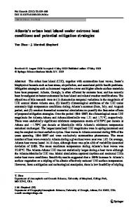
Urban Heat Island Simulations in Guangzhou

sustainability Article

Urban Heat Island Simulations in Guangzhou, China, Using the Coupled WRF/UCM Model with a Land Use Map Extracted from Remote Sensing Data Guang Chen 1 , Lihua Zhao 1, * and Akashi Mochida 2 1 2

*

Building Environment and Energy Laboratory (BEEL), State Key Laboratory of Subtropical Building Science, South China University of Technology, Guangzhou 510641, China; [email protected] Department of Architecture and Building Science, Graduate School of Engineering, Tohoku University, Sendai 980-8579, Japan; [email protected] Correspondence: [email protected]; Tel.: +86-20-8711-2275

Academic Editors: Constantinos Cartalis and Matheos Santamouris Received: 5 May 2016; Accepted: 30 June 2016; Published: 5 July 2016

Abstract: The Weather Research and Forecasting (WRF) model coupled with an Urban Canopy Model (UCM) was used for studying urban environmental issues. Because land use data employed in the WRF model do not agree with the current situation around Guangzhou, China, the performance of WRF/UCM with new land-use data extracted from Remote Sensing (RS) data was evaluated in early August 2012. Results from simulations reveal that experiments with the extracted data are capable of reasonable reproductions of the majority of the observed temporal characteristics of the 2-m temperature, and can capture the characteristics of Urban Heat Island (UHI). The “UCM_12” simulation, which employed the extracted land-use data with the WRF/UCM model, provided the best reproduction of the 2-m temperature data evolution and the smallest minimum absolute average error when compared with the other two experiments without coupled UCM. The contributions of various factors to the UHI effect were analyzed by comparing the energy equilibrium processes of “UCM_12” in urban and suburban areas. Analysis revealed that energy equilibrium processes with new land use data can explain the diurnal character of the UHI intensity variation. Furthermore, land use data extracted from RS can be used to simulate the UHI. Keywords: WRF/UCM model; remote sensing; numerical simulation; urban heat island

1. Introduction Urbanization is a population shift from rural to urban areas, and also covers the ways in which society adapts to this change. It predominantly results in land use and land cover changes and increased building density, both horizontally and vertically, in urban areas. Land use and land cover changes associated with urbanization can have a considerable impact on urban climate [1]. One phenomenon is a consistent rise in temperature in the urban atmosphere caused by the land use changes, and the accompanying effects on the physical processes governing energy, momentum, and matter exchanges between the land surface and the atmosphere [2,3]. Guangzhou, the capital and largest city of Guangdong Province and the third largest city in China, is undergoing rapid and widespread urbanization and a deterioration of the urban environment caused by Urban Heat Island (UHI). The Weather Research and Forecasting (WRF) model, coupled with an Urban Canopy Model (UCM), was developed as a community tool for studying urban environmental issues [4,5]. The coupled WRF/UCM modeling system has been applied to many regions, such as Houston, USA [6], Nanjing, China [7], and New York, USA [8], and its performance has been evaluated against observations.

Sustainability 2016, 8, 628; doi:10.3390/su8070628

www.mdpi.com/journal/sustainability

Sustainability 2016, 8, 628

2 of 14

Many studies have performed simulations using land use data from different years with the single-layer urban canopy model in the Noah land surface model to demonstrate that urban development and the accompanying land use changes can make a significant contribution to extreme heat events [9–12]. However, the default data (U.S. Geological Survey (USGS) land use) employed in the WRF model are based on the NationalOceanic and Atmospheric Administration (NOAA) 1-km Advanced Very High Resolution Radiometer (AVHRR) data obtained from 1992 to 1993. Owing to the rapid urban expansion in the past decade in China, the USGS data are considered outdated. Numerical simulations in Guangzhou [9] and Chengdu [13] with the new land use data reproduced better 2-m temperature evolution data with a smaller minimum absolute average error compared with results obtained using the default USGS land use data in the WRF model. Versions of the WRF model after version 3.1 provide an alternative land use dataset based on the Moderate Resolution Imaging Spectroradiometer (MODIS) 2001 satellite products. Implementation of MODIS data results in better performance of the coupled WRF/UCM modeling system, although the urban area in MODIS also falls short of reality because of fast urbanization [14]. The diurnal variations of UHI intensity and the spatial distribution of the UHI effect in Beijing have been reproduced well by the WRF/UCM with MODIS data [15]. The simulation results with MODIS data improved predictions of the accumulated rainfall when compared with the simulation performed using USGS data [16]. Numerical simulations of Taiwan showed that results obtained using MODIS land use data are in better agreement with the observed data than those obtained using USGS data, although MODIS land use data overestimated the urban area [17]. When compared with observational data, numerical simulations in Guangzhou [18] showed improved accuracy using MODIS data compared with USGS data, but poorer accuracy than that obtained using land use data extracted from the Landsat-7 remote sensing dataset. The effect of urbanization on the weather and climate in Hangzhou were investigated using the coupled WRF/UCM model with updated land use data, and the research showed that updated land use data can reproduce the local climate accurately, and that urban land use has a significant impact on the simulated UHI effect [19]. In this study, the land-use data were extracted from the remote sensing dataset of Landsat-7 using a previous research [20] method and then up-to-date extracted land-use data classified as urban land cover were divided into three urban subcategories by satellite-measured night time light data and the normalized difference vegetation index dataset. The mesoscale coupled WRF/UCM model with different land-use data are used to simulate the formation of high-temperature synoptic conditions in the area of Guangzhou in early August 2012. The aim of this research is to demonstrate that, when using the extracted and up-to-date urban land use data from a remote sensing dataset, the WRF/UCM modeling system provides a more accurate simulation of urban temperatures and the UHI effect in Guangzhou. Furthermore, the study aims to simulate the formation of high-temperature synoptic conditions in the area of Guangzhou, and to investigate the properties of coupled WRF/UCM model and their effects on the UHI simulations. 2. Data Sources and Methodology 2.1. Study Area The study area is located in Guangzhou, south China, with a population of 12.78 million as of the 2010 census. Located in the south-central portion of Guangdong, Guangzhou spans between 112˝ 571 and 114˝ 031 E longitudes, and 22˝ 261 and 23˝ 561 N latitudes. Located just south of the Tropic of Cancer, Guangzhou has a humid subtropical climate that is influenced by the East Asian monsoon. Summers are wet with high temperatures, and high heat index. The hottest period in summer usually lasts from 11 July to 20 August, with an average period of 41 days. The mean annual temperature in the city is 22.3 ˝ C, with monthly daily averages ranging from 12.3 ˝ C in January to 28.4 ˝ C in July. Guangzhou is expanding at a very high speed. Statistical data from the China City Statistical Yearbook show that the built-up area in Guangzhou city has increased more than 4 times since the year 2000, which is much faster than the average expansion pace in China. Such tremendous urban


3 of 14


3 of 15

expansion accompanied with increasing built-up areas and human activities causes year 2000, which is much faster than the average expansion paceintensifying in China. Such tremendous urban remarkable modifications of the underlying surface properties, thereby significantly enhancing expansion accompanied with increasing built-up areas and intensifying human activities causes the UHI remarkable effect [17]. modifications Previous studies show that thesurface UHI effect noticeably contributes toenhancing regional warming of the underlying properties, thereby significantly the UHI effect area [17].[21]. Previous studiesarea show that the effect noticeably contributes to regional in Guangzhou This study includes theUHI seven main districts of Guangzhou, all of which warming in Guangzhou [21]. This study area includes the seven main districts of Guangzhou, are undergoing rapid urbanarea expansion. all of which are undergoing rapid urban expansion.

2.2. Model Configuration 2.2. Model Configuration

The WRF version 3.2 model, coupled with a sophisticated single-layer UCM, was used in this The WRF version 3.2 model, coupled with a sophisticated single-layer UCM, was used in this study [5]. Three one-way nested domains with 72 ˆ 72, 101 ˆ 101, and 121 ˆ 121 grid points, and grid study [5]. Three one-way nested domains with 72 × 72, 101 × 101, and 121 × 121 grid points, and grid spacings of 25, 5, and 1 km, respectively, were used (Figure 1). The coordinate of the domain’s center spacings of 25, 5, and 1 km, respectively, were used (Figure 1). The coordinate of the domain’s center 1 5711 N by 113˝ 311 811 E. The largest domain (Domain 1) covers most of southern China and the is 22˝is622°6′57’’N by 113°31′8’’E. The largest domain (Domain 1) covers most of southern China and the second domain covers thethe whole area.The Themain main districts of Guangzhou are covered second domain covers wholeGuangdong Guangdong area. districts of Guangzhou are covered by by Domain 3. The integration starts on 20 20July July2012 2012forfor a period of one month. Domain 3. The integration startsatat0:00 0:00 GMT GMT on a period of one month. Four Four days days fromfrom 1 August to 4toAugust were selected performanceofof WRF/UCM different 1 August 4 August were selectedto toevaluate evaluate performance thethe WRF/UCM withwith different land-use data. land-use data.

Figure The three domains used for the for numerical simulation and the location of comparison Figure 1. 1.The threenested nested domains used the numerical simulation and the location of points. comparison points.

The parameterization schemes used in our simulation are listed in Table 1, including long- and The parameterization schemesplanetary used in our simulation are listed land in Table 1, including short-wave radiation processes, boundary layer processes, surface processes, longprocesses, processes, etc. In the WRF model, aboundary single-layerlayer UCMprocesses, was implemented in the NOAH and microphysical short-wave radiation planetary land surface processes, land surface model to account for the thermal and dynamic effects of urban buildings, including microphysical processes, etc. In the WRF model, a single-layer UCM was implemented in thethe NOAH trapping of radiation within the urban canopy. The UCM standard values for heat capacity, land surface model to account for the thermal and dynamic effects of urban buildings, including conductivity, albedo, and emissivity roughness lengthThe for heat andstandard momentum of roof, the trapping of radiation within the urban canopy. UCM values for road, heat and capacity, wall surfaces were employed [4,22]. Initial and lateral boundary conditions were taken from the conductivity, albedo, and emissivity roughness length for heat and momentum of roof, road, and wall National Centers for Environmental Prediction (NCEP) Global Forecast System Final Analyses surfaces were employed [4,22]. Initial and lateral boundary conditions were taken from the National (horizontal resolution of 1° × 1°) with 6-h intervals.

Centers for Environmental Prediction (NCEP) Global Forecast System Final Analyses (horizontal resolution of 1˝ ˆ 1˝ ) with 6-h intervals. Table 1. WRF configurations. Simulation Time

20 July 2012 00:00–20 August 2012 00:00 (GMT) Table 1. WRF configurations. National Centers for Environmental Prediction Final Operational Global Meteorological data Analysis data Simulation Time 20 Julytransfer 2012 00:00–20 August long-wave 2012 00:00radiation (GMT) scheme Long-wave radiation Rapid radiative model (RRTM) Short-wavedata radiationNational Centers for Environmental Dudhia short-wave radiation scheme Meteorological Prediction Final Operational Global Analysis data Surface layer Monin–Obukhov Long-wave radiation Rapid radiative transfer model (RRTM)scheme long-wave radiation scheme Land surface Noah land-surface model+ single-layer Urban scheme Canopy Model (UCM) Short-wave radiation Dudhia short-wave radiation Kain–Fritsch (new Eta) scheme SurfaceCumulus layer Monin–Obukhov scheme Land surface radiation Noah land-surface model+ Dudhia single-layer Urban Canopy Model (UCM) Short-wave scheme

Cumulus Short-wave radiation Micro-physics Boundary layer

Kain–Fritsch (new Eta) scheme Dudhia scheme WRF Double-Moment 6-class Yonsei University (YSU) boundary layer scheme


4 of 14

2.3. Updated Land Use Data To derive and classify each land use class from the Landsat-7 ETM+ images, a supervised classification with the maximum likelihood method, which is the same method as the previous research [20], was only applied to the Domain 3. Supervised classification is a procedure most often used for quantitative analysis of remote sensing image data. It is based on using suitable algorithms to label the pixels in an image as representing particular ground cover classes [23]. The extracted land use classes are essentially consistent with the ones defined from MODIS land use classes of forest, grassland, wetland, cropland, urban, barren land, and water. These land use data are almost the same as the previous research result, here named RS_12 [20]. There is only one urban land category in RS_12 and thus these data cannot reproduce urban effects on local climate caused by heterogeneity in an urban area. A human settlement index (HSI) [24], based on satellite-measured nighttime light imagery and the normalized difference vegetation index (NDVI), was used to divide the extracted urban land cover into three urban subcategories: commercial/industrial/transportation (CIT), high-intensity residential (HIR), and low-intensity residential (LIR). HSI data were obtained from a combination of nighttime light imagery and the normalized difference vegetation index (NDVI) [24], as expressed in Equation (1). HSI “

p1 ´ NDVImax q ` OLSnor 1 ´ OLSnor ` NDVImax ` NDVImax ˆ OLSnor

(1)

where OLSnor is the normalized value of the 2012 Defense Meteorological Satellite Program/Operational Linescan System (DMSP/OLS) image [25,26], expressed by Equation (2). A threshold of 23 was selected to minimize the effects of blooming, a phenomenon observed in DMSP/OLS nighttime imagery. OLSmax is the maximum value in the 2012 DMSP/OLS nighttime light image. OLSnor “

pOLS ´ 23q pOLSmax ´ 23q

(2)

To separate human settlements from bare land effectively, and to remove the effect of cloud contamination, 2012 multi-temporal SPOT NDVI images at a resolution of 1 km ˆ 1 km were used to generate a new NDVI composite index, as shown in Equation (3) [27]. NDV Imax “ MAX pNDVI1, NDVI2, . . . , NDVI23q

(3)

HSI values were used to classify urban land in Guangzhou into the following subcategories: (1) pixels with HSI values ě80th percentile, represented as CIT areas; (2) pixels with HSI values between the 30th and the 80th percentiles, represented as HIR areas; and (3) pixels with HSI values ď30th percentile, represented as LIR areas. The extracted urban land use data were classified into the three urban land cover categories to represent up-to-date urbanization conditions in Guangzhou. These Landsat-7 extracted and then enhanced land use data, named UCM_12, are shown in Figure 2a and the default Modis land use data are shown in Figure 2b. The area in Figure 2 indicates the square in Domain 3. 2.4. Numerical Experiments To understand how well the WRF/UCM simulates the UHI effect in urban environments, three numerical experiments were designed to run with or without the UCM model, and using either the MODIS data or the extracted land use data (Table 2). Sensitivity experiments were conducted as follows: (1) MODIS experiment, integrated solely by the WRF model not coupled with UCM and based on the MODIS land use data, the detailed land use map is shown in Figure 2b; (2) RS_12 experiment, also integrated without UCM and based on the Landsat-7 extracted land use data for 2012; and (3) an experiment based on the enhancement of the extracted land use data from Landsat-7 with HSI and coupled with the UCM model. The physics schemes remained the same for all runs.


5 of 15

Landsat-7 Sustainability 2016,with 8, 628HSI and coupled with the UCM model. The physics schemes remained the same for5 of 14 all runs.

(a) Evergreenneedle-leaf forest Shrubland Urban and built-up CIT

(b) Evergreen broad-leaf forest Permanent wetlands Barren/sparselyvegetated HIR

Mixed forests Croplands Water LIR

Figure 2. Types of land use data in Domain 3: (a) UCM_12, enhancement of the extracted land use

Figure 2. Types of land use data in Domain 3: (a) UCM_12, enhancement of the extracted land use data data from Landsat-7 with HIS; and (b) Modis, default land use data in WRF. from Landsat-7 with HIS; and (b) Modis, default land use data in WRF. Table 2. Experiment design.

Experiments UCM Modis No Experiments UCM RS_12 No Modis No UCM_12 Yes RS_12 No UCM_12 Yes 2.5. Observational Data

Table 2. Experiment design. Land Use MODIS Land Use Extracted from Landsat-7 RS data MODIS Enhancement of the extracted land use data from Landsat-7 by HSI Extracted from Landsat-7 RS data Enhancement of the extracted land use data from Landsat-7 by HSI

The simulation lasts for one month, as obtaining long time data to evaluate performance of the 2.5. Observational Data WRF/UCM and the land use data is better. Only four days of climate data from 1 August 0:00 (GMT)

The simulation for onewere month, as obtaining long timeMeteorological data to evaluate performance to 4 August 24:00 lasts (GMT) 2012 acquired from the Guangzhou Bureau. The first of two days were anduse high-temperature whereas and data cloudy weather was 0:00 the WRF/UCM andsunny the land data is better. weather, Only four days ofrainy climate from 1 August observed on the last two days. The observational data were gathered from four weather stations (GMT) to 4 August 24:00 (GMT) 2012 were acquired from the Guangzhou Meteorological Bureau. (onetwo in adays suburban area, and in urban areas)weather, in Domain 3. Therainy suburban weatherweather station was The first were sunny andthree high-temperature whereas and cloudy (suburban point in Figure 1) is located on an elevation in the mountainous and hilly terrain far observed on the last two days. The observational data were gathered from four weather stations (one away from the downtown of Guangzhou, such that there are no tall buildings and medium-sized in a suburban area, and three in urban areas) in Domain 3. The suburban weather station (suburban enterprises within 3 km, and the station is not shaded. The other three weather stations (Points 1–3 pointininFigure Figure1)1) locatedinon elevation in the hilly terrain away from the areislocated thean urban area. The areamountainous around Point 1and experiences rapidfar urbanization, downtown of its Guangzhou, such that there no tallthe buildings andextracted medium-sized and thus representation greatly differsare between MODIS and land useenterprises map. Pointswithin 2 3 km,and and3the Thetown. otherPoints three 1weather stations (Points 1–3points in Figure 1) model are located arestation locatedisinnot theshaded. old down and 2 were representative for the in theevaluation. urban area.Hourly The area around Point 1 experiences urbanization, andinvestigate thus its representation temperature and wind velocity rapid data were collected to the UHI characteristics and the performance of the WRF/UCM model with the extracted land use data. greatly differs between the MODIS and extracted land use map. Points 2 and 3 are located in the old down town. Points 1 and 2 were representative points for the model evaluation. Hourly temperature 3. Simulation Analysis and wind velocity data were collected to investigate the UHI characteristics and the performance of the WRF/UCM model with extracted land use data. 3.1. Air Temperature at 2-mthe Height To investigate the performance of the WRF/UCM model with the extracted land use data, we 3. Simulation Analysis compared the results of the three experiments with the 2-m temperature data observed at the

3.1. Air Temperature at 2-m Height To investigate the performance of the WRF/UCM model with the extracted land use data, we compared the results of the three experiments with the 2-m temperature data observed at the automatic weather stations. Figure 3a presents the observed and modeled air temperature at 2-m height lasting 20 days from 20 July to 9 August in the suburban area, and the four-day comparison from 1 August to 4 August was analyzed in the urban areas (Figure 3b).



6 of 15

6 of 14

automatic weather stations. Figure 3a presents the observed and modeled air temperature at 2-m

Fromheight Figure 3a, it20can befrom found thattothe modeled temperature cycles are generally lasting days 20 July 9 August in thedaily suburban area, and the four-day comparison consistent with the observational on sunny and hot days, but vary in magnitude on rainy days. The same from 1 August todata 4 August was analyzed in the urban areas (Figure 3b). FrombeFigure can be 3b: found the modeled dailybetter temperature cycles are generally characteristic can found3a,initFigure all that models performed on 1 and 2 August than on 3 and consistent with the observational data on sunny and hot days, but vary in magnitude on rainy days. 4 August because of the rainy and cloudy weather seen on the latter two days. All of the experimental The same characteristic can be found in Figure 3b: all models performed better on 1 and 2 August schemes showed variation ofrainy temperature in urban suburban with than on 3 the and 4diurnal August because of the and cloudy weather seenand on the latter two areas, days. Allthough of the experimental showed thefrom diurnal of experiment temperature in urban and than suburban varying magnitudes. Theschemes air temperature thevariation MODIS was lower the observed areas, varying magnitudes. The air station, temperature the MODIS data during thethough periodwith 0:00–12:00 at the suburban butfrom the RS_12 andexperiment UCM_12was experiments lower than the observed data during the period 0:00–12:00 at the suburban station, but the RS_12 gave lower temperatures from 06:00–12:00. In Figure 3b, all the modeled air temperatures were higher and UCM_12 experiments gave lower temperatures from 06:00–12:00. In Figure 3b, all the modeled than the observed data, and a good fit for the maximum temperature between air temperatures were there higher was than the observed data, and there was a air good fit for the maximum air the three temperature the three the observed data for 1 and 2 August. experiments and the between observed data experiments for 1 and 2and August.

Temperature (°C)

OBS

Modis

RS_12

UCM_12

38 36 34 32 30 28 26 24 Time

Temperature (°C)

(a) OBS

38 36 34 32 30 28 26

Modis

RS_12

UCM_12

Time (b) Figure 3. Comparison of the air temperature at 2-m height simulated in the three experiments with

Figure 3. Comparison of the air (OBS): temperature at 2-m height simulated the observed temperature (a) Suburban station; and (b) Point in 1. the three experiments with the observed temperature (OBS): (a) Suburban station; and (b) Point 1. The simulated and observed daily mean (T2M), maximum (T2MAX), and minimum (T2MIN) 2-m air temperatures are shown in Table 3. In general, the UCM_12 experiment efficiently The simulated anddaily observed daily mean (T2M), maximum (T2MAX), and minimum (T2MIN) 2-m simulated the variations in near-surface air temperature, and the RS_12 results were better temperatures are shown Table 3. In the UCM_12 experiment efficiently simulated the than the MODIS on thein near-surface air general, temperature simulation results.

air daily variations in near-surface air temperature, and the RS_12 results were better than the MODIS on Table 3. Comparison of the simulated and observed 2-m temperatures (T2). the near-surface air temperature simulation results. Suburban Urban * OBS MODIS RS_12 UCM_12 OBS MODIS RS_12 UCM_12 Table 3. Comparison of the simulated and observed 2-m temperatures (T2). T2M (°C) 30.4 31.8 31.3 31.2 32.8 34.3 33.6 33.4 T2MAX (°C) 37.0 36.8 36.8 36.6 37.5 38.1 37.8 37.3 Suburban Urban *28.9 T2MIN (°C) 26.6 27.9 27.1 26.7 28.0 30.2 29.0

OBS (˝ C)

T2M T2MAX (˝ C) T2MIN (˝ C)

30.4 37.0 26.6

average results over 3 urban points. MODIS MODIS *: TheRS_12 UCM_12 OBS

31.8 36.8 27.9

31.3 36.8 27.1

31.2 36.6 26.7

32.8 37.5 28.0

34.3 38.1 30.2

RS_12

UCM_12

33.6 37.8 29.0

33.4 37.3 28.9

*: The average results over 3 urban points.

Willmott suggested using the root mean square error (RMSE), systematic (RMSES ) and unsystematic (RMSEU ) errors, and an index of agreement d to evaluate the simulation performance [28]. The index of agreement d can be interpreted as a measure of how error-free a model predicts a variable. The RMSE summarizes the magnitude of the average difference between observation and prediction.


7 of 14

Systematic errors, described by RMSES , result from causes which occur consistently. RMSEU gives information about unsystematic errors, which consist of a number of small effects are positive and some are negative in terms of affecting the final output value. The good model therefore has a systematic difference of zero while the unsystematic difference should approach the RMSE. The d value of 1.0 indicates perfect agreement between observation and prediction. The d can be calculated by Equation (4) [28,29]. řN 2 1 pPi ´ Oi q (4) d “ 1 ´ ř i“`ˇ ˇ ˇ ˇ ˘ , p0 ď d ď 1q N ˇ P1 ˇ ` ˇO1 ˇ 2 i “1

i

i

where Pi1 “ Pi ´ O, Oi1 “ Oi ´ O. O is the average of the observational data. The index of agreement d describes how accurately a model predicts a variable. When d value is equal to 1.0, it indicates perfect prediction for the variable. The difference measures for the four comparison points 2-m temperature are summarized in Table 4. The RMSE for the three simulations at the four weather stations ranged from 1.41 to 2.86 ˝ C. Additionally, the systematic errors (RMSES ) were comparatively small and the unsystematic errors (RMSEU ) approached the RMSE in UCM_12, indicating that the UCM_12 experiment fits the criteria of the systematic error. The d values for all of the simulations at the four stations ranged from 0.74 to 0.95, suggesting that all three experiments provided a reasonable approximation of the observed data. Comparing the d values for the three simulations for each point, the value at UCM_12 is highest, followed by the RS_12 d value, which is in turn larger than the MODIS d value. This suggests that the extracted land use data used in WRF/UCM model provide the best reproduction of temperature variations among the three simulations in both suburban and urban areas. Additionally, the results show that the extracted land use data provided a better simulation than the MODIS data. Table 4. Quantitative evaluation of three cases’ performance on temperature compared with observed data. MODIS

Comparison Points Suburban point Point 1 Point 2 Point 3

d

RMSEs

RMSEu

RMSE

0.79 0.82 0.88 0.74

1.48 2.00 0.60 2.37

1.88 1.42 1.47 1.60

2.40 2.45 1.59 2.86

RS_12

Suburban point Point 1 Point 2 Point 3

d

RMSEs

RMSEu

RMSE

0.86 0.86 0.90 0.94

1.03 1.70 0.34 2.26

1.72 1.33 1.37 1.45

2.00 2.15 1.41 2.69

UCM_12


d

RMSEs

RMSEu

RMSE

0.89 0.90 0.93 0.95

1.03 1.46 0.29 2.10

1.73 1.38 1.51 1.69

2.01 2.02 1.53 2.69

3.2. Urban Heat Island Intensity (UHII) By comparing the results of the three numerical experiments, their ability to simulate the urban heat island effect can be examined. Figure 4 presents the evolution of the urban heat island intensity (UHII) as simulated by the three experiments. The intensity of the heat island is calculated as the difference of temperature between urban Point 1 and the suburban point at 2-m height. As shown

the other experiments at other times. The maximum UHII and the average local UHII reflect the average difference over the whole day, and were selected to analyze the UHI effect. Modeled and observed values of maximum UHII at Point 1 and Point 2 are compared in Figure 5a,b, respectively. At Point 1, the RS_12 and UCM_12 results have better correspondence to the Sustainability 2016, 8, 628 8 of 14 observations than the MODIS results. The UCM_12 experiment did not show a noticeably better Sustainability 2016, 8, 628the simulations despite the implementation of the coupled WRF/UCM8model. of 15 performance among Point 2, although UCM_12 experiment showed a midday, higher maximum UHII, there is still a large with by theAtobservations, the the UHII gradually increases after reaching night, By comparing the results of the three numerical experiments, their abilityatomaximum simulate theaturban deviation from the observations. On 3 August, ˝none of the experiments agreed with the heat island effect can be examined.of Figure 4 presents of the urban heat island intensity in the a maximum temperature difference more than 5 the C.evolution The UHII then gradually decreases observations, predominantly because of the rainy weather. (UHII) simulated negative by the three The intensity of the heat island is calculated as the morning, evenasbecoming at experiments. noon.

Temperature (°C)

difference of temperature between urban Point 1 and the suburban point at 2-m height. As shown by the observations, the UHII gradually increases after midday, a maximumUCM_12 at night, with Obs Modis reaching RS_12 a6 maximum temperature difference of more than 5 °C. The UHII then gradually decreases in the morning, even becoming negative at noon. 4 All experiments plausibly reproduce the characteristics of UHII evolution, except for on 3 August, when the negative UHII is weakly reproduced and its overall variation is underestimated. 2 UCM_12 produces a better reproduction of the UHII at peak values, but a poorer reproduction than the 0 other experiments at other times. The maximum UHII and the average local UHII reflect the average difference over the whole Time day, and were selected to analyze the UHI effect. -2 Modeled and observed values of maximum UHII at Point 1 and Point 2 are compared in Figure FigureAt4.Point Heat 1, island intensity the different experiments atcorrespondence Point 1. 5a,b, respectively. the RS_12 andof results have better to the Figure 4. Heat island intensity ofUCM_12 the different experiments at Point 1. observations than the MODIS results. The UCM_12 experiment did not show a noticeably better among the simulations despite the implementation of the coupled WRF/UCM model. Allperformance experiments reproduce the characteristics of UHII evolution, except for on 3 August, OBS plausibly MODIS RS_12 UCM_12 OBSmaximum MODIS UHII, RS_12 At6.0 Point 2, although the UCM_12 experiment showed a higher thereUCM_12 is still a large when the negative UHII is weakly reproduced and8.0 its overall variation is underestimated. UCM_12 deviation from the observations. On 3 August, none of the experiments agreed with the produces a better reproduction the UHII atrainy peakweather. values, but a poorer reproduction than the other 6.0 observations, predominantlyofbecause of the 4.0

Temperature (°C)

experiments at other times. 4.0 2.0 The maximum UHII and the average localObs UHII2.0 reflect over the whole day, Modisthe average RS_12difference UCM_12 6 and were0.0 selected to analyze the UHI effect. 0.0 Modeled and observed maximum UHIIAug.1st at PointAug.2nd 1 and Point 2 are compared in Aug.1st Aug.2nd values Aug.3rd of Aug.4th 4 Aug.3rd Aug.4th Figure 5a,b, respectively. At Point 1, the RS_12 and UCM_12 results have better correspondence (a) (b) 2 to the observations than the MODIS results. The UCM_12 experiment did not show a noticeably better Figure 5. The Maximum UHII: (a) Point 1; and (b) Point 2. performance 0 among the simulations despite the implementation of the coupled WRF/UCM model. At Point 2,The although the UCM_12 experiment showed a higher maximum UHII, there isTime still a large -2 average local UHII were calculate by Equation (5), deviation from the observations. On 3 August, none of the 𝑡1 experiments agreed with the observations, 𝑡1 ∫𝑡0 𝑇𝑢 𝑑𝑡 − ∫𝑡0 𝑇𝑟 𝑑𝑡 predominantly because of the rainy weather. 𝑈𝐻𝐼𝐼 = (5) Figure 4. Heat island intensity of the different experiments at Point 1. avg 𝑡1

∫𝑡0 𝑑𝑡

OBS for MODIS RS_122-mUCM_12 where, Tu stands the hourly height temperature in OBS the urban area,RS_12 Tr stands for the hourly MODIS UCM_12 6.0 temperature in the suburban area, t 8.0 2-m height 0 stands for initial time of the simulation, and t 1 6.0 stands 4.0 for end time of the simulation.

4.0

2.0

2.0

0.0

0.0

Aug.1st Aug.2nd Aug.3rd Aug.4th

Aug.1st

(a)

Aug.2nd

Aug.3rd

Aug.4th

(b)

Figure 5. The Maximum UHII: (a) Point 1; and (b) Point 2.

Figure 5. The Maximum UHII: (a) Point 1; and (b) Point 2. The average local UHII were calculate by Equation (5), 𝑡1 𝑡1 The average local UHII were calculate by Equation (5), ∫ 𝑇 𝑑𝑡 − ∫ 𝑇 𝑑𝑡

𝑈𝐻𝐼𝐼avg =

𝑡0

r t1 t0

𝑢

𝑡1

𝑡0

𝑟

∫𝑡0 𝑑𝑡r t1

Tu dt ´

t0

Tr dt

(5)

Iavg “temperature r t1 in the urban area, Tr stands for the hourly where, Tu stands for the hourlyUH 2-mIheight t0 dt 2-m height temperature in the suburban area, t 0 stands for initial time of the simulation, and t1 stands for end time of the simulation.

(5)

where, Tu stands for the hourly 2-m height temperature in the urban area, Tr stands for the hourly 2-m height temperature in the suburban area, t0 stands for initial time of the simulation, and t1 stands for end time of the simulation. The average local UHII for all experiments and the observation data at Point 1 and Point 2 are shown in Figure 6a,b. The daytime was constrained between 8:00 and 20:00 and the rest was considered as nighttime. All experiments have a better agreement with the observations and represent larger magnitudes of average local UHII at Point 2 than at Point 1. All experiments underestimate both


9 of 15

The average local UHII for all experiments and the observation data at Point 1 and Point 2 are Sustainability 2016,in8, Figure 628 9 of 14 shown 6a,b. The daytime was constrained between 8:00 and 20:00 and the rest was

considered as nighttime. All experiments have a better agreement with the observations and Sustainability 2016, 8, 628 9 of 15 represent larger magnitudes of average local UHII at Point 2 than at Point 1. All experiments day- and nighttime UHII. In urban areas, the UCM_12 experiment produces poor statistical scores for underestimate both day- and nighttime UHII. In urban areas, the UCM_12 experiment produces The average local UHII for all experiments and the observation data at Point 1 and Point 2 are the average daytime local UHII, but better ones for the average nighttime local UHII. The UCM_12 poor statistical scores for the average daytime local UHII, but better ones for the average nighttime shown in Figure 6a,b. The daytime was constrained between 8:00 and 20:00 and the rest was local UHII. The UCM_12 experiment produces highest average nighttime local is UHII, experiment produces the highest nighttime UHII, although stillalthough lower considered as nighttime. Allaverage experiments have the a local better agreement with the the value observations and than the value is still lower than the observed one. the observed one. represent larger magnitudes of average local UHII at Point 2 than at Point 1. All experiments underestimate both day- and nighttime UHII. In urban areas, the UCM_12 experiment produces Average UHII of UHII nighttime poor statistical scores for the average daytime local UHII, but better ones forAverage the average 6.0 4.0 Average UHII of day Average UHII of day local UHII. The UCM_12 experiment produces the highest average nighttime local UHII, although Average UHII of night Average UHII of night the value is still lower than the observed one. 4.0

2.0 Average UHII Average UHII of day Average UHII of night

4.0

0.0 OBS

2.0

MODIS

RS_12 UCM_12

2.0

Average of UHII Average UHII of day Average UHII of night

6.0

4.00.0

OBS

MODIS

RS_12

UCM_12

2.0 (a)

0.0 OBS

(b) 0.0 Figure 6. The average local UHII: (a) Point 1; MODIS and (b) Point 2. RS_12 MODIS UCM_12local UHII: (a) OBS Figure 6.RS_12 The average Point 1; and (b) Point 2.

UCM_12

Although the results of the coupled WRF/UCM model do(b)not accurately reproduce the (a)

Although the and results of the coupledunderestimated WRF/UCM model do not accurately observations reveal consistently UHII, they feasibly reflect reproduce the diurnalthe Figure 6. The average local UHII: (a) Point 1; and (b) Point 2. variation ofreveal the UHII. Additionally, the coupled WRF/UCM exhibits better with of observations and consistently underestimated UHII, theymodel feasibly reflect the performance diurnal variation the Additionally, extracted land use data than with the MODIS land use data. the UHII. the coupled WRF/UCM model exhibits better performance with the extracted Although the results of the coupled WRF/UCM model do not accurately reproduce the and the reveal consistently underestimated UHII, they feasibly reflect the diurnal land useobservations data than with MODIS land use data. 3.3. Wind Velocity at 10-m Height variation of the UHII. Additionally, the coupled WRF/UCM model exhibits better performance with

theVelocity extracted use data thanall with landresults use data. 3.3. Wind atland 10-m Height Regarding wind velocity, of the the MODIS simulation were close to the observation data in the

daytime. The observed and simulated wind velocity at 10-m height at the suburban point and Point

Regarding wind velocity, all of the simulation results were close to the observation data in the 3.3. Wind Velocity at 10-m Height 1 are shown in Figure 7a,b, respectively. In general, wind velocity simulated in all three experiments daytime. The observed and simulated velocity results at 10-m height the observation suburban pointinand 1 Regarding wind all ofwind thetrends simulation were close at to the Point is overestimated, andvelocity, the distribution of all the experiments arethe similar when data comparing the are shown in Figure 7a,b, respectively. In general, wind velocity simulated in all three experiments daytime. Theand observed and simulated wind velocity 10-m modeled height at the point andvelocity Point is simulations observations. For the urban area,atboth andsuburban observed wind is overestimated, the distribution trends oftoallthe the experiments are similar when comparing 1 are shown in Figure 7a,b, respectively. In general, wind velocity simulated in all It three experiments lower in theand nighttime, which corresponds changes in UHI intensity. is believed that thethe is overestimated, and theofdistribution trends allboth the experiments are nighttime similar when comparing the simulations and observations. For the urban modeled observed wind velocity lower strong thermal stability the surface layerarea, isofthe primary reasonand for enhancement of is UHI. and For to thewind urban area,isboth modeled and observed wind velocity is strong Itsimulations should also be observations. noted that surface speed generally reduced in a stable surface All in the nighttime, which corresponds the changes in UHI intensity. It is believed thatlayer. the lower in the have nighttime, corresponds to the changes UHI intensity. Even It is believed that coupled the largewhich magnitudes compared with for theinnighttime observations. using thermalexperiments stability of the surface layer is the primary reason enhancement of the UHI. It should strong thermal stability of the surface layer is the primary reason for nighttime enhancement of UHI. model, thewind influence of is thegenerally buildingsreduced on the wind environment cannot be reproduced. also beWRF/UCM noted that surface speed in a stable surface layer. All experiments It should also be noted that surface wind speed is generally reduced in a stable surface layer. All have large magnitudes with the observations. using theEven coupled experiments have compared large magnitudes compared with theEven observations. usingWRF/UCM the coupled model, OBSon the wind Modis RS_12 UCM_12 WRF/UCM model, the influence the buildings environment cannot be reproduced. the influence of buildings on theofwind environment cannot be reproduced. 6.0the Wind velocity Wind velocity （m/s/）（m/s/）

5.0 4.0 3.0 6.0 2.0 5.0 4.0 1.0 3.0 0.0

OBS

Modis

RS_12

UCM_12

2.0 1-Aug 6:00 12:00 18:00 2-Aug 6:00 12:00 18:00 3-Aug 6:00 12:00 18:00 4-Aug 6:00 12:00 18:00 Time 1.0 0.0 1-Aug 6:00 12:00 18:00 2-Aug 6:00 12:00 18:00 (a) 3-Aug 6:00 12:00 18:00 4-Aug 6:00 12:00 18:00 Time


10 of 15

Wind velocity （m/s/）

(a)

6.0 5.0 4.0 3.0 2.0 1.0 0.0

OBS

Modis

RS_12

UCM_12

1-Aug 6:00 12:00 18:00 2-Aug 6:00 12:00 18:00 3-Aug 6:00 12:00 18:00 4-Aug 6:00 12:00 18:00 Time

(b) Figure 7. Comparison of the wind velocity at 10-m height simulated in the three experiments with

Figure 7. Comparison of the wind velocity at 10-m height simulated in the three experiments with observations: (a) Suburban station; and (b) Point 1. observations: (a) Suburban station; and (b) Point 1. The difference measures of the modeled wind velocity at 10-m height of four comparison points are summarized in Table 5. The d values for all experiments at the four stations ranged from 0.34 to 0.70, indicating low consistency of simulations with the observed data. At the same time, the systematic errors ( RMSES ) were comparatively small and the unsystematic errors ( RMSEU ) approached the RMSE in UCM_12, indicating better performance of coupled WRF/UCM with extracted land use data compared to other cases, although the improvement is relatively small.


10 of 14

The difference measures of the modeled wind velocity at 10-m height of four comparison points are summarized in Table 5. The d values for all experiments at the four stations ranged from 0.34 to 0.70, indicating low consistency of simulations with the observed data. At the same time, the systematic errors (RMSES ) were comparatively small and the unsystematic errors (RMSEU ) approached the RMSE in UCM_12, indicating better performance of coupled WRF/UCM with extracted land use data compared to other cases, although the improvement is relatively small. Table 5. Quantitative evaluation of three cases’ performance on wind velocity compared with observed data. MODIS

Comparison Points Suburban point Point 1 Point 2 Point 3

d

RMSEs

RMSEu

RMSE

0.64 0.51 0.44 0.43

1.59 1.54 1.42 1.59

1.31 0.78 0.74 0.82

2.06 1.73 1.61 1.79

RS_12


d

RMSEs

RMSEu

RMSE

0.68 0.49 0.34 0.53

1.03 1.65 2.10 1.24

1.72 0.77 0.85 1.45

2.00 1.82 2.27 2.69

UCM_12


d

RMSEs

RMSEu

RMSE

0.70 0.52 0.45 0.50

1.01 1.55 1.42 1.35

1.01 0.64 0.74 0.80

1.47 1.68 1.61 1.57

3.4. Energy Balance Data

Energy Flux （w/m2)

The UHI is mainly determined by the surface energy balance [30], and the contributing factors during land surface energy equilibrium processes on the UHI can be represented in models. To focus on the formation of the UHI on 1 August and to investigate the performance of the UCM in simulating the UHI, the energy equilibrium processes between urban and suburban areas, and between experiments UCM_12 and RS_12, were compared and analyzed. Figure 8 shows the temporal variability of parameters relevant to the land surface energy equilibrium in the urban area during the UCM_12 Sustainability 2016, 8, 628 11 of 15 experiment from 1 August 00:00 (GMT) to 23:00 (GMT). shortwave absorbed

longwave incoming

latent heat flux

ground heat flux

upward heat flux

1200 1000 800 600 400 200 0 -200 -400

Time

Figure 8. Temporal evolution of of parameters to the theland landsurface surface energy equilibrium in the Figure 8. Temporal evolution parametersrelevant relevant to energy equilibrium in the urbanurban area during the UCM_12 experiment on 1 August. area during the UCM_12 experiment on 1 August.

The absorption of solar short-wave radiation is predominantly an energy input, whereas the outputs are latent heat flux and ground heat flux. Long-wave radiation shows weak daily variation (approximately 450 W/m2). Ground heat flux and upward heat flux reach their maximum values of 250 and 340 W/m2, respectively, in the daytime around noon. The latent heat flux only reaches a maximum of 100 W/m2 owing to evaporation, which is absent at night. At night, the ground heat


11 of 14

The absorption of solar short-wave radiation is predominantly an energy input, whereas the outputs are latent heat flux and ground heat flux. Long-wave radiation shows weak daily variation (approximately 450 W/m2 ). Ground heat flux and upward heat flux reach their maximum values of 250 and 340 W/m2 , respectively, in the daytime around noon. The latent heat flux only reaches a maximum of 100 W/m2 owing to evaporation, which is absent at night. At night, the ground heat flux acts as an input, becoming a major source of energy, while the upward heat flux, though much smaller than during the daytime, remains positive as it continues to transfer heat to the atmosphere. The characteristics of these energy equilibrium processes suggest a positive performance when simulating the UHI using the WRF/UCM with the land use data extracted from remote sensing data. Figure 9 presents the differences in the energy equilibrium between Point 1 and the suburban point simulated in the UCM_12 experiment. Urban areas absorb more short-wave radiation than suburban areas, although the difference is small. The diurnal latent heat flux was significantly different between the urban and suburban areas. During the day, the latent heat flux was reduced in urban areas because of the limited vegetation and less evaporation, while it remained small at night. During the day, the upward heat flux was significantly higher in the urban area than in the suburban areas, close to 200 W/m2 . After sunset, the difference in the ground heat flux turns from negative to positive, while that of upward heat flux remained positive. The positive heat fluxes, though small, resulted in aSustainability higher temperature 2016, 8, 628 at night in urban areas than in suburban areas. The WRF model simulation 12 ofof15 UHI with the land use data extracted from remote sensing data can reveal the causes of the UHI. shortwave absorbed

longwave incoming

latent heat flux

ground heat flux

upward heat flux


200 100 0 0:00

4:00

8:00

12:00

16:00

20:00

-100 Time -200 -300 -400

Figure 9. Differences in the energy equilibrium between Point 1 and the suburban point for the Figure 9.simulation. Differences in the energy equilibrium between Point 1 and the suburban point for the UCM_12 UCM_12 simulation.


Figure 10 shows the differences between the individual terms of energy equilibrium between the UCM_12 and RS_12 experiments. The improvement of the simulation performance by the UCM shortwave absorbed longwave incoming upward heat flux model can be illustrated from the difference. The urban latent heat flux is reduced in the daytime when coupled UCM the model in UCM_12, the reduction reaches a maximum of 100 W/m2 . In addition, latent heat flux ground heat flux the UCM_12 simulation suggested a larger diurnally upward heat flux and ground heat flux than 100 the RS_12 simulation. This suggests that the urban canopy model can be used to improve nighttime UHI simulations. 50

0 0:00 -50

-100

4:00

8:00

12:00

16:00

20:00 Time

-400

Figure 9. Differences in the energy equilibrium between Point 1 and the suburban point for the UCM_12 simulation.



12 of 14

shortwave absorbed

longwave incoming

latent heat flux

ground heat flux

upward heat flux

100

50

0 0:00 -50

4:00

8:00

12:00

16:00

20:00 Time

-100

Figure 10. Differences in the energy equilibrium between the UCM_12 and RS_12 simulation.

Figure 10. Differences in the energy equilibrium between the UCM_12 and RS_12 simulation.

4. Summary and Conclusions 4. Summary and Conclusions The thermal environment over Guangzhou from late July to early August 2012 was investigated thermal WRF/UCM environment overSimulation Guangzhou from latewere Julyperformed to earlyusing August was usingThe the coupled model. experiments both2012 the urban investigated the coupled WRF/UCM experiments land use datausing extracted from remote sensing model. datasetsSimulation and the default MODIS were data. performed using both the urban land use data extracted from remote sensing datasets and the default MODIS data. (1) Using the new land use data, the simulated 20 days of daily temperature cycles at the suburban (1) Using the new land use data, the simulated 20 days of daily temperature cycles at the weather station and four days of daily temperature cycles at urban point showed an encouraging suburban weather station and four days of daily temperature cycles at urban point showed an agreement with observations, especially on hot sunny days. UCM_12 simulated maximum diurnal encouraging agreement with observations, especially on hot sunny days. UCM_12 simulated temperatures closer to the observed values than the simulations that excluded the UCM model. maximum diurnal temperatures closer to the observed values than the simulations that The coupled WRF/UCM with the new land use data improved the simulation performance. excluded the UCM model. The coupled WRF/UCM with the new land use data improved the (2) Compared with the maximum UHII and the average local UHII, all of the simulated results simulation performance. reproduced the diurnal characteristics of UHI intensity. Both RS_12 and UCM_12 simulations (2) Compared with the maximum UHII and the average local UHII, all of the simulated results performed better than the default geographic model, although they did not perfectly replicate reproduced the diurnal characteristics of UHI intensity. Both RS_12 and UCM_12 simulations the observations. (3) The modeled wind velocity results were higher than observations. The new land use data produced similar results as the default land use data. For the urban area, all wind velocity simulation results and observations were lower, and the UHII remains high during the nighttime. (4) The UCM_12 experiment successfully reproduced the differences in the energy equilibrium both in the urban and suburban areas. In the urban area, most of the input energy is used in sensible heating, which resulting the higher temperature, can be simulated by the WRF/UCM. The latent heat flux in the urban area is lower than in suburban area because lack of evapotranspiration of water vapor in the urban area. For the nocturnal situation, relatively high minimum temperature is reproduced in the urban owing to the sustained upward ground heat flux heats the atmosphere in the urban area. As changing the land use data can have a significant impact on the WRF/UCM simulation result, this study confirmed that the WRF/UCM model with land use data extracted from a remote sensing dataset can be an effective tool for urban thermal environment analyses. Acknowledgments: This study was supported by the State Key Laboratory of Subtropical Building Science, South China University of Technology, China (Project No. 2015ZC12); the National Natural Science Foundation of China (Project No. 51408303); and the China Scholarship Council Program (No. [2013]3009). Helpful comments from Yufeng Zhang and Xiaoshan Yang were greatly appreciated. Author Contributions: All three authors significantly contributed to the scientific study and writing. Guang Chen and Lihua Zhao contributed to the overall idea, planning, financing, analyzing and writing of the manuscript, and


13 of 14

conceived and designed the simulation. Akashi Mochida contributed to discussions on the land use data issues of this paper and manuscript preparations. Conflicts of Interest: The authors declare no conflict of interest.

Abbreviations The following abbreviations are used in this manuscript: WRF UCM UHI CIT HIR LIR UHII

Weather Research and Forecasting Urban Canopy Model Urban Heat Island Commercial/Industrial/Transportation High-Intensity Residential Low-Intensity Residential Urban Heat Island Intensity

References 1. 2. 3.

4. 5.

6.

7. 8. 9. 10.

11. 12. 13. 14. 15.

Foley, J.A.; DeFries, R.; Asner, G.P.; Barford, C.; Bonan, G.; Carpenter, S.R.; Chapin, F.S.; Coe, M.T.; Daily, G.C.; Gibbs, H.K.; et al. Global consequences of land use. Science 2005, 309, 570–574. [CrossRef] [PubMed] Cotton, W.R.; Pielke, R.A. Human Impacts on Weather and Climate; Cambridge University Press: Cambridge, UK, 2007. Zhang, C.L.; Chen, F.; Miao, S.G.; Li, Q.C.; Xia, X.A.; Xuan, C.Y. Impacts of urban expansion and future green planting on summer precipitation in the Beijing metropolitan area. J. Geophys. Res. Atmos. (1984–2012) 2009. [CrossRef] Kusaka, H.; Kondo, H.; Kikegawa, Y.; Kimura, F. A simple single-layer urban canopy model for atmospheric models: Comparison with multi-layer and slab models. Bound.-Layer Meteorol. 2001, 101, 329–358. [CrossRef] Chen, F.; Kusaka, H.; Bornstein, R.; Ching, J.; Grimmond, C.S.B.; Grossman-Clarke, S.; Loridan, T.; Manning, K.W.; Martilli, A.; Miao, S.; et al. The integrated WRF/urban modelling system: Development, evaluation, and applications to urban environmental problems. Int. J. Climatol. 2011, 31, 273–288. [CrossRef] Chen, F.; Kusaka, H.; Tewari, M.; Bao, J.W.; Hirakuchi, H. Utilizing the coupled WRF/LSM/Urban modeling system with detailed urban classification to simulate the urban heat island phenomena over the Greater Houston area. In Proceedings of the Fifth Symposium on the Urban Environment, Vancouver, BC, Canada, 23–27 August 2004. Yang, B.; Zhang, Y.; Qian, Y. Simulation of urban climate with high-resolution WRF model: A case study in Nanjing, China. Asia-Pac. J. Atmos. Sci. 2012, 48, 227–241. [CrossRef] Holt, T.; Pullen, J. Urban canopy modeling of the New York City metropolitan area: A comparison and validation of single-and multilayer parameterizations. Mon. Weather Rev. 2007, 135, 1906–1930. [CrossRef] Meng, W.; Zhang, Y.-X.; Li, J.-N.; Lin, W.-S.; Dai, G.-F.; Li, H.-H. Application of WRF/UCM in the simulation of a heat wave event and urban heat island around Guangzhou. J. Trop. Meteorol. 2011, 17, 256–265. Grossman-clarke, S.; Zehnder, J.A.; Loridan, T.; Grimmond, C.S.B. Contribution of land use changes to near-surface air temperatures during recent summer extreme heat events in the Phoenix metropolitan area. J. Appl. Meteorol. Climatol. 2010, 49, 1649–1664. [CrossRef] Jiang, X.; Wiedinmyer, C.; Chen, F.; Yang, Z.-L.; Lo, J.C.-F. Predicted impacts of climate and land use change on surface ozone in the Houston, Texas, area. J. Geophys. Res. Atmos. (1984–2012) 2008. [CrossRef] Chen, J.; Li, Q.; Niu, J.; Sun, L. Regional climate change and local urbanization effects on weather variables in Southeast China. Stochast. Environ. Res. Risk Assess. 2011, 25, 555–565. [CrossRef] Xiao, D.; Chen, J.; Chen, Z.; Zhang, B. Effect Simulation of Chengdu Fine Underlying Surface Information on Urban Meteorology. Meteorol. Mon. 2011, 37, 298–308. Kuang, W.; Liu, J.; Zhang, Z.; Lu, D.; Xiang, B. Spatiotemporal dynamics of impervious surface areas across China during the early 21st century. Chin. Sci. Bull. 2013, 58, 1691–1701. [CrossRef] Miao, S.; Chen, F.; Lemone, M.A.; Tewari, M.; Li, Q.; Wang, Y. An Observational and Modeling Study of Characteristics of Urban Heat Island and Boundary Layer Structures in Beijing. J. Appl. Meteorol. Climatol. 2009. [CrossRef]


16.

17.

18.

19. 20. 21. 22.

23.

24. 25. 26. 27. 28. 29. 30.

14 of 14

Lin, C.-Y.; Chen, W.-C.; Chang, P.-L.; Sheng, Y.-F. Impact of the urban heat island effect on precipitation over a complex geographic environment in Northern Taiwan. J. Appl. Meteorol. Climatol. 2011, 50, 339–353. [CrossRef] Cheng, F.-Y.; Hsu, Y.-C.; Lin, P.-L.; Lin, T.H. Investigation of the effects of different land use and land cover patterns on mesoscale meteorological simulations in the Taiwan area. J. Appl. Meteorol. Climatol. 2013, 52, 570–587. [CrossRef] Li, Y.; Okaze, T.; Mochida, A. Prediction of the impacts of urbanization using a new assessment system combining an urban expansion model and WRF-Case study for Guangzhou in China. J. Heat Island Inst. Int. 2014, 9, 133–137. Chen, F.; Yang, X.; Zhu, W. WRF simulations of urban heat island under hot-weather synoptic conditions: The case study of Hangzhou City, China. Atmos. Res. 2014, 138, 364–377. [CrossRef] Li, Y.; Song, Y.H.; Mochida, A.; Okaze, T. WRF Environment Assessment in Guangzhou City with an Extracted Land-use Map from the Remote Sensing Data in 2000 as an Example. J. Harbin Inst. Technol. 2014, 21, 26–32. Cheng, C.K.M.; Chan, J.C.L. Impacts of land use changes and synoptic forcing on the seasonal climate over the Pearl River Delta of China. Atmos. Res. 2012, 60, 25–36. [CrossRef] Kusaka, H.; Kimura, F. Thermal effects of urban canyon structure on the nocturnal heat island: Numerical experiment using a mesoscale model coupled with an urban canopy model. J. Appl. Meteorol. 2004, 43, 1899–1910. [CrossRef] AL-Ahmadi, F.S.; Hames, A.S. Comparison of Four Classification Methods to Extract Land Use and Land Cover from Raw Satellite Images for Some Remote Arid Areas, Kingdom of Saudi Arabia. King Abdul. Univ. 2009, 20, 167–191. [CrossRef] Lu, D.; Tian, H.; Zhou, G.; Ge, H. Regional mapping of human settlements in southeastern China with multisensor remotely sensed data. Remote Sens. Environ. 2008, 112, 3668–3679. [CrossRef] Elvidge, C.D.; Baugh, K.E.; Kihn, E.A.; Kroehl, H.W.; Davis, E.R. Mapping city lights with nighttime data from the DMSP Operational Linescan System. Photogramm. Eng. Remote Sens. 1997, 63, 727–734. Elvidge, C.D.; Baugh, K.E.; Dietz, J.B.; Bland, T.; Sutton, P.C.; Kroehl, H.W. Radiance Calibration of DMSP-OLS Low-Light Imaging Data of Human Settlements. Remote Sens. Environ. 1999, 68, 77–88. [CrossRef] Maisongrande, P.; Duchemin, B.; Dedieu, G. VEGETATION/SPOT: An operational mission for the Earth monitoring; presentation of new standard products. Int. J. Remote Sens. 2004, 25, 9–14. [CrossRef] Willmott, C.J. Some comments on the evaluation of model performance. Bull. Am. Meteorol. Soc. 1982, 63, 1309–1313. [CrossRef] Srunnaa, M.; Sethuraman, S. A statistical evaluation and comparison of coast point source dispersion models. Atmos. Environ. 1986, 20, 301–315. Oke, T.R. The energetic basis of the urban heat island. Quart. J. Royal Meteorol. Soc. 1982, 108, 1–24. [CrossRef] © 2016 by the authors; licensee MDPI, Basel, Switzerland. This article is an open access article distributed under the terms and conditions of the Creative Commons Attribution (CC-BY) license (http://creativecommons.org/licenses/by/4.0/).