Using data-mining techniques for PM10 forecasting in the metropolitan area of Thessaloniki, Greece Fani A. Tzima, Kostas D. Karatzas, Pericles A. Mitkas and Stavros Karathanasis Abstract— Knowledge extraction and acute forecasting are among the most challenging issues concerning the use of computational intelligence (CI) methods in real world applications. Both aspects are essential in cases where decision making is required, especially in domains directly related to the quality of life, like the quality of the atmospheric environment. In the present paper we emphasize on short term Air Quality (AQ) forecasting as a key constituent of every AQ management system, and we apply various CI methods and tools for assessing PM10 concentration values. We report our experimental strategy and preliminary results that reveal interesting interrelations between AQ and various city operations, while performing satisfactory in predicting concentration values.
I. I NTRODUCTION One of the most challenging issues concerning the use of computational intelligence (CI) methods in real world applications is knowledge extraction for the application domain of interest, and acute forecasting. While the former is related to the “creative” collaboration of knowledge domain expertise with appropriate, knowledge mapping, CI methods, the latter is related with the effective selection of parameters of interest. Both aspects are very important when the emphasis is on domains directly related to the quality of life, like the quality of the atmospheric environment, which is generally addressed as the problem of air quality management (AQM). In addition to that, AQM is among the most challenging domains for CI methods and tools, as it deals with: • a problem that has no analytical solution (that of air pollution reduction), as it combines the non-linearity of the physical and chemical atmospheric processes, with optimization problems in relation to human activities and decision making that affect air quality (AQ); • a regulatory framework that dictates the parameters of interest and the ways that they should be assessed; • human perception of the quality of the atmospheric environment, that may not be deterministically linked with the aforementioned parameters; and F. A. Tzima is with the Department of Electrical and Computer Engineering, Aristotle University of Thessaloniki, GR-541 24, Thessaloniki, Greece (phone: +30 2310 996359; fax: +30 2310 996398; email:
[email protected]). K. D. Karatzas is with the Department of Mechanical Engineering, Aristotle University of Thessaloniki, Box 483, GR-541 24 Thessaloniki, Greece (phone/fax: +30 2310 994176; email:
[email protected]) P. A. Mitkas is with the Department of Electrical and Computer Engineering, Aristotle University of Thessaloniki, GR-541 24, Thessaloniki, Greece (phone: +30 2310 996390; fax: +30 2310 996398; email:
[email protected]). S. Karathanasis is with the Directorate of Environment and Land Planning, Region of Central Macedonia, 1 Taki Economidi Str, GR-54008 Thessaloniki, Greece (phone: +30 2310 409261; email:
[email protected])
lack of sufficient data, missing or bad quality of data describing the problem domain. On this basis, the current paper aims at investigating the application of various CI methods for knowledge discovery and parameter forecasting in the domain of AQM, with emphasis on the urban environment (where the majority of the population lives in). •
II. BACKGROUND A. Urban air quality management In the life cycle of environmental information within an urban domain, the environment is the data “generator” per se. However, the existing regulatory (legislative) framework specifies procedures, methods and terms under which environmental monitoring and modeling should take place for regulatory purposes, and defines urban environment management actions by which environmental quality related goals should be reached in an area of interest [1]. Air quality is one of the most advanced environmental fields regarding the legal framework developed in the European Union, the USA, and many other countries. In addition, AQ is among the major themes of environmental interest for the World Health Organization (WHO). The regulatory framework defines alert thresholds and limit values, plus a margin of tolerance, all being unique per pollutant. Each pollutant is monitored with the aid of specialized equipment, producing hourly concentration values. For each pollutant, a different criterion is set by the legislation (and the WHO), concerning the averaging period and the type of exceedances to be used as assessment criteria [2]. In the following, a subset of these pollutants is discussed, to demonstrate the aforementioned differences. • Particulate matter. This is a category of pollutants, which are further classified on the basis of their mean aerodynamic diameter and of the state that they are in. One of the “traditional” ones is PM10 , i.e. particulate matter of solid state and mean diameter in the order of 10µm. This is a pollutant that is directly emitted by combustion processes and by traffic, while in some regions is also produced as the result of mechanical degradation of the road surface and of winter tires. The criterion applied for assessment is the mean 24h averaged concentration, and the limit value used equals 50µg/m3 , not to be exceeded more than 7 times per calendar year. An additional criterion is the mean annual value (20µg/m3 ). Both limit values will be updated in the future.
•
•
Nitrogen dioxide (NO2 ). This is a pollutant that results from combustion and traffic, and has a strong photochemical profile, i.e. has the tendency to react with other pollutants, like ozone, in the presence of sunlight and supported by catalysis mechanisms. The criterion applied for assessment is the 1 hour averaged concentration, and the limit value is 200µg/m3 , not to be exceeded more than 18 times per calendar year. Different limit values are applied for the mean annual concentration (40µg/m3 ), and for the protection of ecosystems (mean annual concentration of 30µg/m3 ). Ozone (O3 ). This is a pollutant that is not directly emitted but produced in the atmosphere, as the result of the change in the chemical balance of the atmospheric air, due to the existence of other pollutants. Ozone has a very strong photochemical profile, and can “travel” with the aid of atmospheric air. The criterion applied for assessment is the highest 8 hour mean of hourly values, calculated as a running average. The limit value is 120µg/m3 , not to be exceeded more than 20 days per calendar year. It is worth noting that WHO has just introduced a new limit value – a typical procedure in the domain of AQM – equal to 100µg/m3 , resulting from new scientific evidence concerning consequences of polluted air to man and ecosystems.
It is clear that the heterogeneity of the criteria applied for assessment, and the differences in limit values, in combination with the different number of exceedances allowed, result in a complicated mixture of parameters that are directly related to the quality of the air. Yet, air pollution is comprised of many pollutants, simultaneously existing in the atmosphere, so multiple parameters should be addressed. In addition, the “profile” of the area of interest plays an important role, in combination to local meteorology, land use and emission patterns, making each case a “unique” case of AQM. This is why domain expertise is just the prerequisite for proper AQM, as the latter requires experience that is being built on the basis of domain knowledge discovery. Another issue of importance is that different parameters may be applied for different environmental decision making goals (different pollutants with different limit values). In addition, the time frame of decision making is important. Thus, everyday forecasting (in case of early warning towards sensitive parts of the population) requires fast provision of information services, in contradiction to annual estimations, to be used for emission reduction measures and urban planning policy formulation. In the present paper we emphasize on short term AQ forecasting as a key constituent of every AQM system, and we apply various CI methods and tools for assessing PM10 concentration values. The selection of the pollutant of interest was made on the basis of its “popularity” in various urban areas, taking into account that it is one of the pollutants with the lower coverage in scientific literature concerning CI methods for air quality forecasting. Another criterion for selecting PM10 is that it allows for presenting
and discussing a number of important common elements and basic methodologies of CI that are present in many environment related case studies. B. Data mining methodologies for predictive modeling Data mining (DM) has been defined as “the nontrivial extraction of implicit, previously unknown, and potentially useful information from data” [3]. It employs various CI techniques (supervised or unsupervised learning algorithms), in order to automatically search large volumes of data and derive patterns that can be used for either predictive (classification/regression) or descriptive tasks (association rule mining, clustering, etc.). In the context of our current work, DM is used for classification, that can be formally defined as “...the task of learning a target function f that maps each attribute set x to one of the predefined class labels y” [4]. In the following sections, we provide a short overview of the classification methodologies we employed in our experiments, which were conducted by the use of the Waikato Environment for Knowledge Analysis (WEKA) [5]. 1) Decision tree classifiers: Decision tree classifiers [6] usually assume that the classification function f (x) to be learned, is constant in intervals defined by splits on the individual attribute axes. Internal nodes of the tree implement split decisions based on impurity measures (defined in terms of the class distribution of records before and after splitting), while leaf nodes define “neighborhoods” of records, each of which is assigned a specific class attribute value (class label). Decision trees are especially attractive as classification techniques, due to their following characteristics: • their intuitive representation “inherits” the basic characteristics of the knowledge domain they are mapping; • they are nonparametric and thus especially suited for exploring datasets where there is no prior knowledge about the attributes’ probability distributions (typically the case in the environmental domain); • they can be constructed using relatively fast, computationally inexpensive methods and the resulting model is storable in a compact form; and • classification of new observations is very fast, with a worst-case complexity of O(depthOf T ree). On the other hand, though, decision trees also present several disadvantages: (i) they may “accidentally” include irrelevant attributes in the tree-growing procedure, thus producing trees larger than necessary; (ii) due to their recursive partitioning approach, class assignment on the leaf nodes may be based on a number of records too small to make a statistically significant decision (data fragmentation problem); and (iii) their rigid decision boundaries limit expressiveness in cases of non-linear relationships among continuous attributes. From the algorithms available in the WEKA environment, we used Decision Stump, Logistic Model Trees (LMT), Naive Bayes Trees (NB Trees), Random Forest, Random Tree, REP Tree, J48 (WEKA’s C4.5 implementation). 2) Neural Networks: In neural network classifiers [7] the target function f (x) is implemented as a composition of
P other functions gi (x): f (x) = K ( i wi gi (x)), where K is some predefined transfer function, such as a member of the sigmoid family (typical for multi-layer perceptron networks) or a radial basis function (as in RBF Networks). Given a specific task to solve, and a class of functions F, the set of observations is used in order to find the optimal target function that minimizes a predefined cost function. For DM applications where the solution is dependent on the training data, the cost must necessarily be a function of the observations, such as the mean-squared error between the network’s output, f (x), and the target class value y over all the example pairs. Neural networks can be effectively applied to classification problems, even in the presence of large datasets. However, the resulting model’s robustness depends heavily on the appropriate choice of the model (network size and topology), the cost function and the learning algorithm. Inappropriate implementations, combined with the bad choice of a training data set, typically impair the classifier’s generalization ability or lead to model overfitting. 3) Rule-based classifiers: Rule-based classifiers use a collection of “if...then...” rules of the form (Condition) → y, where Condition is a conjunction of observable attributes and y is the class label. The collection of rules may contain rules that are mutually exclusive or not (the rule set is ordered or employs a voting scheme). Rules may also be exhaustive or not (a record may not trigger any rules and be assigned to a default class). Additionally, the rules may be extracted directly from data (e.g. JRip, OneR, Conjunctive Rule, Decision Table, Ridor) or from other classification models (e.g. PART, NNge). Among others, advantages of rule-based classifiers include the fact that they are fast to generate and highly expressive. Moreover, they can classify new instances rapidly, with a performance comparable to that of decision trees. 4) Bayesian classifiers: Bayesian classifiers [8] compute conditional probability distributions of future observables given already observed data. More specifically, the analysis usually begins with a full probability model – a joint probability distribution for all attributes including the class – and then uses Bayes’ theorem to compute the posterior probability distribution of the class attribute. The classifier’s prediction is the value of the class attribute that maximizes this posterior probability. Na¨ıve bayes classifiers additionally assume independence among all attributes, given the class, when computing posterior probabilities. Despite the fact that the independence assumptions made by na¨ıve bayes classifiers are often inaccurate, the latter have several interesting properties that may prove useful in practice [9]. They are robust to isolated noise points and irrelevant attributes and can handle missing values. Moreover, their independence assumption allows for each distribution to be estimated as an one dimensional distribution, thus alleviating problems such as the “curse of dimensionality”. Finally, another advantage of all bayesian classifiers is their conceptual and interpretation simplicity, rendering them ap-
propriate for use by non domain experts. From the algorithms available in the WEKA environment, we used Bayes Network (BayesNET), Naive Bayes and Naive Bayes Updateable. 5) Instance-based classifiers: Instance-based classifiers [10] use the k “closest” points (nearest neighbors) in the attribute space for performing classification (IBk, IB1 for k=1). More specifically, in order to classify an unknown record, the distance between its feature vector and those of the training records is computed, the k nearest neighbors (in terms of this distance) are identified and their class labels are used (e.g. by taking majority vote, in the case of equal misclassification costs) to determine the class label of the unknown record. This procedure, of course, presupposes that: (i) all training records are stored; (ii) a distance metric is chosen (euclidean distance or entropy measure as in the KStar algorithm); and (iii) the value of k (i.e. the number of nearest neighbors to retrieve) is defined. Although their method may seem na¨ıve, instance-based classifiers are often competitive, in terms of prediction accuracy. However, their performance for data sets of practical size depends heavily on k, the distance metric, and the dimension of the feature vector. Their primary disadvantage is the need to store the entire data set and the expense of searching for nearest neighbors to make a prediction for a single new observation, given the fact that no explicit model is built. While some algorithms do exist for trimming down the storage needs for these models, they still receive little attention as competitive classification techniques, despite their utility for nonlinear modeling [11]. 6) Support vector machines: Support vector machines (SVMs) were introduced by Vapnik in 1963. The original algorithm defines a method for finding the optimal hyperplane that separates, with the maximum margin, a set of positive from a set of negative examples. Thus, it is a linear classifier. A later extension of the algorithm [12], though, proposes the use of the “kernel trick” to maximum-margin hyperplanes, that allows the transformation of the feature set to a highdimensional space, whose hyperplanes are no longer linear in the original input space. Within the WEKA environment, we have used the sequential minimal optimization (SMO) algorithm for training a support vector classifier. III. E XPERIMENTS AND R ESULTS Our experimental strategy involves three stages: 1) Data pre-processing and missing values estimation 2) Evaluation of alternative classification algorithms on representative data subsets per station 3) Evaluation of the best performing algorithms of stage 2 on: (i) the complete dataset per station; and (ii) along all stations’ (complete) datasets. A. Study area and data pre-processing Thessaloniki is the second largest city of Greece (more than one million inhabitants) and one of the largest urban agglomerations in the Balkans. Its complex coastal formation, in combination to the near-by mountainous areas, forms a
very complex land use and orography pattern that favors local circulation systems. Thus, the formation and transport of pollutants are heavily influenced by the local meteorological and topographic characteristics [13], which is the case in many coastal urban areas around the world. PM10 modeling in Thessaloniki has been sparsely studied, and AQ in general has never been addressed with CI methods for the area, with the exception of NNs as discussed in [14]. We have used four datasets of meteorological and airpollutants measurements, combined with seasonal information for estimating PM10 hourly concentration levels. The datasets, were supplied by the Directorate of Environment and Land Planning of the Region of Central Macedonia, Greece, and come from 4 monitoring stations in the metropolitan area of Thessaloniki, located: (i) in the center of the city (AG.SOF), (ii) in the west of the urban web (KORD), (iii) uphill in the north (PANOR) and (iv) in the industrial area in the west (SINDOS). In all stations, several meteorological attributes and air-pollutant values were used, recorded on an hourly basis during the years 2001-2005. The AG.SOF station is the only exception, since it records no meteorological data. After removing records with missing values in the class attribute, as well as obviously erroneous measurements (22.82% of the records were removed), we applied a simple method of linear interpolation for estimating missing values when the “time gap” was less than 48 hours (1503 records – 0.73% – were estimated). The prediction models built are intented for use as operational tools for regulating AQ – identifying possible exceedances, issuing of alarms and measures etc. Thus, numerical values for all pollutants (including the class variable) were transformed to nominal values, in accordance to relevant technical guidelines defining the scales shown in Table I. TABLE I S CALES USED FOR CONVERTING NUMERICAL POLLUTANT VALUES TO NOMINAL VALUES
Pollutant CO SO2 NO2 PM10
low range (L) [0, 10) [0, 125) [0, 200) [1, 50)
medium range (M) [10, 16) [125, 350) [200, 250) [50, 100)
high range (H) ≥ 16 [350, 450) [250, 360) [100, 200)
very high range (VH) ≥ 450 ≥ 360 ≥ 200
Our final datasets contain approximately 116, 000 records (in total), with twelve attributes per record – CO, NO2 , SO2 and PM10 nominal concentrations values, numeric values for temperature, humidity, wind direction and wind speed, and 4 seasonal attributes: day, weekday, month, hour – plus a nominal class attribute representing the concentration value of PM10 for the next hour. Attributes as well as various statistics for all datasets are shown in Tables II and III. B. Algorithm evaluation on representative subsets Due to the vast volume of our datasets, we decided to initially evaluate available algorithms on representative subsets
TABLE II ATTRIBUTES AND STATISTICS (AG.SOF AND KORD DATASETS )
nominal attributes PM10 CO NO2 SO2 class (PM10 ) numeric attributes temperature humidity wind direction wind speed
AG.SOF dataset % records L–M H–VH 85.261 14.739 99.988 0.012 99.992 0.008 99.996 0.004 85.257 14.743 mean std. dev. -
KORD dataset % records L–M H–VH 83.828 16.172 99.997 0.003 99.996 0.004 99.982 0.018 83.825 16.175 mean std. dev. 15.747 8.85 70.051 20.768 182.845 114.224 1.299 0.876
TABLE III ATTRIBUTES AND STATISTICS (PANORAMA AND SINDOS DATASETS )
nominal attributes PM10 CO NO2 SO2 class (PM10 ) numeric attributes temperature humidity wind direction wind speed
PANOR dataset % records L–M H–VH 98.629 1.371 100 0 98.629 1.371 mean std. dev. 13.407 8.385 64.835 20.512 181.777 113.013 1.39 1.219
SINDOS dataset % records L–M H–VH 93.832 6.168 100 0 100 0 99.992 0.008 93.832 6.168 mean std. dev. 15.47 8.283 77.093 23.959 217.654 110.233 2.26 1.727
of the original datasets. The procedure we followed, in order to retrieve a representative subset per station, involves the following steps: 1) Each station’s dataset was split in 10 non-overlapping subsets. The class distribution on each of the subsets was (approximately) the same as the one of the (complete) dataset it was sampled from. 2) Using the WEKA Experimenter environment, we performed experiments with several algorithms (one from each of the categories described in Section II.B). For each algorithm and subset combination, four experiments were run using 10-fold cross validation and, thus, the overall performance measure was calculated as the mean performance measure over 40 evaluations, ensuring statistical significance of the results. 3) Given the fact, that for all tested algorithms the classification performance (Step 2) is approximately the same (or at least comparable) irrespective of the specific subset, we selected one representative subset for each station. This representative subset was the one whose performance measure was closest to the mean performance measure of all 10 subsets per station. The result of the above procedure was four subsets of data (one for each station) with size equal to 1/10 of the corresponding original datasets. This was especially practical in the extensive algorithm evaluation procedure that followed, because the smaller sized datasets allowed us to evaluate
almost all 35 available (and applicable) algorithms within the WEKA environment, using limited computational resources and and within a reasonable time frame. For each of the stations, several experiments were conducted, each evaluating a specific algorithm using 10-fold cross validation and 5 repetitions (thus providing a performance measure as the mean over 50 evaluations per station-algorithm pair). The final product of this procedure was a list of the 10 best performing algorithms per station, whose parameters are discussed in Table IV.
!"#$ %&'#(() $ * % * #+
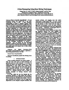
Fig. 1.
TABLE IV E XPERIMENTAL SETUP ( WITHIN THE WEKA ENVIRONMENT ) Algorithm Naive Bayes (NB) Naive Bayes Updateable (NBU) Bayes Net (BN) Logistic (LOG) Simple Logistic (SL) Sequential Minimal Optimization (SMO) Locally Weighted Learning (LWL) Decision Table (DT) One Rule (1R) JRip (JR) Conjuctive Rule (CR) Decision Stump (DS) Logistic Model Trees (LMT)
Several evaluations of the models built using the AG.SOF dataset !"#$ %&'#(() $ * % * #+
Setup Normal distribution for numeric attributes Normal distribution for numeric attributes Local K2 search algorithm, Simple estimator Unlimited iterations, Ridge value in the loglikelihood = 10−8 Cross-validating the number of LogiBoost Iterations: Heuristic stop = 50, Maximum = 500 Weight trimming: beta = 0 Complexity parameter c = 1, Normalized training data, Polynomial kernel, Actual training data used for logistic models Base classifier: Decision Stump, Linear Nearest Neighbour Search (Euclidean Distance), Linear weighting kernel, All neighbours used in the weighting function Cross-validation: leave-one-out, Using IBk (instead of majority class), Maximum non improving tables to consider = 5 Minimun bucket size = 6 Pruning enabled (1 fold used for pruning and 2 for growing the rules), Optimization runs = 2 Reduced-error pruning (1 fold used for pruning and 2 for growing the rules), Non-exclusive expressions for nominal attributes Fast regression heuristic, Cross-validating the number of LogiBoost Iterations, Weight trimming: beta = 0, Minimum number of instances at which a node is considered for splitting = 15
C. Algorithm evaluation on complete datasets – Crossdataset evaluation Having selected the top performing algorithms per station, we proceeded with building the corresponding classifier models using the complete datasets. For each station-algorithm pair, a model was constructed from the complete station’s dataset and was evaluated using 10-fold cross validation. Moreover, due to the nature of the problem at hand, we evaluated each of these models on all stations’ complete datasets, in order to investigate whether, and to what extent, PM10 concentration levels are affected by the stations’ geographic dispersal. Figures 1 and 2 illustrate the evaluation results for models built using the AG.SOF dataset (that records no meteorological data) and the PANORAMA dataset respectively.
Fig. 2. dataset
Several evaluations of the models built using the PANORAMA
D. Discussion of preliminary results All (interpretable) models, reveal the importance of PM10 concentrations during the previous hour, verifying that PM10 forecasting benefits from the use of persistence information [15], [16]. Moreover: • In the AG.SOF station, PM10 concentrations appear to be highly dependent on NO2 , the month, the hour of the day, and the day of the week. This behavior is attributed to the fact that AG.SOF is located in the city center, directly affected by car traffic (a well known source of NO2 ), and from the weekly circle of the city operation. • In the KORD station, PM10 concentrations appear to be highly dependent on SO2 , meteorological conditions (especially wind speed and humidity), the hour of the day, and the day of the week. Moreover, temperature plays an important role in the predictions of exceedances. This finding, in combination with previous ones on source identification of PM10 in Thessaloniki [17] may support the position that combustion sources from industry (a user of fuels with sulphur content) are dominating PM10 production in the west part of the city. The influence of temperature requires further investigation, but it may be related to prevailing weather patters, which still need to be identified in the area. • In the PANORAMA station, PM10 concentrations appear to be highly dependent on NO2 , the month, the day of the week and meteorological conditions. Wind speed and direction play an important role, especially in cases of high or very high PM10 concentrations. • In the SINDOS station, PM10 concentrations appear to be highly dependent on CO, the month, the hour of the day, the day of the week, wind speed and humidity.
Additionally, month, weekday and temperature become decisive factors, when we are facing PM10 exceedances. Thus, again, meteorological patterns and industrial activity seem to be the major parameters influencing this area of the city. J48 is the best performing algorithm, when evaluating the models on the complete dataset they were built from. While this is a very optimistic measure of the resulting models’ accuracy, J48 also performs well, when evaluated using 10-fold cross-validation. However, according to the latter evaluation method, LMT is the top performing algorithm for three out of four stations (AG.SOF:77.6%, KORD:71.9%, PANORAMA:88.76%), with the exception of the SINDOS station, where Decision Table achieves a prediction accuracy of 77.81%. This performance is directly comparable to what has already been reported from previous work for the same pollutant ([15], [16], [18] and references therein). It is worth noting that AG.SOF models present relatively low prediction accuracy (compared to other stations’ models), when evaluated on the actual dataset they were built from. This is an additional indication that meteorological parameters, absent from the AG.SOF dataset, play an important role in the prediction of PM10 concentrations. As far as the other stations’ models are concerned, we should point out that PANORAMA can be predicted with more than modest accuracy (up to 88.76% for model SINDOS-Logistic) by models built using other stations’ datasets. That is interesting when compared to the fact the best performing algorithm for the PANORAMA station (J48) predicts the same dataset with accuracy 91.75%. This may be due to the fact that the PANORAMA dataset presents the lowest percentage of missing and erroneous values and, more importantly, is extremely sparse in terms of PM10 concentrations exceedances (only 1.371% of the records concern PM10 concentration values that are high or very high). Finally, all KORD models perform well when evaluated on the SINDOS dataset (from 72.72% up to 77.4% for model KORD-Decision Table). This finding verifies the geographical interrelation between the two stations as they are both located to the west of the city, and the fact that this part of the city is strongly influenced by industrial and other production activities, that are absent from the rest of the urban web. Moreover, findings indicate meteorological similarities between the two locations that deserve further investigation. IV. C ONCLUSIONS In this paper we have investigated, tested and applied CI methods for studying AQ in the Thessaloniki area, Greece, towards knowledge extraction and parameter forecasting. Both goals were achieved, as the resulting evidence support and expand existing findings concerning the AQ profile of the area, while the achieved prediction accuracy rank among the best described in the literature. On the basis of these findings, further investigation is required concerning the
refinement of the work methodology (by testing, for instance, bootstrapping and genetic algorithms for the selection of proper population for the experiments and parameters of interest). In addition, the need for investigating prevailing weather patterns has emerged, that is expected to help in upgrading the AQ profiling of the area. The same work should be expanded to other pollutants and parameters of interest for the urban environment, including more input especially from the meteorological and emissions domain, if possible. R EFERENCES [1] K. Karatzas, “Internet-based management of environmental simulation tasks,” in Advances in Air Pollution Modelling for Environmental Security, I. Farago, K. Georgiev, and A. Havasi, Eds. Springer, 2005, pp. 253–262. [2] World Health Organization, “Air quality guidelines for particulate matter, ozone, nitrogen dioxide and sulfur dioxide – Global update 2005 – Summary of risk assessment,” [Online], 2005, http://www.who.int/phe/air/aqg2006execsum.pdf. [3] W. Frawley, G. Piatetsky-Shapiro, and C. Matheus, “Knowledge discovery in databases: An overview,” AI Magazine, vol. 13, pp. 57–70, 1992. [4] P.-N. Tan, M. Steinbach, and V. Kumar, Introduction to Data Mining, (First Edition). Boston, MA, USA: Addison-Wesley Longman Publishing Co., Inc., 2005. [5] I. H. Witten and E. Frank, Data Mining: Practical machine learning tools and techniques (2nd Edition). San Francisco: Morgan Kaufmann, 2005. [6] S. K. Murthy, “Automatic construction of decision trees from data: A multi-disciplinary survey,” Data Mining and Knowledge Discovery, vol. 2, no. 4, pp. 345–389, 1998. [7] G. Zhang, “Neural networks for classification: a survey,” IEEE Transactions on Systems, Man and Cybernetics, Part C: Applications and Reviews, vol. 30, no. 4, pp. 451–462, 2000. [8] R. Hanson, J. Stutz, and P. Cheeseman, “Bayesian classification theory,” Tech. Rep., 1991. [9] I. Rish, “An empirical study of the naive bayes classifier,” in IJCAI-01 workshop on Empirical Methods in AI, 2001. [10] D. W. Aha, D. Kibler, and M. K. Albert, “Instance-based learning algorithms,” Machine Learning, vol. 6, no. 1, pp. 37–66, 1991. [11] N. Ye, The Handbook of Data Mining (Volume in the Human Factors and Ergonomics Series). Lea, 2003. [12] B. E. Boser, I. Guyon, and V. Vapnik, “A training algorithm for optimal margin classifiers,” in Computational Learning Theory, 1992, pp. 144– 152. [13] H. G¨usten, G. Heinrich, E. M¨onnich, J. Weppner, T. Cvitas, L. Klainsinc, C. Varotsos, and D. Asimakopoulos, “Thessaloniki ’91 Field measurement campaign-II. Ozone formation in the greater Thessaloniki area,” Atmospheric Environment, vol. 31, no. 8, pp. 1115– 1126, 1997. [14] T. Slini, A. Kaprara, K. Karatzas, and N. Moussiopoulos, “PM10 forecasting for Thessaloniki, Greece,” Environmental Modelling and Software, vol. 21, no. 4, pp. 559–565, 2006. [15] G. Grivas and A. Chaloulakou, “Artificial neural network models for prediction of PM10 hourly concentrations, in the greater area of Athens, Greece,” Atmospheric Environment, vol. 40, no. 7, pp. 1216– 1229, 2006. [16] J. Kukkonen, L. Partanen, A. Karppinen, J. Ruuskanen, H. Junninen, M. Kolehmainen, H. Niska, S. Dorling, T. Chatterton, R. Foxall, and G. Cawley, “Extensive evaluation of neural network models for the prediction of NO2 and PM10 concentrations, compared with a deterministic modelling system and measurements in central Helsinki,” Atmospheric Environment, vol. 37, no. 32, pp. 4539–4550, 2003. [17] E. Manoli, D. Voutsa, and C. Samara, “Chemical characterization and source identification/apportionment of fine and coarse air particles in Thessaloniki, Greece,” Atmospheric Environment, vol. 36, no. 6, pp. 949–961, 2002. [18] G. Corani, “Air quality prediction in Milan: feed-forward neural networks, pruned neural networks and lazy learning,” Ecological Modelling, vol. 185, no. 10, pp. 513–529, 2005.