Mar 11, 1991 - Fitness (percentage correct plus a bonus of five for every feature not used) ...... For example, for the Texas Instruments (TI) 46-word database ...... A.S. Gevins and N.H. Morgan, "Ignorance-based systems," in 1984 IEEE Int.
ESD-TR-90-144
AD-A235 165
_Technical
Report
MAY07 199 1,
*
Using Genetic Algorithms to'Select and Create Features for Pattern Classification
E.I. Chang R.P. Lippmanul
11 March 1991
Lincoln Laboratory MASSACHUSETTS INSTITUTE OF TECHNOLOGY LEXINGTON. MIASSUCHUSETTS
Prepared for lte Defense Advanced Research Projects Agency under Air Force Contract Fl19628-90-C-0002.
Approved for public release; distribution is unlimited.
fDTIC FILE COPY
of
This report
is based on studies performed ait Lincoln Laboratorv, a center for rlesearch op~eratedl by Massachusetts Inlstitute of Jechnolog%. Th'e work was sponsored Ili'the, Defense Advanced Research Projects Agece/DSO under Air Force
Coi'ract. F19628-9t)-C.0002.
The ESD Pbi Affairs Office hia reviewedl tiiis repoirt. aid it isr I-aal tilte National Technical Information Servive. wheit wil be available to t lie g'enera I pubIilic. inc ludlin
This teelinia reor habe reviewed and is approved for pubilication. FORl THlE
ININIE MM
fr Hugh 1,. Souhal U. Co I .UAF Chlief. ESI incol ,aoraov I Project Office
Non-Lincoln Recipients PLEASE DO NOT RETURN Permission is given to destroy this document when it isno longer needed
MASSACHUSETTS INSTITUTE OF TECHNOLOGY LINCOLN LABORATORY
USING GENETIC ALGORITHMS TO SELECT AND CREATE FEATURES
FOR PATTERN CLASSIFICATION
cftw
6
E.I. ClAING
R. P.LIP NNz.a1.o Group 21
r I I
Rk
SDTIC TAB
UI 1= 1-aVd
0
'rc1
)
SAv.ailabtI~ty Ceo .q
TECHNICAL REPORT 892
Di ll
v
11 MARCH 1991
Approved for public release; distribution is unlimited.
LEXINGTON
MASSACHUSETTS
$
07 104
ABSTRACT
Genetic algorithms were used to select and create features and to select reference exemplar patterns for machine vision and speech pattern classification tasks. On a 15-feature machine-vision inspection task, it was found that genetic algorithms performed no better than conventional approaches to feature selection but required much more computation. For a speech recognition task, genetic algorithms required no more computation time than traditional approaches but reduced the number of features required by a factor of five (from 153 to 33 features). On a difficult artificial machine-vision task, genetic algorithms were able to create new features (polynomial functions of the original features) that reduced classification error rates from 19 to almost 0 percent. Neural net and nearest-neighbor classifiers were unable to provide such low error rates using only the original features. Genetic algorithms were also used to reduce the number of reference exemplar patterns and to select the value of k for a k-nearest-neighbor classifier. On a 338 training pattern vowel recognition problem with 10 classes, genetic algorithms simultaneously reduced the number of stored exemplars from 338 to 63 and selected k without significantly decreasing classification accuracy. In all applications, genetic algorithms were easy to apply and found good solutions in many fewer trials than would be required by an exhaustive search. Run times were long but not unreasonable. These resuits suggest that genetic algorithms may soon be practical for pattern classification problems as faster serial and parallel computers are developed.
Ill
TABLE OF CONTENTS Abstract List of Illustrations List of Tables
iii vii xi
1. INTRODUCTION 1.1 1.2 1.3 1.4 1.5
1
Pattern Classification What's a Good Feature? Feature Selection Feature Creation Report Outline
1 2 3 8 12
2. GENETIC ALGORITHMS 2.1 2.2 2.3 2.4
13
Introduction Methods Initial Exploratory Experiments Summary
13 15 18 28
3. NEAREST-NEIGHBOR PATTERN CLASSIFICATION 3.1 Introduction 3.2 The K-Nearest-Neighbor Classifier
29 29
4. FEATURE SELECTION 4.1 4.2 4.3 4.4
35
Introduction Methods Experiments Summary
35 35 36 50
5. FEATURE CREATION 5.1 5.2 5.3 5.4
29
51
Introduction Methods Experiments Summary
51 51 53 54
V
TABLE OF CONTENTS (Continued) 6. INCREASING THE COMPLEXITY OF CREATED FEATURES 6.1 6.2 6.3 6.4
57 57 57 61
Introduction Methods Experiments Summary
7. EXEMPLAR SELECTION 7.1 7.2 7.3 7.4
57
63
Introduction Methods Experiments Summary
63 64 65 74
8. CONCLUSIONS
75
REFERENCES
77
vi
LIST OF ILLUSTRATIONS Figure No.
Page
1
A set of rectangles and triangles that may be inputs to a pattern classifier.
2
2
Decision boundaries of a nearest-neighbor classifier: (a) using both x and y as features and (b) using only the x feature.
5
Classification error rate versus the number of training patterns used to train a nearest-neighbor classifier for the feature set of (x, y) and the feature set of only x.
6
Decision boundaries of a nearest-neighbor classifier: (a) using both x and y features and (b) using the (x/y) feature to classify points on a diagonal line.
9
Classification error rate versus the number of training patterns used to train a nearest-neighbor classifier for the diagonal line problem.
10
A comparison of the distribution of probability of reproduction with selective pressure values of 0.05 and 0.25 and population size of 100.
17
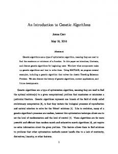
Cumulative distribution of the number of features out of 153 used to calculate Euclidean distances in a k-nearest-neighbor classifier with 90 input and exemplar patterns from the TI 46-word problem.
31
Variation in estimated accuracy (percentage correct) of a nearest-neighbor classifier as more training exemplars are classified using a leave-one-out approach for the parallel vector problem.
34
Fitness (percentage correct plus a bonus of five for every feature not used) versus the number of recombinations for the NMR problem.
37
Genetic algorithm's progress in searching feature subsets for the NMR problem: (a) lowest error rate and (b) minimum number of features.
38
11
Forward and backward sequential search results for the NMR problem.
40
12
The parallel vector problem.
41
13
Forward and backward sequential search results on the training set for the vector problem.
42
Forward and backward sequential search results on the training set for the TI F1 problem.
45
3
4 5 6 7
8
9 10
14
vii
LIST OF ILLUSTRATIONS (Continued) Figure No. 15
16 17
18 19 20 21 22 23
24 25
26
Page Genetic algorithm's progress in searching for feature subsets with high classification accuracy and few features for the TI F1 problem. (a) Classification error rate and (b) number of features used.
46
Forward and backward sequential search results on the training set for the TI F1-F4 problem.
47
Genetic algorithm's progress in searching for feature subsets with high classification accuracy and few features for the TI F1-F4 problem. (a) Classification error rate and (b) number of features used.
49
A block diagram of the feature creation process in which local search is used to eliminate features that are noise.
52
Scatter plot of training patterns for parallel (+) and nonparallel (0) vectors using slope features for the vector problem.
54
Scatter plot of training patterns for parallel (+) and nonparallel (0) vectors using genetic algorithm features for the vector problem.
55
Creating features from original input features to provide better classification accuracy for the parallel vector problem.
56
Creating features out of created features to improve classification accuracy for the parallel vector problem.
58
Distribution of the training patterns belonging to parallel and nonparallel classes when the feature ((dy 2 /dyj)/(dx 2 /dxj)) is used for the parallel vector problem.
59
Creating higher-order polynomial features to reduce classification error rate for the vowel problem.
60
Progress of genetic reduction of exemplars for the vowel problem with k = 1 and only-the-best bonus policy: (a) classification error rate and (b) the number of exemplars used.
66
Progress of genetic reduction of exemplars for the vowel problem with k = 8 and only-the-best bonus policy: (a) classification error rate and (b) the number of exemplars used.
67
viii
LIST OF ILLUSTRATIONS (Continued) Figure No. 27
28
29
30
31 32
Page Progress of genetic reduction of exemplars for the vowel problem with k = 1 and bonus-above-the-threshold policy: (a) classification error rate and (b) the number of exemplars used.
68
Progress of genetic reduction of exemplars for the vowel problem with k = 8 and bonus-above-the-threshold policy: (a) classification error rate and (b) number of exemplars used.
69
Progress of genetic reduction of exemplars for the vowel problem with k = 7 (selected by genetic algorithms) and only-the-best bonus policy: (a) classification error rate and (b) the number of exemplarr' used.
71
Progress of genetic reduction of exemplars for the vowel problem with k = 6 (selected by genetic algorithms) and bonus-above-the-threshold policy: (a) classification error rate and (b) the number of exemplars used.
72
Decision boundaries of a nearest-neighbor classifier for the vowel problem: k = 1 and 338 exemplars.
73
Decision boundaries of a nearest-neighbor classifier for the vowel problem: k = 1 and 43 exemplars selected using genetic algorithms.
74
ix
LIST OF TABLES Table No.
Page
1
Possible Features of a Set of Shapes
3
2
Number of Recombinations Until the Correct Solution Was Found with a Uniform Crossover Operator for the Exponent Problem
19
Number of Recombinations Until the C" rect Solution Was Found with a Two-Points Crossover Operator for the Exponent Problem
20
Number of Recombinations Until the Correct Solution Was Found with a One-Point Crossover Operator for the Exponent Problem
20
Number of Recombinations Until the Correct Solution Was Found with a Unit-Based Crossover Operator for the Exponent Problem
21
The Average and Median Number of Recombinations Until the Correct Solution Was Found Using Different Operators for the Exponent Problem
22
Number of Recombinations Until the Correct Solution Was Found with a Two-Points Crossover Operator for the Exponent Problem Using a Traditional Approach
22
Number of Recombinations Until the Correct Solution Was Found with a Two-Points Crossover Operator for the Linear Problem
24
Number of Recombinations Until the Correct Solution Was Found with a New Two-Points Crossover Operator for the Linear Problem
25
Number of Recombinations Until the Correct Solution Was Found with a One-Point Crossover Operator for the Linear Problem
25
Number of Recombinations Until the Correct Solution Was Found with a Uniform Crossover Operator for the Linear Problem
26
Number of Recombinations Until the Correct Solution Was Found with a Unit-Based Crossover Operator for the Linear Problem
26
The Average and Median Number of Recombinations Until the Correct Solution Was Found Using Different Operators for the Linear Problem
27
The Average and Median Number of Recombinations Until the Correct Solution Was Found Required by Different Operators for the Linear Problem Using Mutative Pressure of 0.25
27
3 4 5 6 7
8 9 10 11 12 13 14
xi
LIST OF TABLES (Continued) Table No. 15
Page Average Number of Recombinations Needed to Find the Best Feature Subset for the Vector Problem
41
16
Features Selected by Genetic Algorithms for the TI Fl Problem
44
17
Comparison Between Sequential Search and Genetic Algorithms for the TI F1 Problem
45
18
Features Selected by Genetic Algorithms for the TI F1-F4 Problem
48
19
Comparison Between Sequential Search and Genetic Algorithms for the TI F1-F4 Problem
49
20
Classification Error Rate for the Vowel Problem as New Features Are Created
61
21
Summary of Using Genetic Algorithms to Select Exemplars
73
xii
1. INTRODUCTION Feature selection and feature creation are two of the most important and difficult tasks in the field of pattern classification. Good features improve the performance of both conventional and neural network pattern classifiers. There is little theory to guide the creation of good features and only some theory in selecting good features. This report explores the application of genetic algorithms to both problems. 1.1
Pattern Classification
The goal of pattern classification is to classify a set of patterns into different classes based on distinguishing characteristics. A pattern may be the outline of a fish, a bark from a dog, or the flag of a nation. Patterns from different classes are made up of features that distinguish these classes. A feature can be any distL.ctive characteristic. For example, the United States flag has the following features: it has 50 stars, 13 alternating stripes, and its colors are red, whi~e, and blue. In designing a pattern classification system, examples of the patterns in each class are typically used to "train" the pattern classifier. These patterns are called the training patterns. Features in patterns can be viewed as defining point: in an input space. Providing more training patterns usually results in a better description of decision regions in the input space, resulting in a more accurate classifier. Decision regions are partitions of the input space into regions where patterns are classified as one particular class. For example, the input space illustrated in the left of Figure 2 has two decision regions. Input patterns that fall into the wnite region are classified as the 0 class, while input patterns that fall into the shaded region are classified as the + class. After a classifier is trained, it must be tested with a different set of patterns called the testing patterns. When a classifier performs well on the testing set, generalization is high. Boundaries between different classes learned from the training patterns are accurate enough so that even a new set of patterns, the testing patterns, c,-" be accurately classified. It is important to have separate sets of training and testing patterns in order to estimate the accuracy of a classifier confidently. The performance of a classifier on training patterns can be overly optimistic because some classifiers, such as nearest-neighbor classifiers, store all training patterns and can classify them perfectly. Accurate estimation of classification performance in real situations requires testing on patterns not used during training. If the total number of patterns is too small to separate the patterns into training and testing sets that adequately characterize the classes, cross validation can be used 16]. In cross validation, a portion of the available patterns is randomly chosen to be used for training, with the remaining patterns used for testing. By averaging the classifier accuracy over different random partitions of training and testing data, a better estimation of the classifier's accuracy can be obtained. With enough training patterns, similar low error rates can be provided using almost any type of neural net or conventional classifier [11]. However, the number of patterns available is often
1
limited by the cost or the difficulty of obtaining more data. It is thus important to select and create good features that provide good performance with a limited number of training patterns. 1.2
What's a Good Feature?
Deriving a good set of features using genetic algorithms is one major goal of this study. An understanding of the relationship between features and classifier accuracy is thus essential. A good feature should make the task of distinguishing between different classes easier without requiring more training patterns. A feature's usefulness depends on the classification task. For example, suppose the triangles and rectangles shown in Figure 1 need to be distinguished. A good feature is the number of sides in the object. Other possible features such as dimension and enclosed area provide no additional information for this task. The number of sides alone is the best feature; all other features are unnecessary and can be considered noise. Conversely, to separate out the objects by their size, the enclosed area of each object is the important feature. A feature is good if it separates classes accurately with as few examples as possible, Table 1 lists some possible object features.
152529-l
T1
T3
R2
/
Figure 1. A set of rectangles and triangles that may be inputs to a pattern classifier.
2
TABLE 1 Possible Features of a Set of Shapes Area
X-Proj
Y-Proj
T-1 R-1
Number of Sides 3 4
0.78 0.54
1.56 1.00
1.00 0.54
R-2 T-2 T-3
4 3 3
0.18 0.32 0.97
0.18 1.00 1.00
1.00 0.64 1.94
Class-ID
If the number of sides is used as one feature, rectangles and triangles (classes R and T) can be specified with only two examples, one from class R and one from class T. The number of sides is thus a very efficient feature to use for classifying objects into rectangles and triangles. On the other hand, if all features are considered, the area of each object is also a reasonable feature; for example, in this given set all objects with area greater than 0.6 are triangles and most objects Nlth area below 0.6 are rectangles. However, because the area is not fundamentally related to the shape of each object, the area feature would not provide reliable classification with new objects. This will only be evident, however, if many training patterns are provided. 1.3
Feature Selection
Having too many input features, also known as the "curse of dimensionality" i1, makes pattern classification problems difficult. As the number of input features increases, the number of training patterns required to maintain good generalization also often increases rapidly and performance with limited training patterns may degrade. When there are many features, more training patterns are needed to fully describe the distribution of the different classes in the multidimensional space spanned by the input features. Because the number of training patterns available is always limited, if there are too many input features, there may not be enough training patterns to design a good pattern classifier. Feature selection (dimensionality reduction) is often required to select the subset of features that best separates classes. Figure 2 demonstrates the effect of feature selection when training data is limited. In this problem, the first class consists of all points with an x coordinate value greater than 3.5. The y coordinate value is random and is not important for classification. A nearest-neighbor classifier was used to demonstrate the concept of decision regions. This classifier stores all reference training patterns (called exemplar patterns) and classifies an unknown input to be in the class of the nearest
3
exemplar pattern (Euclidean distance is used to determine the nearest neighbor). When a nearestneighbor classifier is used with the 16 training patterns shown, the boundary between the two classes, shown on the left side of the figure, is inaccurate because the extra y dimension creates unnecessary sparseness between training patterns. If the y coordinate is eliminated through feature selection, then the boundary between two classes becomes much more accurate as shown in the right side of Figure 2. Figure , plots Lhe error rate of a nearest-neighbor classifier for this problem as the number of trainipg patterns varies from 0 to 500. Each curve is the average of 10 different random trials. Error rates are much lower when only the x feature is used, and an error rate of under 1 percent was achieved with fewer than 50 training patterns. On the other hand, when using both features, the error rate is still above 1 percent even after the number of training patterns is increased to 500. This clearly demonstrates the benefit of selecting good features. Feature selection is difficult because the number of possible combinations of features grows exponentially with the number of original features. For a moderate size problem with 64 features, there are 264 possible subsets of features. Clearly, an exhaustive evaluation of each possible combination is impossible. Frequently, finding a near optimal feature subset is adequate. Many methods exist for finding near optimal solutions. There are two general approaches: heuristically guided search and Monte Carlo approaches. Siedlecki et al. present an overview of these search techniques [18]. Heuristically guided search techniques, such as sequential search, dynamic programming, and branch-and-bound search, utilize heuristics to determine which solutions are to be examined. Monte Carlo approaches, such as simulated annealing and genetic algorithms, rely on selectively added randomness to search for near optimal solutions efficiently. 1.3.1
Traditional Heuristically Guided Search Approaches
Sequential forward search and sequential backward search are the simplest and most widely used of the heuristically guided search techniques [18]. Sequential forward search starts with an empty feature subset, examines each feature's classifier accuracy individually, and puts the best performing feature into the current feature subset. Sequential forward search then looks at all the combinations that include the current feature subset and one of the remaining features and picks the best combination as the new current feature subset. At each cycle the number of features in the feature subset increases by one, while the number of feature pairs examined reduces by one. The process repeats until the feature set grows to the original feature set size or a preset size. A full sequential forward search of a feature set of size N examines roughly (N 2 + N)/2 feature subsets and the number of computations grows as O(N 2). Backward sequential search is similar to forward sequential search except that the search starts with a full feature set. Backward sequential search tries taking out features individually and at each step removes the feature that degrades classifier accuracy the least. At each cycle the number of features in the feature subset is reduced by one, while the number of feature combinations examined is also reduced by one. A full sequential backward search of a feature set of size N also examines roughly (N 2 + N)/2 feature subsets and the number of computations again grows as O(N 2 ). Both sequential forward search and sequential backward search are nonoptimal search procedures in that they are not guaranteed to select the
4
2525292
10
V
3
0 ...+
i
-10
(a) 10
-50 -10
-5
0
5
10
x (b) Figure 2. Decision boundaries of a nearest-neighborclassifier: (a) using both x and y as features and (b) using only the x feature.
152S293
50
40
-,30 LU
20
0
USING TWO INPUT FEATURES (x and y) 0
. 10
U/SING ONE INPUT FEATURE (x)
100
200
300
400
-
500
NUMBER OF TRAINING PATTERNS
Figure 3. Classification error rate versus the number of training patterns used to train a nearest-neighborclassifier for the feature set of (x, y) and the feature set of only x.
best feature subset. They may fail because good individual features do not necessarily combine to form best feature subsets [5]. Sequential search methods can thus miss the best feature subset because they have already deleted or added individual features that were good by themselves but which do not belong in the optimal feature subset. Two feature selection methods, dynamic programming 141 and branch-and-bound search [7], find the optimal feature subset, if certain conditions are met. Dynamic programming is similar to forward sequential search except that it keeps several feature subsets instead of keeping only one. For an original feature set of size N, the dynamic programming approach starts with N feature subsets, each containing one original feature. Individual features are then combined with all feature subsets that do not contain the feature and are assigned to the feature subset that performs the best with the individual feature. The process is repeated until all subsets have grown to the desired feature set size. For a feature set of size N, the dynamic programming approach examines N2 * (N - 1)/2 feature subsets. The number of subsets examined grows as O(N 3 ). The
dynamic programming approach uses more than the O(N2 ) evaluations required by sequential search methods and much less than 0( 2N) evaluations required by exhaustive search. The dynamic programming approach always finds the optimal feature subset when classifier accuracy increases monotonically and when the classifier accuracy of a feature subset is a linear function of classifier accuracies using the individual features within the feature subset. The first
6
requirement, monotonicity in classifier accuracy, states that as the number of features increases, classifier accuracy can only increase or stay the same. As shown in Figure 3, this assumption is not always correct. Depending on the type of the classifier used, extra features may degrade accuracy. The second requirement, separability, states that classifier accuracy on a subset of features and on individual features does not interact. Classifier accuracy of the combined feature set must be a linear function of the individual classifier accuracies. This requiremen, is also often not met. The dynamic programming approach is thus not frequently used [15,18]. Fukunaga's branch-and-bound procedure finds the optimal subset of features when the monotonicity requirement is met [13]. By assuming that as the number of features is reduced, the error rate of a classifier can only increase or stay the same, branches that have very high error rates in a search tree can be disregarded because reducing more features in that subset will not reduce the error rate. The algorithm can thus concentrate on only promising branches and find the optimal feature subset, given sufficient time. In many real-life problems, however, reducing the number of features may actually reduce the classifier's error rate; thus, these problems are not monotonic [5,8]. This restriction and the complexity of the branch-and-bound procedure with high input dimensionality again have limited its application. 1.3.2
Genetic Search
Genetic algorithms have recently been applied with good results to NP complete problems, such as the traveling salesman problem and job scheduling problems [3]. They take advantage of "implicit parallelism" to search efficiently for good solutions 19] and depend on the generationby-generation development of possible solutions, with selection eliminating bad solutions in future generations and allowing good solutions to be replicated and modified. It has also been shown that genetic algorithms are effective in optimizing multimodal and noisy functions 19]. In these applications, each solution manipulated by genetic algorithms represents one possible location of the maxima of a complex function. Solutions specified by bit strings are first randomly generated, then evaluated, and finally manipulated to produce new strings. A suitable function needs to be found for evaluating the fitness of each solution. The selection and search for a better solution is directly affected by the fitness function; thus, the fitness function should be linked tightly to the eventual goal. In pattern classification problems, the usual criterion for success is the percentage of patterns classified correctly. It is thus logical to use the actual classification accuracy as the fitness function of a given subset of features instead of other possible functions, such as the variance of data with respect to tile subset of features. The "training-on-testing-data" problem [6) may appear when the percentage of training patterns classified correctly is used as the fitness function. If the classifier accuracy on the training set is used as the fitness evaluation function, then as better subsets are created at each generation, the feature subsets will gradually be selected based on how they perform according to the testing patterns; in essence, testing patterns have been used as training patterns. There is a danger of finding selections that are good for a particular set of testing patterns yet bad for the general
7
distribution of patterns. This testing on a training data problem can be delayed through using the "leave-one-out" method and cross validation. A different portion of the training patterns is tested at each generation and the feature subsets' performance on this portion of patterns is used for fitness evaluation. However, a separate set of "pure" testing patterns is used to test the performance of feature subsets once feature selection is over. The feature subsets' performance on the pure test patterns is used to verify that feature subsets provide good generalization. Siedlecki has recently successfully applied genetic algorithms to select features for high dimensional problems 120]. However, most of the studies he performed used artificially generated data. The only problem with real data consisted of 150 patterns with an input dimension of 30. Because the number of training patterns was small, apparently the training set consisted of all 150 patterns and no testing set result was reported. As mentioned previously, without checking for the generalization ability of a given set of features, the result obtained on the training set by genetic algorithms may be highly misleading because the genetic feature selection method can overfit the training data. This report compares the genetic search approach with the forward and backward sequential search approaches in efficiency and success of selecting features for several real problems. The sequential approaches were chosen as a basis of comparison because they are the most efficient of traditional approaches and they frequently perform well. Determining the practicality of genetic feature selection is the focus of this research. 1.4
Feature Creation
Feature creation is one of the most important and difficult parts of pattern classification. Created features are normally highly specific to the problem domain. For example, in speech recognition, the distribution of spectral energy may be a useful feature. In machine-vision problems, corners or edges may be useful features. Finding the right features may demand extensive experimentation; yet without good features, it is impossible to provide high classification accuracy. Sometimes higher-order functions of original features can dramatically reduce the number of training patterns needed and improve classification accuracy. One example is a pattern classification problem where all points having equal x and y coordinates form one class and all other points form another class, as illustrated in the left side of Figure 4. The decision boundaries shown in the figure were formed using a nearest-neighbor classifier, as in Figure 2. Using the original features, shown in the left side of Figure 4, provides good generalization only if there are many training patterns that cluster together oit the diagonal line. However, because there are only a limited number of training patterns, it is very likely gaps will occur between points on the diagonal line so that a testing pattern in that gap will be classified incorrectly. Recognizing that higher-order functions of the x and y features are more informative provides better use of the limited training patterns. In this problem, the ratio between the x and y coordinates distinguishes between the classes. Suppose a new system, shown in the right side of Figure 4, is created where only the ratio of the x and y coordinates is used as the feature. In this
8
_______1525294
10
-5
---
-10
x (a)
10
5
V
0
-5
-5
-1-10
-5
0
5
10
X/Y (b)
Figure 4. Decision boundaries of a nearest-neighbor classifier: (a) using both x and y features and (b) using the (x/y) feature to classify points on a diagonal line.
9
case, many fewer training patterns are needed to provide good classification accuracy. All patterns that have a ratio of one belong in the diagonal class and are bounded within the narrow shadowed zone, while all other patterns belong in the nondiagonal class. In this case, it is impossible for a diagonal class pattern to be misclassified using a nearest-neighbor classifier because all diagonal class patterns are on the same point. The chance of nondiagonal patterns being misclassified is greatly reduced as well.
1525295
60
50 C
S40
0.
I-
30
o
USING TWO INPUT FEATURES (xand y)
- 20 USING ONE INPUT FEATURE (x/y)
S. 0
.. 100
... 200
300
400
500
NUMBER OF TRAINING PATTERNS
Figure 5. Classification error rate versus the number of training patterns used to train a nearest-neighborclassifier for the diagonal line problem.
Figure 5 plots the error rate of a nearest-neighbor classifier versus the number of training patterns for this problem. Clearly, by using a good feature (the ratio of x/y), less than 20 training patterns are required to have an error rate of roughly 2 percent. On the other hand, using just the x and y features, even with 500 training patterns, the error rate of the classifier is still well above 2 percent. Many feature creation techniques are available to create new features that are linear combinations of a given set of features. Fisher's linear discriminant approach creates new features in the direction of greatest intraclass variance. Features are thus generated with the hope that they will more clearly separate the classes [6]. Using a Karhunen-L6eve expansion, the original features are
10
transformed into a new set of features with the aim of reducing the correlation between the new features as much as possible. By removing the coirelation between features, it is hoped that the new features with the greatest variance will be the truly useful features. These approaches can reduce the number of input features to a classifier, if only the most useful features are kept. They work well on problems where the patterns are linearly separable in the new feature space. In real problems, it is difficult to know a priori whether a set of patterns is linearly separable in some new feature space. Also, both of these methods examine the statistical properties of the training patterns that may not relate directly to the classifier accuracy. Much research still needs to be done on creating higher-order nonlinear features. For example, given a feature set of x and y, one can readily create a feature z = ax + by with the coefficients a and b calculated using the methods described above. Few methods have been found, however, that effectively create higher-order nonlinear features such as z = x/y or x * y. The number of possible higher-order features grows exponentially with the number of original features. For example, given a problem with three original features x, X2, and X3, the number of unique combinations of these three variables taken two at a time is three. If the number of variables is increased to six, the number of unique combinations increases exponentially to 15. The exponentially growing characteristic of the problem makes an exhaustive search, for even a moderate size problem, computationally infeasible. Only searches of near optimal solutions can be attempted. Tenorio et al. have applied simulated annealing and a tree-based approach to search for the near optimal solutions 121). Other methods such as the Group Method of Data Handling (GMDH) 112 and nonlinear regression can also be used to find higher-order features. These methods rely on local pruning to reduce the number of combinations to be searched. For example, the GMDH approach builds complex functions out of the original features by keeping function sub-blocks that fit the desired output function closely. It can encounter local minima and build very complicated functions when a simpler higher-order function would be better because the local pruning falsely eliminates necessary function sub-blocks. This report explores the use of genetic algorithms to search the space of possible features and find good new high-order features that are nonlinear combinations of original input features. Such higher-order features will improve the efficiency of pattern classification, if the correct problemspecific feature can be found. Higher-order terms can take many forms, and the multiplicative form chosen here is only a small portion of all possible higher-order terms. For example, the multiplicative forms can represent new features such as x 2 * y; however, other possible new features, such as x * ln(y) and (x + y)/(x - y), cannot be found using only a polynomial representation. The type of higher-order terms that provide best performance will be problem dependent. For example, in a time series problem, the Fourier transform of inputs or the cepstrum may be the correct feature to use. In general, any nonlinear function can be chosen by the user to be created and searched using genetic algorithms.
11
1.5
Report Outline
The remainder of this report is organized as follows. Section 2 describes the theory and practice of genetic algorithms. Experimental results of applying genetic algorithms on two simple problems are also presented. Section 3 describes the k-nearest-neighbor classifier and some improvements made to increase efficiency. Section 4 focuses on feature selection. Experimental results on real and artificial problems are presented. Section 5 describes methods and results of applying genetic algorithms to feature creation. Section 6 describes enhancements that increase the complexity of features created. Section 7 presents results of experiments that used genetic algorithms to reduce the number of exemplars needed by k-nearest-neighbor classifiers. Finally, Section 8 provides an overview and discusses future research directions.
12
2. GENETIC ALGORITHMS 2.1
Introduction
Genetic algorithms were first proposed by Holland to optimize functions 12]. Since then, they have been applied to many different types of problems, such as pipeline control, computeraided design, and classifier design 19]. Genetic algorithms emulate Darwin's theory of evolution. A group of possible solutions is judged according to a "fitness" function, which is explicitly related to the objective function to be maximized. Better solutions are chosen and random elements are exchanged between two chosen solutions to generate new possible solutions. The new solutions then undergo mutation, where the bits of the solutions are randomly altered. Afterwards, these new solutions replace members of the old population. If the combination of two partially good solutions yields better solutions, then genetic algorithms will efficiently find near optimal solutions. 2.1.1
Four Stages in Genetic Algorithms
There are four stages in the genetic search process: creation, selection, crossover, and mutation. In the creation stage, a group of possible solutions is randomly generated. In most genetic algorithm applications, each solution is a string of O's and l's. Each string is created by randomly placing O's and l's in the string. After the creation stage, each solution is evaluated and assigned a fitness value. This is followed by a selection stage, where the fitter solutions are given more chance to reproduce. This stage gives the fitter solutions more and more influence over the changes in the population so that eventually fitter solutions dominate. A crossover operation occurs after two fitter solutions (called parent solutions) have been chosen to reproduce. During crossover, portions of the parent solutions are exchanged. This operation is performed in the hope of generating new solutions that will contain the useful parts of both parent solutions and be even better solutions. Crossover is responsible for generating most of the new solutions in genetic search. When all the solutions are similar, the crossover operation loses the ability to generate new solutions since exchanging portions of same solutions generates the same solutions. Mutation is performed on each new solution to prevent the whole population from becoming similar. However, mutation does not generally improve solutions by itself. The combination of both crossover and mutation is required for good performance. 2.1.2
A Simple Example
A simple feature selection problem can be used to demonstrate the basic concepts of genetic algorithms. A string of O's and l's is used to indicate whether a given feature is used. Assume that for a given subset of features, fitness is the percentage-correct score of a nearest-neighbor classifier
13
using this particular subset of features. The goal is to find the optimal feature subset with as few tries as possible. Suppose the ideal feature subset and its fitness value are 10000 90% To find a good feature subset, four procedures of genetic algorithms are performed: creation, selection, crossover, and mutation. In the creation stage, a finite set of possible solutions is randomly generated. For example, in a particular experiment the following initial population may be created: 10110
74%
01101
80%
01011
80%
01010
78%
00011
78%
Initial set of solutions
11110 82% After this initial set has been generated and evaluated as shown above, two solutions are selected to create new strings. This is the process of selection. Just as in nature where the fittest tends to survive, fitter solutions are more likely to be selected. However, weak solutions still have a chance to become parents. Suppose the following two solutions are selected. 01101 01011
80% 80%
Two selected solutions
J
Portions of these solutions are exchanged in order to create new solutions. By performing the crossover operation, new solutions can be created that retain the traits of the parents. A simple type of crossover operation is picking a random point along the solution string and exchanging the solutions' second portion. An example is shown below. 011L11
78%
The new solutions after crossover
0101 82%J The two selected solutions are crossed over to create two new solutions. The lines above and below the two strings are used to distinguish the string portion of one selected solution from that of the other.
14
After crossover, the newly created solutions are randomly mutated. This mutation is necessary because sometimes all the solutions in the population are very similar. Even exchanging portions of different solutions creates no new solutions. With a small amount of mutation, however, new solutions are created to introduce more diversity into the population. In the current example, suppose the first new string is randomly changed at one position identified by the - sign. 01611
80%
} Mutated solution
In this case the mutation was fortuitous because it improved the modified solution's fitness value from 78 to 80 percent. This improvement does not always happen and is not the main purpose of performing mutation. Mutation's chief contribution is preventing premature convergence of the whole population of solutions, i.e., the whole population having similar solutions. Without mutation, once premature convergence occurs, genetic search stops. This process of selection, crossover, and mutation would normally be continued through many generations in this problem until an acceptable solution was found. As can be seen by this example, many new strings may need to be created because there is no guarantee that crossover and mutation will always lead to fitter strings. 2.2
Methods 2.2.1
Introduction
There are many varieties of genetic algorithms. In the original simple models, all members of a population completely reproduce at every generation. In more complicated models, "niches" are formed in the population and "migration" is allowed within niches 19]. This study used an incremental approach that has been used successfully in other areas and was found to work well in initial exploratory experiments. 2.2.2
Static Population Model
The relatively new incremental static population model proposed by Whitley [23] was used in all experiments. In the regular genetic algorithm model, the whole population undergoes selection and reproduction, with a large portion of the strings replaced by new strings. It is thus possible for good strings to be deleted from the population. In the static population model, the population is ranked according to fitness. At each recombination cycle, two strings are picked as parents according to their fitness values and two new strings are produced. These two new strings replace the lowest-ranked strings in the original population. This model automatically protects the better strings in the population, so that the best string found so far always stays in the population. Also, because changes in the population are incremental, a large portion of the population is never replaced by worse strings (this can conceivably happen in the regular generation model).
15
2.2.3
Rank-Based Selection
Genetic algorithms rely on likelihood of that better strings to reproduce to increase search efficiency. In the experiments performed, a rank-based selection approach was used to select parents. In the typical genetic algorithm model, the probability of a string i becoming the next parent, p(i), is calculated as follows: p(i) - c * f(i)/f(avg). Here. f(i) is the fitness of the string i, f(avg) is the average fitness of the whole population, and c is a constant selected by the user. If the fitness of string i is 10 times greater than the average fitness, it would be 10 times more likely than an average string to reproduce. This selection scheme can fail due to the large differences between fitness values. For example, if the average fitness value is 10, yet two strings have the fitness values of 90, clearly these two strings will be selected most of the time. When both of the parents are the same, the crossover operator has no effect and gradually tile whole population becomes duplicates of the fittest strings. No new strings are created and the search halts. This phenomenon defeats the purpose of a genetic algorithm's search and is similar to the phenomenon of "inbreeding" noted by biologists. To prevent superbly fit individuals from dominating a population, various scaling schemes have been proposed. For example, the value of c can be periodically adjusted when the probability of reproduction is assigned. In the beginning of the search, when a few strings are more likely to have a high fitness value relative to the average fitness value, the constant c is adjusted lower. At the latter part of the search, when the difference between the best string's fitness value and the average string's fitness value is smaller, the constant c is increased to ensure that the best strings do get more chances to reproduce. There are many problems in using the fitness values themselves to compute the probability of reproduction directly. By using the rank-based selection scheme, all these problems can be avoided 123]. In a rank-based system, all the strings within the population are ranked according to their fitness value. A variable called selective pressure is used to determine how much the top strings are favored. The probability to reproduce is computed with the following iterative equations: p(l) = 1.0 * selective pressure, i
p(i + 1) = (1.0 - Ep(j)) * selective pressure, j=l
where string 1 is the most fit solution and probabilities are assigned to the fittest solution first. This scheme gives exponentially more reproduction opportunity to fitter strings. Also, because only the relative rank of the strings affects the probability of reproduction, changes in the distribution of fitness values have no effect as genetic search progresses. An additional benefit is that bias toward good strings can be controlled by varying the selective pressure variable. For example, Figure 6
16
shows that the distribution of the chance to reproduce changes visibly when the selective pressure is changed from 0.05 to 0.25.
0.3
1
1
1
1
1
1
1
1525n-6
1
1
>- 0.2 .1I
0.
0.1
SELECTIVE PRESSURE = 0.25-
-
SSELECTIVE PRESSURE 0 0
I . t_ 10 20 30
40
50 60 70
= 0.05
80 90 100
RANK IN THE POPULATION
Figure 6. A comparison of the distribution of probability of reproduction with selective pressure values of 0.05 and 0.25 and population size of 100.
2.2.4
Crossover Operators
Many different techniques can be used to create new strings by crossing over old strings. A uniform crossover operator, one-point crossover operator, two-points crossover operator, or unit-based operator can be used. With the uniform operator, random bits of each string are independpntly chosen to be crossed over. With the one-point crossover operator, a random point is chosen in the string and the substring starting from the chosen point until the end of the string is exchanged. With the two-points crossover operator, two random points are picked within the strings and the substring between the two chosen points is exchanged. With the unit-based crossover operator, substrings are exchanged in unit lengths that relote to the encoding of the string. For example, suppose a string 12 bits long represents four numbers, with three bits representing each number. Using the unit-based crossover operator, the substring exchanged between strings can only start at 1, 4, 7, 10, and end at 3, 6, 9, 12. Because the bit string encoding is ultimately translated back to integer values, it may be more efficient to exchange substrings between strigs only in the unit of
17
integers. The unit-based operator keeps each integer represented in the bit string intact even after crossover. After some initial comparison of crossover operators in solving simple problems, the two-points crossover operator and the uniform crossover operator appeared most consistent in providing good results. Both were used as crossover operators in the rest of the experiments. 2.2.5
Mutation Operator
Mutation increases the diversity of strings in a population. In the standard genetic algorithm, the mutation probability is usually set in the range of 0.01 to 0.001. By using low mutation values, the genetic search depends on the crossover operation to create new strings that are yet unexplored. An adaptive mutation rate approach suggested by Whitley [24] was used in all experiments. This approach uses the hamming distance between the two parents as a measure of their similarity. If the hamming distance is large, then the mutation rate is reduced. If the hamming distance is small, then the mutation rate is increased. More specifically, the mutation rate is calculated with the following equations: mutative pressure p(mutation)
=
if hamming distance > I
hammig dstance
mutative pressure if hamming distance = 0 Because the crossover operation depends on exchanging portions of the parent strings that are different, the adaptive mutation rate ensures that when parents are very similar, different strings are still produced. When the crossover operator becomes ineffective as a mean of generating new strings, the mutation operator becomes more influential in generating new strings. 2.3
Initial Exploratory Experiments 2.3.1
The Exponent Guessing Problem
Problem Description. The effectiveness of genetic algorithms in searching for functions was tested using two artificial problems. The first problem was an exponent guessing problem that evaluated the ability of genetic algorithms to select parameters of a function. A four-variable function t(a, b, c, d) = ai. bj* * * dl was used as the target function. Each individual string within the population contained 12 bits, with 3 bits identifying the exponent of each variable, ranging from -3 to 3 (with 0 being represented twice). The difference 6 between the desired function to and the function guessed by a genetic algorithm was summed over the integer range (0 < a < 5, 0 < b < 5, 0 < c < 5,0 < d < 5). The ratio 1/(E 6 + 0.001) was used as the fitness function to evaluate the fitness of each individual string. The small value 0.001 was added to the overall sum to avoid dividing by zero when the correct function was found.
18
This experiment was performed to see whether genetic algorithms are able to find the correct function that maximizes fitness. When creating features, as described in Section 5, different highorder functions of basic features are searched; it is thus important to test the genetic algorithm's ability to create functions. There had been no previous results on using genetic algorithms to create functions, and it was uncertain whether genetic algorithms would work well on this problem. Results. Sets of experiments using different crossover operators, mutative pressure, and selective pressure were run. The results are shown in Tables 2 to 5. Ten independent trials were run for each combination of selective pressure, mutative pressure, and crossover operator. The numbers shown in the tables are the average number of recombinations over the 10 trials required before the perfect answer was found. Each trial was stopped once the number of recombinations reached 1001. The original population size was 100; therefore, 100 evaluations for the original population plus the number of recombinations equals the total number of evaluations used before the correct function was found.
TABLE 2 Number of Recombinations Until the Correct Solution Was Found with a Uniform Crossover Operator for the Exponent Problem 0.0
0.25
0.5
0.75
1.0
0.00 0.05 0.10 0.15
387 387 713 705
247 109 70 282
452 265 219 137
515 320 423 300
862 244 449 169
0.20
804
143
293
374
305
0.25
902
212
172
225
373
Mutative Pressure
Selective Pressure
The bit strings in this problem were 12 bits long. One of the exponents to be guessed was zero, which could be represented with two distinct combinations (000 and 100), so the total number of distinct strings was 211, or 2,048. An average of 1,024 evaluations would thus be needed in a random search procedure. Tables 2 to 5 show that as long as a selective pressure of 0.0 or a mutative pressure of 0.0 was not used, genetic algorithms always required fewer evaluations than the random search procedure. Furthermore, except when mutative pressure or selective pressure equaled 0.0, there was no general trend in the number of recombinations required for different selective and
19
TABLE 3 Number of Recombinations Until the Correct Solution Was Found with a Two-Points Crossover Operator for the Exponent Problem Mutative Pressure
Selective Pressure
0.0
0.25
0.5
0.75
1.0
0.00 0.05
447 902
432 374
648 252
664 281
442 374
/0.10 0.15
809 901 901 1001
159 160 216 246
334 134 348 589
293 397 334 389
322 446 310 285
0.20 0.25
TABLE 4 Number of Recombinations Until the Correct Solution Was Found with a One-Point Crossover Operator for the Exponent Problem Mutative Pressure
Selective Pressure
0.0
0.25
0.5
0.75
1.0
0.00
406
451
373
507
453
0.05
708
266
327
374
385
0.10 0.15 0.20
906 710 1001
174 297 106
324 177 248
250 280 540
180 342 377
0.25
901
378
179
358
474
20
TABLE 5 Number of Recombinations Until the Correct Solution Was Found with a Unit-Based Crossover Operator for the Exponent Problem Mutative Pressure
Selective Pressure
0.0
0.25
0.5
0.75
1.0
0.00
504
459
436
509
603
0.05 0.10 0.15
721 704 1001
312 165 226
125 316 195
319 342 244
371 373 462
0.20 0.25
902 701
236 278
297 266
412 358
333 343
mutative pressure values. Genetic algorithm search appeared to be robust to the values chosen and worked better than a random search for a wide range of values. Table 6 lists the average and the median number of recombinations for a mutative pressure range of 0.25 to 0.75 and a selective pressure range of 0.05 to 0.25 required by each crossover operator. The uniform operator required fewer recombinations than the two-points crossover operator; however, the difference was small. No crossover operator performed an order of magnitude better than other operators. All operators required more than a factor-of-three less evaluations than would be required by an average random search. Another set of experiments was performed using the traditional generation model on the same exponent guessing problem. Three sets of experiments, each consisting of 10 independent trials, were performed. The population size was also 100, the probability of reproduction was 60 percent, and the mutation rates were 0.001, 0.01, and 0.10, respectively. In any given generation, 60 percent of the strings were likely to be reproduced. The expected number of recombinations per generation was thus 60. The average number of recombinations required for the three sets of experiments is listed in Table 7. The generation approach was not as efficient as the static population model approach. For example, the average number of recombinations with the two-points crossover operator and the static population model was 300, yet all three trials of the generational model required more than 500 recombinations. This difference in efficiency is due to the many new strings that are generated in each generation, so a good string can reproduce many times in one generation. This excessive reproduction results in homogeneity in the population and premature convergence. In
21
TABLE 6 The Average and Median Number of Recombinations Until the Correct Solution Was Found Using Different Operators for the Exponent Problem Operator
Average
Median
Uniform
236.3
219
Two-Points
3004
281
One-Point Unit-Based
285.2 272.7
266 266
TABLE 7 Number of Recombinations Until the Correct Solution Was Found with a Two-Points Crossover Operator for the Exponent Problem Using a Traditional Approach Mutative Pressure
Average Number of Recombinations
Standard Deviation
0.001
540
180
0.01 0.10
1020 840
300 180
22
this experiment, the best string was always kept in the population, further increasing the chance of premature convergence. 2.3.2
The Linear Combination, Guessing Problem
Problem Description. This problem tested the ability of genetic algorithms to find a combination of functions simultaneously. In feature creation, a set of features may need to be found at the same time in order for the classifier to benefit from them. To test the effectiveness of genetic algorithms in guessing a set of functions, the second problem was designed to be a search of a linear combination of functions. In this problem, genetic algorithms were used to find the variables and exponents of the function to = x, 31 + x * y + x' *3 +1 . The x and y variables could be any of the four variables a, b, c, and d. The exponent of each variable was either 1 or -1. Two bits were used to identify the variable and one bit was used to indicate the exponent of the variable. Each of the product terms in the equation thus required six bits. The whole equation required a total of 18 bits. The actual function to be guessed was to = a * b + a * c + bid. Again, the fitness function used was 1/(E 6 + 0.001), the inverse of the difference 6 between the function guessed by genetic algorithms and the actual function over the range of 0 to 5 for each variable. To prevent dividing by zero when the perfect solution was found, a very small value ( 0.001) was again added to the sum of differences. The fitness value of the perfect string is thus 1,000. Results. Experiments were again performed using different'selective pressure, mutative pressure, and crossover operators. The average numbers of recombinations required before the correct solution was found are listed in Tables 8 .. 12. The total number of evaluations used was the initial population size (100) plus the number of recombinations. This linear combination problem had an encoding length of 18 bits. However, there are some redundant solutions; for example, the term a * b is the same as the term b * a. The actual number of distinct solution is (25) 3 , or 32,768. Out of the 32,768 solutions, there are 3! correct solutions because the three terms in the target equation can be rearranged. The probability of successfully guessing the correct solution in a random trial is then 6/32,768. The expected number of trials required in a random search procedure is 1/2 * 6/32,768 = 2,730. Table 8 lists the number of recombinations required when the original two-points crossover operator is used. As long as a mutative pressure of 0.0 or 1.0 and a selective pressure of 0.0 are not used, the average number of recombinations is 446. After adding 100, the number of evaluations required for the starting population, the total of 556 is still much less than 2,730. Genetic algorithms performed better than random search for all four types of crossover operators. The operator tested in Table 8 first uniformly picked a point, then picked a second point uniformly between the first point and the end of the string. The portion between the first point and the second point was exchanged. This operator differed from an alternative form of two-points crossover operator, where both points were picked uniformly along the length of the string, with the smaller number becoming the starting point.
23
The experiment with the second type of two-points crossover operator is shown in Table 9. There is no significant difference between Tables 8 and 9. There was also no clear advantage in using the one-point crossover operator (Table 10), the uniform operator (Table 11), or the unitbased operator (Table 12). An operator might have been better at a particular setting of selective and mutative pressures, but no operator was consistently better than all the others.
TABLE 8 Number of Recombinations Until the Correct Solution Was Found with a Two-Points Crossover Operator for the Linear Problem Mutative Pressure
Selective Pressure
0.0
0.25
0.5
0.75
1.0
0.00 0.05
1106 2413
478 449
285 317
735 336
961 599
0.10 0.15 0.20 0.25
2711 2704 2405 3001
313 355 686 309
337 544 561 558
634 493 419 382
400 945 965 866
Table 13 shows the average and the median number of recombinations for the mutative pressure range of 0.25 to 0.75 and selective pressure range of 0.05 to 0.25. These ranges were chosen to remove the results of using extreme mutative and selective pressure values. Within the ranges, the two-points crossover operator performed the best and the uniform crossover operator performed the worst. The results differ with the results shown in Table 6, when the uniform operator performed the best and the two-points crossover operator performed the worst. Table 14 shows the average and the median number of recombinations when the mutative pressure is 0.25 and the selective pressure range remains at 0.05 to 0.25. In this table, the new two-points crossover operator turned out to be the best in terms of average, while the uniform crossover operator was the best in terms of median. Depending on the selective and mutative pressure range, one operator may be superior to another. However, no result convincingly shows one crossover operator to be better than other operators. In this report, the two-points crossover operator was used for feature selection and feature creation problems for consistency. On problems with longer strings such as the experiments described in Section 7, the uniform crossover operator was used. These choices were made based
24
TABLE 9 Number of Recombinations Until the Correct Solution Was Found with a New Two-Points Crossover Operator for the Linear Problem Mutative Pressure
Selective Pressure
0.0
0.25
0.5
0.75
1.0
0.00 0.05 0.10
680 1558 2403
698 392 614
562 415 506
804 585 511
948 405 705
0.15 0.20
2703 3001
0.25
2402
303 369 583
453 572 517
691 640 392
520 510 615
TABLE 10 Number of Recombinations Until the Correct Solution Was Found with a One-Point Crossover Operator 'cr the Linear Problem Mutative Pressure
Selective Pressure
0.00 0.05 0.10 0.15 0.20 0.25
25
0.0
0.25
0.5
0.75
1.0
1088 1855 2125 3001 2702 3001
564 282 341 480 271 496
671 306 423 258 334 797
522 808 745 582 763 650
1095 867 552 523 628 668
TABLE 11 Number of Recombinations Until the Correct Solution Was Found with a Uniform Crossover Operator for the Linear Problem Mutative Pressure
Selective Pressure
0.00 0.05 0.10 0.15 0.20 0.25
0.0
0.25
f).5
0.75
1.0
846 760 2130 2707 2703 2402
488 271 298 567 399 291
721 552 533 346 491 965
950 762 703 876 569 1142
801 1044 1480 1068 1031 1083
TABLE 12 Number of Recombinations Until the Correct Solution Was Found with a Unit-Based Crossover Operator for the Linear Problem Mutative Pressure
Selective Pressure
0.0
0.25
0.5
0.75
1.0
0.00 0.05 0.10
864 3001 2117
458 416 353
462 364 492
385 505 465
907 528 699
0.15 0.20
2406 2406
244 371
453 507
438 546
765 949
0.25
2403
328
815
990
902
26
TABLE 13 The Average and Median Number of Recombinations Until the Correct Solution Was Found Using Different Operators for the Linear Problem Operator
Average
Median
Uniform Two-Points New Two-Points One-Point
584.3 446.2 502.9 502.4
533 382 506 480
Unit-Based
556.5
438
TABLE 14 The Average and Median Number of Recombinations Until the Correct Solution Was Found Required by Different Cpzrators for the Linear Problem Using Mutative Pressure of 0.25 Operator
Average
Median
Uniform Two-Points New Two-Points
365.2 422.4 252.2
298 355 392
One-Point Unit-Based
374.0 342.4
341 353
27
on the experience that no one operator performed an order-of-magnitude better than the others. Completely analyzing the performance of all crossover operators for the type of problems studied in this report would have taken too long, so no further studies on the effect of using different operators were pursued. 2.4
Summary
This section describes the genetic algorithm approach selected for this study and the effect of using different mutative pressures, selective pressures, and crossover operators. Although small aifferences exist between the performances of different crossover operators, they are not large enough to favor selecting one operator over another. No specific set of selective and mutative pressure values was good for all experiments, but mutative pressures of 0.25 and 0.5 and selective pressures from 0.05 to 0.25 appeared to work well in all problems. The standard two-points crossover operator and the uniform crossover operator were used for further experiments with parameters chosen from this range. With choices from these ranges, genetic algorithms on average found the correct function for two artificial function selection problems in one-fifth to one-half as many trials as would be required on average by a random search procedure.
28
3. NEAREST-NEIGHBOR PATTERN CLASSIFICATION 3.1
Introduction
Genetic algorithms for feature selection require a fitness function to estimate the usefulness of a set of features. The most direct way of determining the usefulness of a set of features is to actually use the features with a pattern classifier. In this report, the percentage correct from a k-nearest-neighbor classifier was used as the evaluation function. This section briefly describes the k-nearest-neighbor classifier and enhancements that reduce computation requirements. 3.2
The K-Nearest-Neighbor Classifier 3.2.1
History
The k-nearest-neighbor classifier has been used as a reference classifier by many researchers in the neural networks field [11. It has the advantage of not requiring a training phase and providing good accuracy when there are sufficient training patterns that are representative of the overall pattern distribution. It has been proven that the error of the nearest-neighbor classifier is bounded by twice the Bayes error when the number of training patterns is large (6). Previous work has also demonstrated that the relative performance of a feature set found using a k-nearest-neighbor classifier is closely related to the relative performance of other classifiers 18,11]. 3.2.2
Descripiion
A k-nearest-neighbor classifier compares the Euclidean distance between a pattern to be classified with all stored training exemplar patterns. The unknown pattern is assigned the class label that occurs most frequently among the k-nearest-neighbor training patterns. The only training required is storing all the training patterns in memory. The procedures of training and using a k-nearest-neighbor classifier are: * Training 1. Store all training patterns in memory along with their class labels. * Classification 1. Present an unknown pattern to be classified. 2. Find the k-nearest neighbors of an unknown pattern by calculating the Euclidean distance between the unknown pattern and the stored exemplars. 3. Assign to the unknown pattern the class label that occurs most frequently among the k-nearest neighbors. In case of a tie between classes, break the tie randomly.
29
Because genetic algorithms rely on trying many possible solutions, the k-nearest-neighbor classifier is attractive because it requires little training. A different type of pattern classifier, the radial basis function classifier 112,17], was also used as a pattern classifier in initial experiments. However, using the radial basis function classifier took considerably longer and did not always provide large improvements in accuracy. Thus, the k-nearest-neighbor classifier was used in all experiments. Because computation requirements increase as k increases, k was set to 1 for all experiments except when genetic algorithms were used to choose exemplars, as described in Section 7. 3.2.3
Efficiency Improvements
Although the k-nearest-neighbor classifier requires little training, the amount of time required to classify input patterns is considerable, especially when there are many example patterns and the input data has high dimensionality. When using "leave-one-out" cross validation to estimate error rates (6], the Euclidean distance between every exemplar pattern taken one at a time and other exemplar patterns must be calculated. Computation thus increases as O(N 2 ) where N is the number of exemplar patterns. Two improvements were made to the basic nearest-neighbor classifier to reduce computation requirements. Comparison with the Shortest Squared Distance. Any method that can cut down the number of operations performed in distance calculations will reduce the execution time of a k-nearestneighbor classifier. One such method that does not require much memory or time is to terminate distance calculation on an exemplar if it cannot be closer than the kth-nearest neighbor found so far. An algorithmic description of the method follows. In calculating the distance to each exemplar pattern with d as the input dimension and Sum as the total squared distance to the exemplar: 1. Sum = 0,i = 1 . 2. Calculate d?, the squared difference between feature i of the exemplar pattern and that of the input pattern. 3. Sum = Sum + d? . 4. If Sum > minimum squared distance to the kth-nearest neighbor found so far, then this exemplar is done. 5. Else, i= i + 1. 6. If i < d, then go to step 2. 7. Else, this exemplar is done. This distance calculation proceeds by iteratively summing the squared distances between features in the input and the exemplar patterns, one feature at a time.
30
When the sum is greater than the squared distance to the kth-nearest neighbor found so far, then clearly the current exemplar cannot be one of the k-nearest neighbors and the extra computation for the remaining features can be eliminated. This method requires an extra comparison at each dimension. For low dimension problems on a Sun 3/110 workstation with a floating-point accelerator, the time used for performing the comparison may be longer than the amount of time saved by avoiding more calculations in further dimensions. However, for problems with a large number of features, as the sum of squared differences is progressively increased, it becomes more and more likely will be greater than the kth-nearest squared distance found so far. The chance of avoiding many calculations is high and the likely saving in time is large.
152529 I
100 90
(50 80
zw
M 70
o W 60 0
LL
50
X 40
o 30 CL - 20 10
I
0o 0
20
40
60
80
100
120
I 140 160
N= NUMBER OF FEATURES USED Figure 7. Cumulative distribution of the number of features out of 153 used to calculate Euclidean distances in a k-nearest-neighborclassifier with 90 input and exemplar patterns from the TI 46-word problem.
For example, for the Texas Instruments (TI) 46-word database problem described in the next section, there are 153 input features. If a k-nearest-neighbor classifier with k = 1 is used with 90 training patterns, each distance calculation requires 305 additions plus subtractions and 153 multiplications per input pattern. With the modification, the cumulative distribution of the number of features used to calculate distances is shown in Figure 7. As can be seen, more than
31
50 percent of the distance calculations were completed before calculation proceeded to 80 features. The average time used by the modified version of the k-nearest-neighbor classifier in one experiment was 1.81 sec. This is 44 percent less than the 3.21 sec used by the unmodified version. All times were measured on a Sun 3/110 workstation with a floating-point accelerator in an experiment with 90 input patterns. Conditionally TerminatingEvaluation. While the above modification to the k-nearest-neighbor classifier does not introduce new errors, another modification (conditionally terminating evaluations) can statistically create new errors. However, the amount of time saved makes it worthwhile to accept the small risk of not accurately estimating the classifier accuracy. Before introducing the approach, the reason for its use needs to be explained. In the experiments performed in this report, there were two classifier accuracies: the accuracy of the training set and the accuracy of the testing set. The accuracy of the training set was the fitness function value used in the genetic search, while the accuracy of the testing set was not used in the genetic search. Separating patterns into training and testing sets allows the generalization ability of the genetic search's solution to be checked. However, the k-nearest-neighbor classifier with k = 1 has an accuracy of 100 percent on the training patterns because the nearest neighbor of a pattern is itself. To avoid this problem, the leave-one-out approach was used 16]. In this approach, every pattern in the training set is classified using the training set with itself removed. The overall accuracy of the training set is the number of correct classifications divided by the total number of patterns in the training set. In many problems the size of the training set is large; thus, calculating the training set accuracy using the leave-one-out approach takes a long time. It requires classifying each exemplar pattern using N(N - 1) Euclidean distance computations. Conditionally terminating evaluation is based on the idea that the eventual classification accuracy of the training set can be adequately estimated using only a small portion of all the training patterns. At intervals of 50 training patterns, the program estimates the error rate and calculates the expected deviation from the true error rate with the following equation:
S
(1 -p)*p
In this equation p is the estimate of probability of correct classification obtained so far and n is tile number of samples tested so far. The value p is calculated with the following equation:
P=
Number of training patterns correctly classified so far Number of training patterns classified so far
32
Every 50 patterns, the sum of p and 2 * a (two times the standard deviation) is compared with the best performance obtained so far. If the sum of p and 2 * a is less than the best accuracy so far, then testing is stopped and the program accepts p * 100 as the percentage correct. This procedure works because the percentage correct usually stabilizes quickly as one goes through the patterns in the training set. Thus, the final percentage correct can be estimated from the percentage correct calculated with a smaller sample set size. For example, Figure 8 shows that as the number of samples evaluated increases for the vector problem discussed in Section 4, the percentage correct gradually stabilizes and the final percentage correct is not far from the percentage correct calculated at n = 100. When n = 50, the estimated percentage correct plus two standard deviations is greater than the best percentage correct found so far, so the calculation continues. At n = 100, the estimated percentage correct plus two standard deviations is below the best percentage correct found so far, so the program would stop and accept the current estimated percentage correct as the final value. Because the percentage correct is far from the best percentage correct found so far, slight inaccuracy in classifier accuracy does not affect the genetic search. Assuming that the deviation of p from the true percentage correct is a Gaussian random value with a mean of 0, there is only a 2.3 percent chance that the true percentage is greater than p + 2 * a. There is thus only a one-in-forty chance that the accepted percentage correct would be lower than the percentage correct obtained when all patterns in the training set are classified. When genetic algorithms are used for feature creation, the best feature subsets are frequently outstanding compared with the average feature. The feature subsets that have a low percentage correct compared with the best feature subset encountered so far do not require accurate estimations of their accuracy. By using this approach and the above rule, the amount of computation required by the parallel vector problem, described in the next section, was reduced by a factor of six. Because genetic algorithms took days to run, a reduction from six days to one day was significant. Accepting a 2.3 percent probability of a large estimation error resulted in much shorter computation time and made this research possible.
33
I8
100
"°
go
IS25I
BEST PERCENTAGE CORRECT SO FAR-
80 70 PERCENTAGE CORRECT + 2 STANDARD DEVIATIONS
Up 60
w50
PERCENTAGE CORRECT
M 40 0 M 30 w 2010 0
50 100 150 200 250 300 NUMBER OF TRAINING POINTS CLASSIFIED
Figure 8. Variation in estimated accuracy (percentagecorrect) of a nearest-neighborclassifier as more training exemplars are classified using a leave-one-out approach for the parallel vector problem.
34
4. FEATURE SELECTION 4.1
Introduction
Feature selection involves selecting that subset of features from a large initial set that provides best classification performance. As mentioned previously, for a problem with high dimensionality, conducting a full search through all the possible feature subsets is infeasible. This report focuses on genetic algorithms and uses forward and backward sequential search as a reference for comparisons. 4.2
Methods 4.2.1
Representation and Evaluation
Every feature set or possible solution is represented by a bit string with d bits, where d is the maximum input dimension. Each bit of a solution represents a feature. If the bit is 1, then the feature is used; otherwise, the feature is not used. Many different evaluation functions have been suggested to differentiate between good and bad feature subsets. Most are statistical and indirect and make strong assumptions on data distributions 16,15]. The accuracy of a nearest-neighbor classifier was used as the evaluation function in this study. The nearest-neighbor classifier has the advantages of requiring no training time and providing results directly related tp performance. 4.2.2
Feature Reduction
The goals of feature reduction are twofold: feature reduction and classifier performance improvement. These two goals may conflict with each other, as in cases where the full feature subset is actually the feature set to use if best classifier performance is required. In some cases, however, reducing the number of features is more important than finding the best performing feature set possible. For example, the storage of the extra features may be very expensive and the collection of additional features may be time-consuming. By reducing the number of features required, one call directly reduce memory requirements and the expense of collecting training data. If classifier performance is used as the fitness function, genetic search will find a set of features with the best classifier performance and not necessarily reduce the number of features used. There must be an incentive for feature reduction to take place. In the experiments performed in this study, feature reduction was an option that could either be used or not used. When the feature reduction option was used, an incentive in the form of a "bonus" was given to good strings that did not use many features. The bonus was a constant multiplied by the number of features not used, and it was added to the classifier performance to derive the .atness value of the string. Two different methods of giving the bonus were tried. In one policy called "only-the-best," only the string that performed better or equal to the best string so far would receive a bonus. This policy had the effect of ensuring that classification accuracy was not compromised for the sake of
35
reducing the number of features used. If the full feature subset turned out to be the best set, then it would still have a higher fitness value than other subsets that used fewer features but had a lower classification accuracy. Another policy of giving the bonus was called "bonus-above-thc chreshold." With this policy, the user specified an acceptable percent-correct threshold. All strings equaling or surpassing the standard would get a bonus proportional to the number of features they did not use. By using this policy, the user could specify that feature reduction was the more important goal once a certain minimum performance standard was achieved. With this policy, it was possible for a string with a lower classification accuracy to have higher fitness value because it used fewer features. This policy is useful if an acceptable threshold can be found. It may be difficult to use if selecting a minimum performance threshold is a problem. 4.2.3
Reshuffling
With the only-the-best policy, the fitness function is time-varying because it depends on the best performance measured so far. This factor causes strings evaluated earlier in the population to have an advantage over latter strings. Because the first string to be evaluated is compared with a classification accuracy of zero, it will definitely receive a bonus. It will be more difficult for latter strings to receive the bonus. In some cases, two identical strings, one evaluated at the beginning and one evaluated near the end, will have different fitness values. To avoid biasing the population by favoring the strings evaluated earlier, a procedure called "reshuffling" took place periodically. When reshuffling was performed, the classification accuracy of all the strings was compared with the best classification accuracy obtained thus far. Periodic reshuffling was essential to rank all solutions using the same fitness function. 4.3
Experiments 4.3.1
The NMR Problem
Problem Description. The first data used for feature selection, a General Electric Corporate Research and Development database, contained 387 patterns, each with 15 featureb, for four different classes of patterns. The 15 features were derived from the intensity histogram of nuclear magnetic resonance (NMR) test images that were generated for calibration and test purposes using a standard glass sphere. Within the data were 27 normal patterns, 72 chopped phase shift patterns, 144 spike patterns, and 144 phase shift patterns. The latter three classes were defective images that would be obtained from hardware faults in the image processor. With this database, the goal was to distinguish between the patterns of the normal case and that of the three defective cases. Results. The first 300 samples were used as the training set. The remaining 87 samples were used as the testing set. A population size of 100, with selective pressure of 0.05, mutative pressure of 0.50, and only-the-best policy (weight per feature = 5), was used with the genetic search. An exhaustive search of all 32,768 possible subset combinations of 15 features was performed for this
36
problem to find the optimal solution. This solution contained eight features and had a classification error rate of 2.3 percent on the training set. The progress of the genetic algorithm in searching for good feature subsets is shown in Figure 9. The maximum fitness increased in stages, while the average fitness of the population increased gradually from recombination 1 to 1,100. The effect of reshuffling can be seen at recombination cycle 1,200 of Figure 9, where maximum fitness dropped abruptly. The best string up to that point was no longer the best performing string, so it lost the bonus portion of its fitness function. The average fitness of the population also dropped because many strings within the population lost their bonuses.
152529 9
140
BEST FITNESS
120
/
r
I
!
100 , •
100
,.,
AVERAGE FITNESS --.
-
''"
*/.,*'*.
~
804
MINIMUM FITNESS
zI=t
RESHUFFLE
U- 60 40 20 0
0
0 500
I
I
I
1000
1500
2000
2500 3000
NUMBER OF RECOMBINATIONS
Figure 9. Fitness (percentage correct plus a bonus of five for every feature not used) versus the number of recombinationsfor the NMR problem.
The amount of feature reduction achieved is shown in Figure 10. In this figure, the best classification accuracy obtained thus far and the number of features used by the best subset are shown. The top plot of Figure 10 shows that at recombination 1,200, the training set accuracy increased slightly. This increase in accuracy was gained at the expense of using three more features, as shown in the bottom plot. The tendency of the search was to reduce the number of features as much as possible without decreasing classifier accuracy. The search procedure favored a low classification error rate over feature reduction. The final best string is the optimal feature subset
37
with the classification error rate of 2.3 percent on the training set and eight features. As a comparison, the classifier error rate with the full set of 15 features was 4.3 percent. Experiments with only-the-best policy using a weight per feature of one instead of five found the same features but with roughly half the number of recombinations.
15252910
20
I
10
TESTING SET
U I-
0 MTRAINING
SET
I
0
I
I
0
((a
I
INITIAL NUMBER OF FEATURES
U.t ,U 10
NUMBER OF FE, TURES USED
U.
U. u
r ...-------------
SI 0
500
RESHUFFLE
I
I
1000
1500
I
2000
I 2500 3000
NUMBER OF RECOMBINATIONS
(b) Figure 10. Genetic algorithm's progress in searching feature subsets for the NMR problem: (a) lowest error rate and (b) minimum number of features.
In a second experiment, the bonus-above-the-threshold policy was used. The minimum acceptable classifier accuracy was chosen to be 92 percent. Once the minimum performance standard was reached, a string using fewer features would have a higher fitness value. A string that used
38
very few features would then be expected. The best string found by this method used only three features. Its classification accuracy was 92.3 percent on the training set, just above the minimum standard. The results of a genetic algorithm's search in the two cases demonstrate that genetic algorithms do find a good solution. Even complicated evaluation functions involving logical operations can be used. Prior knowledge of the problem can thus be used as part of the evaluation function, and the genetic algorithm search can maximize the function using the prior knowledge implicitly presented in the evaluation function as a guide. Genetic algorithms found the optimal solution within 1,500 recombinations. This is considerably less than the average 16,384 evaluations (215/2) required in a random search. However, simple backward sequential search and forward sequential search, as described in Section 1, were also performed. Although the forward search procedure did not find the optimal feature subset, the backward search procedure did. The backward sequential search starts with all the features, tries all combinations with one feature left out, selects the best feature subset among these subsets, and then repeats the process. The backward sequential search can be observed looking from right to left of Figure 11. The forward sequential search can be observed looking from left to right of Figure 11. This procedure starts with subsets consisting of only one feature, chooses the best subset, and then adds features one at a time, choosing the best subset at each level. Because the sequential searches required only 120 evaluations for this 15-feature problem, even performing both procedures took an order-of-magnitude less time than using genetic algorithms. Genetic algorithms were thus not required to select features for this problem. Another major reason for feature selection is to eliminate features that are noisy. The amount of noise contained in the data can be estimated by using the sequential search methods to search for the best feature subsets. If the error rate of the best feature subset curve does not have a deep minimum, then the amount of noise in the data is not very large. On the other hand, if the error rate of the best feature subset curve dips when not all the features are used, then certain features are probably noise. Figure 11 shows that the best feature subset curve did not increase substantially as the number of features was increased. All of the features therefore probably contained useful information. 4.3.2
The Parallel Vector Problem
Problem Description. A second artificial problem was designed to evaluate genetic algorithms with noisy features. The problem, illustrated in Figure 12, was to determine whether two vectors are parallel. The four x, y starting points and the four dx, dy components of two vectors are the original input features. If the vectors are parallel, then the pair should be classified as parallel. Otherwise, the vectors should be classified as nonparallel. The starting points of the vectors were randomly distributed between -150 and 150, and the lengths of the vectors varied uniformly between 0 and 100. The training set contained 300 patterns, while the testing set contained 100 patterns. The starting points of the vectors, shown in Figure 12, do not carry information that
39
152529A1l
60
I
1
I I
I
50 U 40 -
BACKWARD SEQUENTIAL SEARCH
30
SEQUENTIAL SEARCH
MFORWARD
0Mi 10
--
0
Figure 11.
2
4 6 8 10 12 NUMBER OF FEATURES USED
14
Forward and backward sequential search results for the NIR problem.
determines whether the vectors are parallel and can be considered noise. Good feature selection should thus eliminate these four features. Results. Genetic algorithms were used, as described above, to find the best feature subsets with an initial population size of 100. In all trials, the genetic search procedure found the optimal feature subset, consisting of the dx and dy of the two vectors. To evaluate how effective genetic algorithms were in searching for the best feature, a collection of experiments was performed. Each experiment consisted of 10 independent trials using genetic algorithms to search for the best subset, and each trial ended only when the optimal feature subset had been found. The total number of evaluations was 100 in addition to the number of recombinations. The results are listed in Table 15. When the reduce feature option was used, the strings using fewer features were rewarded with a bonus. In this case the only-the-best bonus policy was used. Table 15 shows that the number of evaluations ranged from 125 to 157. Using a selective pressure of 0.10 and a mutative pressure of 0.25 provided the best result. Sequential forward and backward procedures were also performed for this problem. The results are shown in Figure 13. Both the forward sequential search and the backward sequential search procedure successfully found the optimal feature set. Each sequential search used 28 evaluations. One can also see that the amount of noise in the original feature sets was large by observing that the error rate dipped substantially when the number of features used was four. Error rates increased with the starting point features because these four features are noise. As a comparison,
40
1S2529,12
y
VECT
dyl
(xl,yl) dxl
x VECTOR 2 dy2
(x2, y2) dx2
Figure 12. The parallel vector problem.
TABLE 15 Average Number of Recombinations Needed to Find the Best Feature Subset for the Vector Problem Experiment
I
II
III
IV
Selective Pressure
0.05
0.10
0.10
0.05
Mutative Pressure Reduce Feature?
0.50 YES
0.25 YES
0.25 NO
0.50 NO
43
31
25
57
70.3
36.3
26.5
76.9
Average Number of Recombinations Standard Deviation
41
the error rate curves in Figure 11 have no significant dip in the middle because there were no purely noisy features in the NMR problem.
15252943
I
60
50
S40 .
cc
0 MI
a: 20 Wup.I.I30
010
I BACKWARD I I
FORWARD
SEQUENTIAL SEARCH
~SEQUENTIAL SEARCH
0
1
2
3
I
4
5
6
7
8
9
10
NUMBER OF FEATURES USED Figure 13. Forward and backward sequential search results on the training set for the
vector problem.
When the numbers of evaluations required by the different approaches are compared, the performance of genetic algorithms is disappointing. Even choosing the best experiment, the average number of evaluations was 125, with a standard deviation of 26. Compared to 128 evaluations (the expected number required in a random search), genetic algorithms did not perform any better. Furthermore, a forward and backward sequential search successfully found the optimal feature subset and required only 28 evaluations. In both the NMR problem and the parallel vector problem, genetic algorithms found the optimal feature subset but were not more efficient than traditional feature selection methods. This may not be true with more complex problems that have nonmonotonic improvement in performance as more features are added [8,19] . The next problem with 153 input feature dimensions provided a more difficult problem domain.
42
4.3.3
The Nine E-Set Words Speech Recognition Problem
Problem Description. The data for this problem comes from the Texas Instruments (TI) 46-word speech database. Although the full database contains speech patterns of 46 spoken words, only the nine spoken letters of the alphabets with the "E" sound (B, C, D, E, G, P, T, V, Z) were chosen. The speech data of the E words were taken from 16 speakers: 8 male and 8 female. Waveforms were spectrally analyzed and encoded with a hidden Markov model (HMM) speech recognizer [10]. The features were the average log-likelihood distance and duration from all the hidden Markov nodes determined using Viterbi decoding. There were a total of eight nodes with the duration, with the average distance values from each node counting as two input features. The final output of the HMM was also included in the feature set, resulting in 17 features per word class. Because there were nine different word classes, the total number of features was 153 (17 * 9). For each talker there were 10 patterns in the training set and 16 patterns in the testing set per word class. All experiments were talker-dependent where classifiers were tested and trained using only data from the same talker. Results. A smaller-scale experiment was first performed using only the data from one female speaker (the F1 data set). A sequential forward and backward search for the best feature subset was first performed. A large number of evaluations (11,781) was required for each sequential search. The result of the sequential search, shown in Figure 14, indicates that classifier accuracy improves when features are taken out of the full feature set. Best performance (training set error rate = 2.2 percent) was found with 33 features. Genetic algorithms performed comparatively better for this experiment. The size of the population was 500, with selective pressure and mutative pressure set at 0.05 and 0.25, respectively. Figure 15 shows the progress of the genetic algorithm search. The top plot shows that classification error rates were 3.3 percent on the training set and 17.4 percent on the testing set. The bottom plot shows that near recombination 12,100, the number of features used was reduced to 15. This testing set error rate is lower than the error rate of 18.8 percent provided by the original HMM recognizer used to segment input speech tokens [10]. Genetic algorithm feature selection thus improved the discrimination of the HMM recognizer. The features selected by the genetic search are listed in Table 16. Features 1, 3, 5, 7, 9, 11, 13, and 15 are the durations from hidden Markov nodes 1, 2, 3, 4, 5, 6, 7, and 8, respectively. Features 2, 4, 6, 8, 10, 12, 14, and 16 are log-likelihood from hidden Markov nodes 1, 2, 3, 4, 5, 6, 7, and 8, respectively. Feature 17 is the HMM's final output. Table 16 shows that features were selected near the beginning of the words where spectral differences are greatest. Table 17 summarizes the comparison between the best feature subsets found by genetic search and sequential searches. Genetic algorithms found a feature subset that not only used fewer features but also had better generalization performance. A second multitalker experiment was performed using the data from four female talkers (Fl, F2, F3, and F4) by combining the data from all talkers as if it came from one talker. A sequential forward and backward search for the best feature subset was first performed. Because the amount of data was four times the amount of data in the first experiment, this experiment took approximately
43
TABLE 16 Features Selected by Genetic Algorithms for the TI F1 Problem Word Class
1
2
3
2. Strength of node 1 3. Duration of node 2
Y
Y
Y
of node 2 of node 3 of node 3 of node 4
Y
5
617
81
Y
Y
Y
Features 1. Duration of node 1
4. Strength 5. Duration 6. Strength 7,Duration
Y
Y
Y
Y
Y
8. Strength of node 4 9. Duration of node 5 10. Strength of node 5 11. Duration of node 6
Y
12. Strength of node 6 13. Duration of node 7 14. 15. 16. 17.
Y
Y
Strength of node 7 Duration of node 8 Strength of node 8 Output of HMM
Note: "Y"means the feature is used; a blank means the feature is not used.
44
152529-14
60111
-
50
40 l
0. Lu
,- 30 M 0
M 20
BACKWARD SEARCH
10 W
et, ..........
LI 0
,-.
I 60
30
I
I
90
120
II 150
NUMBER OF FEATURES USED Figure 14. Forward and backward sequentialsearch results on the traiving set for the TI F1 problem.
TABLE 17 Comparison Between Sequential Search and Genetic Algorithms for the TI F1 Problem Error Rate (Percent) Number of Evaluations
Method
Train
Test
Genetic Search
3.3
17.4
15
20,000
Sequential Search
2.2
18.5
33
11,781
45
Nue
50
40 S30--
Li 2 n-
TESTING SET
__
0
20 TETN
SET
0
(a)
1
200
0160
-
INITIAL NUMBER OF FEATURES
0 n M _ 120 WUJ
80
n W
u.
40
-
NUMBER OF FEATURES USED -
0 0
10000
20000
NUMBER OF RECOMBINATIONS (b)
Figure 15. Genetic algorithm's progress in searching for feature subsets with high classification accuracy and fet., features for the TI F1 problem. (a) Classification error rate and (b) number of features used.
46
16 times longer to perform. Each sequential search still required 11,781 evaluations. Results from the sequential search are shown in Figure 16. This figure shows a rather drastic example of a problem with the forward sequential search. As the number of features increased, the classification error rate actually increased to about 60 percent before dipping back to about 20 percent. The feature subset at the 60 percent point consisted of features 1, 3, 5, 7, 9, 11, 13, and 15 from all the classes. Apparently, the forward sequential search encountered a local minima where even the best featui s could only provide a 60 percent error rate. This demonstrates the danger of using sequential search when the relationship between accuracy and the number of features is not monotonic.
152529-16
I
I
100
I
i
90 80 -70
60 WFORWARD I- 50
SEARCH
M 40 0 M 30 BACKWARD SEARCH 20 ........................................... 10
I 0
30
I 60
".....'
I
I
I
90
120
150
NUMBER OF FEATURES USED
Figure 16. Forwardand backward sequentialsearch results on the training set for the TI F1-F4 problem.
A genetic search was performed up to 25,000 recombinations. The parameters for genetic algorithms were the same as the previous experiment. Figure 17 shows the progress of the genetic search. The top plot shows that the classification error rates of the training set and the testing set were 10.0 and 17.2 percent, respectively. The bottom plot shows that at recombination 9,600, the number of features used was reduced to 32. The features selected are listed in Table 18. They
47
again tend to cluster around the beginning nodes. Table 19 compares the best feature subset found by sequential searches with the one found by genetic search. In this experiment, genetic algorithms found a feature subset that had slightly better accuracy on both the testing set and the training set; however, this feature subset used 13 more features than the feature subset found by sequential search.
TABLE 18 Features Selected by Genetic Algorithms for the TI F1-F4 Problem Word Class _
1
_
Features 1. Duration of node 1 2. Strength of node 1 3. Duration of node 2 4. Strength of node 2 5. Duration of node 3 6. Strength of node 3 7. Duration of node 4
2
3
Y
4__
5
Y
Y
Y Y
Y
Y
Y
Y
Y
Y
Y
Y
Y
Y
10. 11. 12. 13.
Strength Duration Strength Duration
Y
Y
14. 15. 16. 17.
Strength of node 7 Duration of node 8 Strength of node 8 Output of HMM
Y
Y
8
17
Y
9
Y
Y Y Y
Y Y
Y
8. Strength of node 4 9. Duration of node 5 of node 5 of node 6 of node 6 of node 7
6
Y
Y Y
Y
V
Note: "Y'means the feature is used; a blank means the feature is not used.
48
TABLE 19 Comparison Between Sequential Search and Genetic Algorithms for the TI F1-F4 Problem Error Rate (Percent) Train
Test
Number Nme of Features
of Number ubro Evaluations
Genetic Search
10.0
17.2
32
25,000
Sequential Search
12.2
18.6
19
11,781
Method
1S2529-17
50 P 40 IL
Lu30 TESTING SET
I 20
o 10
TRAINING SET
M:
IWU0I
(a) 200
1
U.W 0160-
INITIAL NUMBER OF FEATURES
120
W
WilW E 80= 80%. =;m I. u L
40- .
NUMBER OF FEATURES USED ............. ' ..-
..... ....
0 12500
0
25000
NUMBER OF RECOMBINATIONS
(b) Figure 17. Genetic algorithm's progress in searchingfor feature subsets with high classification accuracy and few features for the TI FI-F4 problem. (a) Classificationerror rate and (b) number of features used.
49
4.4
Summary
This section presented the approach, methods, and results of using genetic algorithms for feature selection. Traditional feature selection techniques were also compared with genetic algorithms. In all experiments, genetic algorithms successfully found good feature subsets. For small, low dimensionality problems, genetic algorithms took longer than traditional approaches. The traditional sequential search approaches found the good feature subsets as well in much less time. For larger dimensionality problems, such as the nine Eset word problem with 153 input features, the genetic algorithm search procedure was more competitive. For this problem, even the sequential search procedures took numerous evaluations, and a full exhaustive search was clearly out of the question. Genetic algorithms were able to find feature subsets with good classification accuracy while reducing the number of features used from 153 to 15 for the one-talker problem and from 153 to 32 for the four-talker problem. For the one-talker problem genetic algorithm features provided lower crror rates than the original HMM recognizer used to segment input speech tokens. Furthermore, genetic algorithms were able to find good results with less than a factor-of-two more computation than more conventional sequential search approaches. An interesting example of a problem with the simplar sequential search approach was also provided when sequential search was used with the four-talker problem.
50
5. FEATURE CREATION 5.1
Introduction
Few methods have been developed to derive higher-order polynomial features from original features to enhance classifier performance. Most perform only a sequential local search and may find complex features that provide poor generalization. Genetic algorithms search nonsequentially and are less likely to be trapped by local minima. The complexity of functions can be limited beforehand or included in the fitness function; thus, the system need not generate complex functions that overfit the training data. Also, instead of using indirect statistical measures to determine which new features are best, the performance of a nearest-neighbor classifier with the new features is used as the fitness criterion. 5.2
Methods
New features were represented as a bit string consisting of substrings identifying the original features used, their exponents, and the operation to be applied between the original features. New features were generated as polynomials of original features taken two at a time. This form was chosen admittedly with the experiment problem in mind because the parallel vector problem to be described below required new features that were polynomials of two original features. Each of the original features had an identifying bit string. The power of each original feature and the operator to be used between two original features were also identified with bit strings. For example, if feature 1 (fl) had identification bit string 00 and feature 2 (f2) had identification bit string 01, the string 00 1 01 1 01 represented the new feature (f2
-
f2). The first two bits (00)
of the string identified the first feature. Then one bit (1) was used to indicate the power of the feature. The same decoding mechanism was used for the second feature. Finally, the last two bits (01) identified the operator (-). The power of the original features was limited to either 1 or 2. The operators that could be used between original features were addition, subtraction, multiplication, and division. It was hoped that with these limits on the complexity of the created features, a more general set of features would be derived. In actual problems, if specific knowledge of the likely form of a useful feature is available, the operator set can be modified to take advantage of that knowledge. The number of new features created was fixed a priori and the fitness function was classification accurate (percent correct). Initially, a population of new features was randomly generated. Each member of the population was then evaluated according to the following procedure: 1. New features and original features encoded in each member were searched together using a forward sequential search to find the best subset of features. The features were evaluated using a nearest-neighbor classifier and leave-one-out cross validation. 2. If a newly created feature was used in the best subset of features, the part of bit string representing it was left untouched. Otherwise, that part of the string was randomly
51
scrambled. Because feature creation was highly random, randomly mutating the part of the bit string representing useless new features increased the size of search space and avoided premature convergence. Figure 18 illustrates the whole process of creating new features and deciding whether to keep the substring describing the new feature.
S
BIT STRING DESCRIBES THE FEATURES
i
100101011010110
I DECODE THE STRING TO CREATE NEW FEATURES. III
I
COMBINE NEW FEATURES AND ORIGINAL FEATURES. PICK THE BEST FEATURE SUBSET THROUGH FORWARD S EQUENTIAL SEARCH.
IF THE NEW FEATURE IS INTHE BEST SUBSET, KEEP ITS STRING INTACT, OR ELSE SCRAMBLE ITS STRING. "
I
SRETURN
THE NEWLY MODIFIED STRING TO THE
POPULATION WITH THE BEST FEATURE SUBSET ACCURACY AS THE FITNESS VALUE.
Figure 18. A block diagram of the feature creation process in which local search is used to eliminate features that are noise.
After the whole population had been evaluated, members of the population were selected, recombined, and mutated using the same genetic algorithm that was used for feature selection. In all experiments two new features were used. For many problems, often only one new feature does not enhance classification accuracy, and multiple new features must be used simultaneously. Using a nearest-neighbor classifier created a problem. The classifier accuracy of the nearestneighbor was easily affected by noise, and any original or new feature that was essentially noise would decrease classification accuracy. For example, in a set of three newly created features, suppose two of them are exactly the needed features, but the third one is a random function of the original features. This third feature would be noise and would distort the distance measurements used by
52
the nearest-neighbor classifier. After considering other classifiers that might be more noise-tolerant (radial-basis function and back-propagation networks) and the amount of time required to train them, the nearest-neighbor classifier was still chosen because it required no training. However, to avoid the effect of noisy features, a local sequential forward search was conducted on the set of original features and new features to select the best subset of original and new features during the evaluation of every string. The effect of noisy features could thus be eliminated and the search space reduced. Without sequential search, both the correct new features and the correct set of features must be found at the same time using genetic algorithms; otherwise, the usefulness of the newly created features would not be apparent. With sequential search, good features can be found one at a time and still have their usefulness not distorted by other noisy features. In cases where local search fails due to nonmonotonicity, then the correct features and correct set of features must be found simultaneously by genetic algorithms. 5.3
Experiments 5.3.1
The Parallel Vector Problem
Problem Description and Results. The artificial parallel vector problem described in the previous section was first used as a test problem because higher-order functions (slopes) are known to improve performance. The starting point coordinates of the vectors were taken out of the data set to reduce the size of the search space. Original features consisted of the four dx and dy components of the vectors. In an experiment using the (+, -, *, /) operator set, a population size of 200, and 300 training patterns, genetic algorithms successfully found a useful set of features. In fact, genetic algorithms found a better set of features than the slopes (dyl/dxl and dy 2 /dx 2 ) that should be very good features. These slope features with the nearest-neighbor classifier provided a 6.7 percent error rate on the training data. This compared favorably with the 18.7 percent error rate using only the four original dx and dy features. It was also much better than the error rate obtained using carefully tuned GMDH (13.3 percent) and radial-basis-function classifiers (8.3 percent) 112]. It was clear that by having the correct features, the performance of classifiers could be improved a great deal. Genetic algorithms, however, found the following set of new features: dy 2/dy and dx 2 /dxl. The classification error rate using this set of features was 2.7 percent of the training data. The reason for improved performance with these features is demonstrated in Figures 19 and 20. Genetic search found regularity in the data that was not at first apparent. The original data set was created with dxl and dyl ranging uniformly between -50 and 50, and then having dX2 = k*dxl, dy 2 = k*dyl, k ranging uniformly between 0.0 and 2.0. The slope can range from -oo to co, with most vectors clustering between -1 and 1. However, the features dy 2 /dyi and dx 2 /dxl were bounded to be between 0.0 and 2.0. The parallel input patterns were thus clustered more densely when dy2 /dyl and dx 2 /dxj were used as features (Figure 20) instead of using the slopes (Figure 19). This clustering improved the performance of the nearest-neighbor classifier.
53
IS2529 19
w
10
,.
-5b
I
"I
~I
I
I
I d'l
I
1
-10 -10
0
-5
5
10
FEATURE 1 (dyl/dxl)
Figure 19. Scatter plot of training patterns for parallel (+) and nonparallel (0) vectors using slope features for the vector problem.
Figure 21 shows the progress of genetic algorithms on the vector problem. The curves shown are the average of five independent runs. The testing set performance is the percentage-correct rate on 100 test patterns that were not used by genetic algorithms in finding new features. Good performance was achieved near recombination 1,500. The total number of evaluations was (1,500 + 200) * 28 = 47,600, where 28 is the number of evaluations required by forward sequential search. The number of possible distinct solutions was 357,760 ((K 3 + 3 * K' + 2 * K)/6, K = 128). The expected number of evaluations needed in a random search was one half of that number, 178,880. Genetic algorithms took roughly one-fourth of the average number of evaluations required in a random search. These 47,600 evaluations took 31 hours on a Sun 3/80. 5.4
Summary
Genetic algorithms were used to create new high-order polynomial features. Genetic algorithms successfully found new features that reduced the error rate from 19 to 3 percent on one artificial problem and were shown to be a promising search procedure for finding higher-order features. However, the amount of time required to utilize this approach grows very quickly with the number of features. Even for the simple problem presented in this section, run times were more
54
'52S2920
10
I
I
LII
X,, I
I
-5
0
I
-10
-10
5
10
FEATURE 1 (dy2/dyl)
Figure 20.
Scatter plot of training patterns for parallel (+) and nonparallel (0) vectors
using genetic algorithm features for the vector problem.
than a day. Such times are practical only for difficult problems when a good solution is essential. Shorter run times achieved through parallelism or more powerful computers could make this approach more practical.
55
30
152529 21
(0
20
,
C)
***...*POPULATION AVERAGE
0
........ .......... . . . . . . . . . . . . .. TRAINING SET .........................
0
I
I, 0
'
TESTING SET
500 1000 1500 NUMBER OF RECOMBINATIONS
2000
Figure 21. Creating features from originalinput features to provide better classification accuracy for the parallel vector problem.
56
6. INCREASING THE COMPLEXITY OF CREATED FEATURES 6.1
Introduction
The features created in the previous sections had limited complexity. Each newly created feature could only be composed of two original features; the exponent of each original feature was limited to either one or two, and it was impossible to create features from previously created features. There are cases, however, when it would be useful to have more complex features than this allows. This section discusses experiments in which increasingly more complex features could be created. 6.2
Methods
The ap roach used to search for higher-level features relied on a gradual buildup of complexity over multiple stages. At each stage the complexity of created features was limited. Once the accuracy of the classifier had converged at one stage, another stage was begun where more complex high-order features were allowed. This improves generalization by creating simple features first and by creating more complicated features only when simpler features are not satisfactory. It is difficult to define a condition that positively signals the successful completion of searching for good features of a limited complexity at one stage. The number of recombinations since the last improvement in classifier accuracy was used as an estimate of how well the search vpace has been explored during one stage. In the beginning of the genetic search process, it is easy to find features that improve classifier accuracy; thus, the number of recombinations since the last improvement is frequently reset back to zero. After very good features have been found, it is increasingly more difficult to find even better features, so the number of recombinations since the last improvement increases steadily and eventually reaches a preset limit. Once the limit is reached, the best features that were created thus far become a part of the original feature set, and even newer features are created using the original features and these previously created features. The complexity or order of the created features can thus increase steadily. For example, suppose a necessary feature is the sum of two created features. With this process, it is possible for this feature to be created. Previously, with the limit on the complexity of the created features, such features could not be created. 6.3
Experiments 6.3.1
The Parallel Vector Problem
The parallel vector problem used to explore feature creation was again used. Figure 20 shows that with the right features, the parallel vector patterns are closely clustered in the diagonal line from (0,0) to (2,2) in the feature space. The denser one class of patterns clusters together, the less likely a nearest-neighbor classifier will make a mistake. It is therefore reasonable to assume that
57
creating a new feature consisting of the differences between the ratios may be a good feature. With this feature, all parallel patterns would have a value of zero and cluster on one point. Experiments were performed with a complexity interval limit set to 2,000, i.e., the complexity of features created increased when there had not been improvement in classifier accuracy for 2,000 recombinations. The value of 2,000 was chosen since in previous experiments, the ratio features were found within 2,000 recombinations. It was therefore likely that when the complexity level is increased, the already created fer tures would be the correct ratio features. In other problems where the correct setting is unknown, there would be a trade-off between search thoroughness and computation time. Figure 22 shows the progress of the genetic search in finding more complicated features. The ratio features were first found near recombination 700. After the error rate had not changed for 2,000 recombinations, the complexity of the created features was increased at recombination 2,700. At this point the two ratio features and the four original features were treated as if they were six original features. The final feature found after this point was (dX 2 * dy 2 )/(dxl * dyl). Classification error rate for the training set decreased to 0 percent with this feature. All parallel vector patterns have a value of one for this feature and the whole parallel vector class has been clustered into one point in the input feature space.
30
€20
-%
n.
POPULATION AVERAGE
o5! TRAINING SET I
I
TESTING SET 01 0
1000
2000
3000
4000
5000
NUMBER OF RECOMBINATIONS Figure 22. Creatingfeatures out of createdfeatures to improve classification accuracyfor the parallelvector problem.
58
The classification error rate using the final created feature alone was 0 percent for both the training patterns and testing patterns. The original best classification error rate was 3 percent for the training patterns and 0 percent for the testing patterns. This improvement in training pattern performance was 3 percent, which is statistically significant. The utility of the new feature can also be seen by observing the distribution of classes provided by this feature, as shown in Figure 23. Here, it can be seen that all the parallel vector patterns are on one point with a feature value of one, while most of the nonparallel vectors are around zero. 'he separation between classes is thus very distinct.
250
PARALLEL 200 ZI,I
z
U.
0 M 100 10
NONPARALLEL
z
-10
0
.5
5
10
[(dy2/dyl) I (dx2ldxl)] Figure 23. Distribution of the training patterns belonging to parallel and nonparallel classes when the feature ((dy2 /dyj)/(dx 2/dxj)) is used for the parallel vector problem.
6.3.2
The Vowel Problem
The vowel database, originally collected by Peterson and Barney 116], was also used to test feature creation. There were 10 classes, each class being a word starting with "h" and ending with "d," with a vowel in between (head, hid, hod, had, hawed, heard, heed, hud, who'd, and hood). The patterns were collected from 67 speakers, including men, women, and children. A total of 338 patterns was used as the training set and 333 patterns were used as the testing set. Each
59
pattern consisted of two features that were the two formant frequencies of the vowel determined by spectrographic analysis. A formant is a resonant frequency of the speaker's vocal tract. The two lowest formants were used in the database. Lee and Ng have also used this set of data to perform experiments on other types of classifiers [11,14]. A populatioD of 200 was again used with selective pressure of 0.05, mutative pressure of 0.25, and k of 5. In this experiment, all features were normalized within the range of zero to one by transforming the highest number within the feature to one and the lowest number within the feature to zero. Results presented in Table 20 and Figure 24 show that classification error rates on both training and testing sets decreased as genetic algorithms created more complex features. Three features (f2 * fl, 1/f2, and f2/f2) created near recombination 700; in addition, the second original feature (f2) provided the lowest classification error rate during the first stage of creating features (24.6 percent for the training set and 17.4 percent for the testing set). As a comparison, classification error rates using only the original features are 27.2 percent for the training set and 20 percent for the testing set.
I
i
30
1 9 24 MU
TRAINING SET C
120 TESTING SET
0 M 10
0
1000
2000
3000
4000
5000
6000
NUMBER OF RECOMBINATIONS Figure 24. Creating higher-order polynomial features to reduce classification error rate for the vowel problem.
60
When additional complexity was allowed at recombination 3,100, two additional higher-order features (f2 * f32 and fi/fi) were created, where f3 is the first created feature stored in the previous stage (f2 * fl) and f6 is another previously created feature (f2/fi). Using these two newly created features and the four features used at recombination 700 results in the training set classification error rate of 23.6 percent and the testing set classification error rate of 17.1 percent.
TABLE 20 Classification Error Rate for the Vowel Problem as New Features Are Created Error Rate (Percent) Condition Original After First Stage After Second Stage
6.4
Train
Test
27.2 24.6 23.6
20.0 17.4 17.1
Number oumFer
of Features
2 4 6
Summary
This section presented the results of using genetic search to create gradually more complicated features after the created feature performance stabilizes. In the parallel vector problem, a reduction of 3 percent in error rate was achieved. Genetic algorithms also reduced classification error rate for the vowel problem. The gradual increase of complexity allows the feature creation approach to be used on real problems. The simpler fixed complexity approach was limited because the complexity of useful features is often not known a priori and might be too limited. Gradually increasing complexity allows an incremental, albeit still limited, enlargement of the search space.
61
7. EXEMPLAR SELECTION 7.1
Introduction
The performance of a k-nearest-neighbor classifier typically improves as more training patterns are stored. This characteristic often makes a k-nearest-neighbor classifier impractical because both classification time and memory requirements increase linearly with the number of training patterns [11]. A k-nearest-neighbor classifier with many training patterns may thus need too much time or memory to provide real-time response. Previous approaches to reducing the classification time of nearest-neighbor classifiers include using kd-trees and the metric-space search algorithm (AESA) [22]. Kd-trees partition the input space so that not all training pattern distances need to be calculated. The AESA creates a lookup table of intratraining-pattern distances that also reduces the number of distance calculations required. Unfortunately, the benefits of these approaches diminish dramatically when the input dimensionality is high. A better way to reduce the classification time of a k-nearest-neighbor classifier is to reduce directly the number of training patterns stored. With fewer training patterns, both classification time and memory requirement are reduced. The number of exemplars stored can frequently be reduced a great deal without sacrificing classification accuracy. For example, in Figure 23 there are actually more than 100 training patterns all with the value of one, when only one training pattern would suffice. By carefully selecting training patterns, the number of training patterns can often be reduced dramatically. One sequential approach to selecting training patterns is called the condensed nearest-neighbor classifier [6]. This approach is outlined below: 1. Start with an empty set of training exemplars. 2. Select each individual training pattern sequentially. •3.Classify the selected training pattern using the current set of exemplar patterns. If the pattern is classified incorrectly, keep the training pattern as an exemplar, otherwise, discard the training pattern. 4. Repeat steps 2 and 3 until all patterns have been selected. One problem in using this approach is that it is biased. Training patterns evaluated earlier are more likely to be included as exemplars. An alternative approach is to use genetic algorithms to select the whole training set simultaneously. With this approach the order of the training patterns does not affect the selection of training patterns. Furthermore, if a given number of training patte'rns needs to be used simultaneously in combination to improve classifier accuracy, the genetic algorithm search procedure is more likely to find the group than a simple sequential search. This is similar to the feature selection problem when two individually good features would not necessarily be a good set of features.
63
7.2
Methods 7.2.1
Using a Bonus to Reduce the Number of Patterns
The original feature selection and creation program was enhanced with the capability of selecting training set patterns. Each bit in a string identified whether a particular training pattern was used. To reduce the number of training pattcrns used, a "bonus" system similar to the one described in section 4.2.2 was again used. The bonus was calculated according to how many patterns were not used. A string received a bonus of one point for each pattern that it did not use. There were two bonus policies: "only-the-best" and "bonus-above-the-threshold." With the only-the-best policy, a bonus was only given to the training set with the highest classifier accuracy. This policy ensured that classifier accuracy was not sacrificed to reduce the number of training patterns. With the bonus-above-the-threshold policy, all training sets with classifier accuracy above a user-preset threshold received bonus points. The choice between these two policies depends on the trade-off desired between classification accuracy and number of training patterns used. In general, the bonusabove-the-threshold policy results in a smaller number of stored exemplars but does not provide the highest classification accuracy. 7.2.2
Using Genetic Algorithms to Select k
The number of training patterns also depends on the value k, the number of nearest neighbors that are polled. For example, if k = 1, then a testing pattern would be classified correctly as long as its nearest neighbor belongs in the correct class. On the other hand, if k = 7, then a testing pattern would be correctly classified only when a majority of its nearest seven neighbors are in the right class. As k increases, the need for training data also increases. But there are cases when it is worthwhile to have a large k. It has been shown that with an infinite amount of training patterns, accuracy increases as k increases [6]. A trade-off exists between classifit r accuracy and the number of training patterns required when the value k is chosen. For a given problem, there is generally no way of determining the proper value of k besides performing experiments. Because the choice of k affects both the number of training patterns required and classifier accuracy, the option of using genetic algorithms to select the value for k was added to the genetic search algorithm. The k value was encoded with three bits; thus, k could vary from 1 to 8. These three bits were attached to the end of each string and were separated from the other bits that identified the usage of the training patterns. The whole combined string was manipulated as before. Besides separate treatment in decoding, there was no differentiation between the k bits and the pattern status bits when the string was processed.
64
7.3
Experiments 7.3.1
The Vowel Problem
Exemplar selection was tested using the vowel database described in section 6.3.2. This database was chosen because it was a real problem with complicated boundaries between classes; it was thus more challenging to reduce the number of training patterns without sacrificing classification accuracy. Also, there were only 338 training patterns; the number of bits managed by genetic algorithms was therefore manageable. The number of strings used in the population was set to 500. A uniform crossover operator was used with the mutative pressure value set to 0.25 and the selective pressure value set to 0.10. The uniform crossover operator performed quite well at this setting for the linear guessing problem (Table 11), so it was decided to try using it for this problem. Since each run of the program took about one day of computation time, it was impossible to perform a significant comparison between different settings of opei tors, selective pressure, and mutative pressure. Judging from the experience gained in performing initial exploratory experiments described in section 2, it is unlikely for any setting to be an order-of-magnitude better than other settings. Figure 25 shows the progress of genetic reduction of exemplars with k = 1 and only-the-best policy. After the initial evaluation of the 500 strings, the number of exemplars is already reduced to 160. Then, by recombination 20,000, the number of exemplars is reduced to 101. The training set classification error rate decreased to 12.3 percent, while the testing set classification error rate stayed above 24.3 percent. In previous studies 1111, best recognition accuracy was provided when k = 8. Experiments were performed with k = 8 as shown in Figure 26. As mentioned previously, a k-nearest-neighbor classifier with large k should require more data to perform well, so the number of exemplars probably cannot be reduced as much. Figure 26 illustrates this point. At recombination 30,000, the number of exemplars was reduced to 147. This total is 46 more exemplars than in the last experiment. The training set classification error rate was 14.5 percent, while the testing set classification error rate was lower, 20.7 percent. The other fitness policy, bonus-above-the-threshold, was also tried. With this policy, once the performance above the threshold had been achieved, the goal of the genetic search was to reduce the number of exemplars as much as possible. A greater reduction in exemplars should be expected. Figure 27 illustrates the reduction of stored exemplars with the bonus-above-the-threshold policy, k = 1, and the threshold of 80 percent. The number of stored exemplars was reduced to 43 by the end of the experiment. Using a higher k would result in a higher value, since more exemplars are needed to identify each input pattern correctly. As shown in Figure 28, such results were indeed obtained with k = 8. While the classification error rate on the training set fluctuated below 20 percent, the preset threshold, the number of exemplars was steadily reduced to 79. Section 7.2.2 described the process of using genetic algorithms to select both k and the exemplars. Two experiments were performed using this approach, one with the only-the-best policy and the other with the bonus-above-the-threshold policy. Figure 29 shows the result of the experiment with the only-the-best bonus policy. At recombination 30,000, the number of exemplars
65
15252925
30 TESTING SET 20 i-
TRAINING SET 10
0
(a) 400
I
-
INITIAL NUMBER OF EXEMPLARS W 300 u-u, 200 CL Z
NUMBER OF EXEMPLARS USED
".
2%*
Uj
100
-.
0 0
5000
I
I
I
10000
15000
20000
25000
NUMBER OF RECOMBINATIONS (b)
Figure 25. Progress of genetic reduction of exemplars for the vowel problem with k = 1 and only-the-best bonus policy: (a) classification error rate and (b) the number of exemplars used.
66
i
30
1
~TESTING
U
w20
1I
i
I
152529 26
SET
.... "
TRAINING SET
U)
I--
M M 10 0
W on Z
400 INITIAL NUMBER OF EXEMPLARS WU300
LL
0
500
1000
150
00
50
00
NUMBER OF RECOMBINATIONS
(b) Figure 26. Progress of genetic reduction of exemplars for the vowel problem with k =8 and only-the-best bonus policy: (a) classification error rate and (b) the number of exemplars used.
67
uJ
J
CC 10 0
(a) 4001 INITIAL NUMBER OF EXEMPLARS 0 LUM200
L100
***NUMBER OF EXEMPLARS USED
LU
.......
0
5000
...........
10000
15000
20000
25000
NUMBER OF RECOMBINATIONS (b)
Figure 27. Progress of genetic reduction of exemplars for the vowel problem with k =I and bonus-above- the-threshold policy: (a) classification error rate and (b) the number of exemplars used.
68
15252928
301
1
1 TESTING SET
0
TRAINING SET S10
0
(a) 400 INITIAL NUMBER OF EXEMPLARS
- WU300
0 cn
W r200 Z~0
NUMBER OF EXEMPLARS USED . .......... ......................
W~~~..... 100
0
5000
10000
15000
20000
25000
30000
NUMBER OF RECOMBINATIONS (b)
Figure 28. Progress of genetic reduction of exemplars for the vowel problem with k= 8 and bonus-above-the- threshold policy: (a) classification error rate and (b) number of exemplars used.
69
was reduced to 146, k = 7, and the training and testing classification error rate were 14.5 and 21.3 percent, respectively. The number of exemplars was again greatly reduced by using the bonus-above-the-threshold policy with the threshold of 80 percent. Figure 30 illustrates the search. The number of exemplars was reduced to 63, while k = 6. The training set classification error rate of 18.9 percent stayed barely below 20 percent as expected. The testing set classification error rate was 20.1 percent. Figures 31 and 32 illustrate the difference in decision boundaries when the 43 stored exemplars chosen with genetic algorithms were used instead of all 338 exemplars. The decision boundaries in Figure 32 are smoother and generalize well with new data. On the other hand, using all 338 exemplars created decision boundaries (Figure 31) that provided perfect performance on the training patterns but performed poorly on the testing patterns (25 percent). By carefully choosing exemplars, even using a low value of k can provide low classification error rate. Selecting a good set of exemplars can thus allow the use of a low k, with the benefit of shorter classification time. Table 21 summarizes the results of using genetic algorithms to select exemplars. Using k = 1 resulted in the lowest testing set accuracy. Using a larger k resulted in better and approximately equal testing set accuracies. However, the training set performance differed according to the bonus policy used. If only-the-best policy was used, then the training set classification error rate was about 15 percent. With the bonus-above-the-threshold policy and a threshold of 80 percent, the training set classification error rate was just below 20 percent. By using the bonus-above-thethreshold policy, the number of exemplars was reduced by roughly a factor-of-two more than using the only-the-best policy. This result suggests that the bonus-above-the-threshold is the proper policy to use for reducing the number of exemplars. Using genetic algorithms to selec& c resulted in classifiers that required fewer exemplars while providing the same classification accurdcy. This result suggests that genetic algorithms can be used to select k without problems. Ng recently studied the effectiveness of the condensed k-nearest-neighbor classifier, described in section 7.1, on this problem as well 114]. With k = 8, he obtained a stored exemplar set with 152 exemplars. The classification error rates on the training set and the testing set were 26.3 and 21.0 percent, respectively. The number of exemplars is much larger than the 43 exemplars obtained using the genetic algorithm approach. Furthermore, since these 43 exemplars offered better classification performance while using only k = 1, a k-nearest-neighbor classifier using these exemplars would require less time due to using both fewer exemplars and a lower k value. The genetic approach, however, took two orders-of-magnitude longer than the condensed nearest-neighbor approach (19,600 versus 180 sec). For a problem where reducing the number of exemplars is important, the genetic approach may be well worth the extra time required.
70
152529 29
€
TESTING SET
0
I-
..
TRAINING SET
E- 10
0 L-
(a) 400
1
I INITIAL NUMBER OF EXEMPLARS
u.cW 300 0(fM M
NUMBER O EXEMPLARS USED . ............ ........ ......... ..........
200
"ZW 100 X
Lu
0 0
I I 5000 10000 15000 20000 25000 30000 NUMBER OF RECOMBINATIONS
(b)
Figure 29. Progress of genetic reduction of exemplars for the vowel problem with k = 7 (selected by genetic algorithms) and only-the-best bonus policy: (a) classification error rate and (b) the number of exemplars used.
71
15252930
30
I
TESTING SET
.)
,,,
20
°
'.
/ TRAINING SET
M¢ M 10
0
LU
(a) 40 400
1
1
1
1
1
INITIAL NUMBER OF EXEMPLARS-
Wu300 uM 200
NUMBER OF EXEMPLARS USED
n C.. L1 Lu
100
0 0
5000
I
I
I
10000
15000
20000
I
25000 30000
NUMBER OF RECOMBINATIONS
(b)
Figure 30. Progress of genetic reduction of exemplars for the vowel problem with k = 6 (selected by genetic algorithms) and bonus-above-the-threshold policy: (a) classification error rate and (b) the number of exemplars used.
72
4000
I >
15229 31
/3
>
3000 -
HEAD
A HID + HOD
>
X HAD
Yk
XHAWED
2000
V HEARD
i
> HEED
,.IL+
+A
1000+
WHO'D
+
< HOOD
500 0
500
1400
1000
Fl (Hz) Figure 31. Decision boundaries of a nearest-neighbor classifier for the vowel problem: k = 1 and 338 exemplars.
TABLE 21 Soimmary of Using Genetic Algorithms to Select Exemplars Error Rate (Percent)
Number or Exepar Exemplars
k
Bonus Policy
Train
Test
1
Only-the-Best
12.4
24.3
101
1
Above-the-Threshold
19.2
20.4
43
8
Only-the-Best
14.5
20.7
147
8
Above-the-Threshold
19.5
20.1
79
7 (GA)
Only-the-Best
14.5
21.3
146
6 (GA)
Above-the-Threshold
18.9
20.1
63
73
4000
I
I
4000
5252932
HEAD
/
A HID 3000 -
>
+ HOD
X HAD
I-10
> 2000 -
X
X
,V 00
LL