repair by preparation for upcoming failures is a promis- ..... free. P(F) and P( ¯F) denote class probabilities of failure and non-failure sequences, respectively. See ...
Using Hidden Semi-Markov Models for Effective Online Failure Prediction Felix Salfner and Miroslaw Malek Institut für Informatik, Humboldt-Universität zu Berlin Unter den Linden 6, 10099 Berlin, Germany {salfner|malek}@informatik.hu-berlin.de
Abstract A proactive handling of faults requires that the risk of upcoming failures is continuously assessed. One of the promising approaches is online failure prediction, which means that the current state of the system is evaluated in order to predict the occurrence of failures in the near future. More specifically, we focus on methods that use event-driven sources such as errors. We use Hidden SemiMarkov Models (HSMMs) for this purpose and demonstrate effectiveness based on field data of a commercial telecommunication system. For comparative analysis we selected three well-known failure prediction techniques: a straightforward method that is based on a reliability model, Dispersion Frame Technique by Lin and Siewiorek and the eventset-based method introduced by Vilalta et al. We assess and compare the methods in terms of precision, recall, F-measure, false-positive rate, and computing time. The experiments suggest that our HSMM approach is very effective with respect to online failure prediction.
ily avoided, which makes a big difference especially in the case of fault-tolerant systems. Hence, efficient proactive fault handling requires the prediction of failures, to judge whether a faulty situation bears the risk of a failure or not. Time-to-failure is naturally connected to reliability, since F (t) = P [T ≤ t] = 1 − R(t)
(1)
where F (t) denotes the probability of a failure until time t and R(t) denotes reliability. Assessment of F (t) has been an issue in dependable computing research for several decades. The majority of work has analyzed F (t) based on failure rates estimated from static characteristics of the system or the development process, such as lines of code, number of bug-fixes, etc. These models are in most cases targeted at long-term predictions. In view of ever-increasing system complexity it has become necessary to turn to runtime monitoring-based methods which evaluate a current state of the system. Hence, the focus of online failure prediction is to perform short-term failure predictions based on the current runtime state of the system.
1. Introduction Anticipating failures before they occur and applying preventive strategies to avoid them or reducing time-torepair by preparation for upcoming failures is a promising approach to further enhancement of system dependability. Preventive maintenance has become over the years an increasingly significant area in research on dependability, as can be seen from initiatives and research efforts on autonomic computing [15], trustworthy computing [19], recovery-oriented computing [5], rejuvenation (e.g., [10]) and various conferences on self-*properties (see, e.g., [2]). Proactive reaction to faults is at first glance closely coupled with fault detection: A fault needs to be detected before a system can react to it. However to be precise, not the fault but the failure is the kind of event that should be primar-
Figure 1. Time relations in online failure prediction: t – present time; ∆tl – lead time; ∆tw – warning time; ∆tp – prediction period; ∆td – data window size Online (short-term) prediction of eventually upcoming failures is shown in Figure 1. If a prediction is performed at time t we would like to know whether at time t + ∆tl a failure will occur or not. We call ∆tl the lead time. ∆tl has a lower bound called warning time ∆tw , which is determined by the time needed to perform some proactive action, e.g., the time needed to restart a component. On the
Figure 2. Classification of failure prediction techniques. The bottom line represents exemplary approaches.
other hand, large values of ∆tl will result in inaccurate predictions since the chance to anticipate an imminent failure early is less than shortly before the failure. We used a lead time of ∆tl = 5 min. in our experiments. The prediction period ∆tp describes the length of the time interval for which the prediction holds. If ∆tp becomes large, the probability that a failure occurs within ∆tp increases.1 On the other hand, a large ∆tp limits the use of predictions since it cannot be determined, when exactly the failure will occur. As online failure prediction takes into account the current state of the system, some prediction techniques use data from an interval preceding present time. The length of this data window is called data window size and is denoted by ∆td . Failure prediction is only the first prerequisite step in proactive fault handling. It goes without saying that prediction sometimes has to be coupled with root cause analysis, i.e., diagnosis, in order to determine what causes the imminent failure that has been predicted. However, not all proactive techniques require a detailed analysis: for example, setting up an additional checkpoint can be scheduled without knowing the root cause. This paper introduces a new method for online failure prediction that is based on Hidden Semi-Markov Models. The basic idea of our approach is to predict failures by recognizing patterns of error events that indicate an imminent failure. In order to assess its capability to predict failures, the method has been applied to field data of a commercial telecommunication system. Results are compared to three well-known failure prediction techniques: a straightforward method that is based on a reliability model, the Dispersion Frame Technique developed by Lin and Siewiorek [18] and the eventset-based method by Vilalta et al. [31]. The paper is organized as follows: A coarse classification of related work is provided in Section 2. Our HSMM based failure prediction approach is presented in Section 3 1 If
∆tp → ∞, predicting a failure would always be true!
while the models used for comparison are described in Section 4. The experiment conducted to compare the approaches is characterized in Section 5 and results are provided in Section 6.
2. Related Work and Approaches First approaches to failure prediction were developed in combination with reliability theory and preventive maintenance (See, e.g., [12] for an overview). A key input parameter of these models is the distribution of time to failure. Therefore, a lot of work exists providing methods to fit various reliability models to data with failure time occurrences. There were also approaches that tried to incorporate several factors into the distribution. For example, the MIL-book [21] classified, among others, the manufacturing process whereas several software reliability methods incorporated code complexity, fixing of bugs, etc. into their models (see, e.g., [9]). However, these methods are tailored to long-term predictions and do not work appropriately for short-term predictions needed for online failure prediction. Methods for short-term failure prediction are typically based on runtime monitoring as they take into account a current state of the system. A variety of runtime monitoringbased methods have been developed. A coarse classification is shown in Figure 2. Failure prediction approaches can be subdivided into methods that evaluate the occurrence of previous failures, methods that evaluate symptoms of faults, and methods that evaluate errors, which are manifestations of faults. The first group —failure prediction based on the occurrence of previous failures— is closely related to the methods known from reliability prediction. However, since they are runtime monitoring methods they build on failures that have occurred during runtime rather than failure rates determined from system properties or test-runs. Failure predictors of this category have been proposed in [6] and [22]. The majority of existing prediction techniques are symptom-based. Symptoms are side-effects of faults such
as increasing memory consumption, increasing number of running processes, etc. These methods evaluate periodically measured system parameters such as the amount of memory usage, number of processes, etc. in order to, e.g., estimate a trend or detect deviation from normal system behavior. Approaches such as Multivariate State Estimation Technique (MSET) [29], trend analysis techniques like the one developed in [11] or function approximation approaches like Universal Basis Functions (UBF) [14] belong to this category. With respect to the third category of runtime monitoringbased failure prediction approaches, which evaluate the occurrence of errors, Siewiorek and Swarz [28] state that the first approaches have been proposed by Nassar et al. [20]. These approaches rely on systematic changes in the distribution of error types and on significant increase of error generation rates between crashes. Another method has been developed by Lin and Siewiorek [17, 18] called Dispersion Frame Technique (DFT). Its original purpose was to predict failures of the Andrews distributed File System at Carnegie Mellon University. DFT analyzes (after some preprocessing) the time of error occurrence in the near past and applies heuristic rules in order to predict an imminent failure. As systems became more and more complex, the number of ways a system could fail continued to grow even more rapidly. This is reflected in recently developed failure prediction approaches: As it does not seem sufficient anymore just to investigate, when errors have occurred, these algorithms investigate what has happened in the system: predictions are based on the type of errors that have occurred. To our knowledge, the first data mining approach to failure prediction has been published by Hätönen et al. [13]. The authors propose to manually set up a rule miner specifying certain characteristics of episode rules. Weiss [34] introduced a failure prediction technique called “timeweaver” that is based on a genetic training algorithm. One of the most well-known prediction algorithm of this category has been developed at IBM T.J. Watson by Vilalta et al. (see, e.g., [31]). The authors introduce a concept called eventsets and apply data-mining techniques to identify sets of events that are indicative of the occurrence of failures. Further methods have briefly been described by Levy et al. in [16]. Please note that failure prediction does not intend to find the root cause of a problem. This implies that the focus is not on an identification whether the root cause is transient / intermittent or permanent. The goal is to evaluate the current system state with respect to the risk that a failure occurs within a short time interval in the future, regardless of the fault that causes the failure. However, a classification of the underlying fault might be helpful but is not considered in any of the presented approaches.
Classification of our approach. Our work is focused on the development of an error-based failure prediction technique that incorporates both time of occurrence and type of error events. This combination leads to the notion of error patterns. By this approach, the task of failure prediction is turned into a pattern recognition problem. In 2006, we have published results for an approach called Similar Events Prediction (SEP) [26]. Although the results of SEP have been encouraging, it did not allow for predictions longer than one minute —which is too short time for effective preventive actions— and its computational complexity to compute the predictions is too high. Furthermore, SEP models are overfitted to the training data resulting in bad prediction results if system behavior changes only slightly. For this reason, we reverted to an idea presented by one of the authors at EDCC-5 [24]: the usage of hidden Markov models. In order to make this idea of practical value we had to extend the approach to Hidden Semi-Markov Models (HSMM), which is the approach presented in this paper. To the best of our knowledge, SEP and HSMM are the only error-based online failure prediction methods that apply pattern recognition techniques. Selection of approaches used for comparison. In order to evaluate quality of our HSMM approach we compare it with other well-known event-based techniques such as DFT by Lin and Siewiorek [18], which investigates the time of error occurrence, and the eventset-based method by Vilalta et al. [31], which investigates the type of error events that have occurred prior to failures. We also compared HSMM to a prediction approach that evaluates the occurrence of failures. However, since we neither had access to the source code nor expert knowledge of the commercial system from which we obtained our data, we could not apply a sophisticated reliability model. Hence, the reliability model based prediction allows only for a general grading of the approaches. All four models are described in more detail in the next sections.
3. HSMM-based Failure Prediction The basic assumption of our approach is that failureprone system behavior can be identified by characteristic patterns of errors. The rationale for this assumption is that due to dependencies within the software, a detected fault (error) in one system component leads —under certain conditions— to errors of dependent components. Since fault-tolerant systems can handle most of these situations but fail under some conditions, the goal is to identify and recognize those patterns that indicate an upcoming failure. Hidden Markov models have successfully been applied to various pattern recognition tasks such as speech recognition and genetic sequence analysis. In the area of dependable
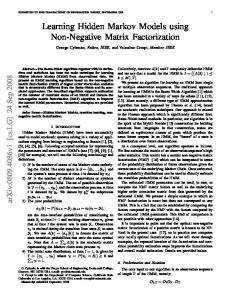
Figure 3. Two HSMMs are trained: One for failure sequences and one for non-failure sequences. Sequences consist of errors A, B, or C that have occurred in previously recorded training data. Failure sequences consist of errors that occurred within a time window of length ∆td preceding a failure (▲) by lead time ∆tl . Non-failure sequences consist of errors that occurred at times when no failure was imminent.
computing, hidden Markov models have been applied for the detection of intrusion into computer systems [33], fault diagnosis [7], or network traffic modeling [27]. Hidden Markov models have been extended to hidden semi-Markov models by several researchers. However, since most of these extensions have been developed for speech recognition, they are not appropriate for our purpose. An overview of previous extensions and a detailed description of our model are presented in [25].
Once the two models are trained, new unknown sequences can be evaluated if they indicate an upcoming failure or not. To achieve this, sequence likelihood is computed for both models and Bayes decision theory is applied in order to yield a classification (see Figure 4).
3.1. Approach Error event timestamps and message IDs form an eventdriven temporal sequence, which will from now on be called error sequence. HSMM failure prediction applies machine learning techniques in order to algorithmically identify characteristic properties indicating whether a given error sequence is failure-prone or not. More specifically, we adjust the model’s parameters using recorded error logs for which it is clear when failures have occurred. The trained hidden semi-Markov models are then applied in order to classify new error sequences as failure-prone or not failureprone. In machine learning, such approach is called “offline supervised learning”. After some data preprocessing including techniques such as tupling [30], failure and non-failure error sequences are extracted. Failure sequences consist of errors that have occurred within a time window of length ∆td preceding a failure by lead time ∆tl . Non-failure sequences consist of errors appearing in the log when no failures have occurred (see Figure 3). Two HSMMs are trained: One for failure sequences and the other for non-failure sequences. The main goal of training is that the failure model specifies characteristics of failure sequences —the non-failure model stays rather unspecific and is only needed for sequence classification.
Figure 4. Online failure prediction. At the occurrence of error A (present time), the sequence under investigation consists of all errors that have occurred within the preceding time window of length ∆td . Failure prediction is performed by computing sequence likelihood of the sequence using both the failure and non-failure model. Both likelihoods are evaluated using Bayes decision theory for classification as failure-prone or failure-free
The key notion of this approach to failure prediction is as follows: by training, the failure model has learned how error sequences look like if they precede a failure by lead time ∆tl . Hence, if a sequence under consideration is very similar to failure sequences in the training data, it is assumed
Figure 5. An exemplary HSMM as it is used for failure prediction. It consists of N-1 states that can generate error symbols A, B, or C, plus a final absorbing state that can generate failure symbol F. gij (t) indicate state transition distributions.
that a failure is looming which will occur at time ∆tl ahead. Of course, error sequences are rarely identical. Therefore, a probabilistic approach is needed in order to handle similarity, which in our case is achieved by use of hidden semiMarkov models.
tributions such that gij (t) = pij
R X r=0
Hidden Semi-Markov Models (HSMMs) are a continuous-time extension to hidden Markov models, which in turn are an extension to discrete time Markov chains (DTMC). This section sketches the basic principle of our model, a more detailed treatment can be found in [25]. HSMMs are determined by several quantities. Let S = {si } denote the set of states, 1 ≤ i ≤ N . Let π = [πi ] denote the vector of initial state probabilities and G(t) = [gij (t)] an N × N matrix of cumulative state transition probability distributions over time with the following properties: X πi = 1 , and (2) i
wij,r κij,r (t|θij,r )
(4)
r=0
s.t. ∀ i, j :
3.2. Hidden Semi-Markov Models
R X
wij,r = 1
and
∀i :
N X
pij = 1
(5)
j=1
pij is the limiting weight for transitions from state i to state j corresponding to transition probabilities in DTMCs. For each transition from i to j, wij,r denotes the weight of the r-th kernel κij,r . Finally, κij,r (t|θij,r ) denotes a cumulative, continuous, parametric distribution over time t with parameters θij,r such as mean and variance in case of normal distributions. HSMMs are called “hidden” since it is assumed that only the generated symbols can be observed and that the state of the stochastic process is hidden from the observer. In the case of failure prediction, this property can be mapped onto the fundamental concepts of faults and errors: • Faults are by definition unobserved. Hence they correspond to the hidden states.
(3)
• Errors, which are the manifestation of faults, correspond to the manifestation of hidden states, which are observation symbols.
π and G define a continuous-time semi-Markov process of traversals through states S. Furthermore, let O = {ok }, 1 ≤ k ≤ M denote a finite set of discrete observation symbols. Each time the stochastic process enters a state, one such observation symbol is generated according to a state-dependent probability distribution bi (ok ). Observation probabilities for all states set up an N × M matrix B = [bi (k)] = [bik ]. In summary, an HSMM is completely defined by λ = (π, G(t), B). Our approach allows to use a great variety of cumulative, parametric, continuous distributions to be used for gij (t). Moreover, our approach allows to use mixtures of such dis-
Figure 5 shows an exemplary HSMM as used for failure prediction. It constitutes a left-to-right structure including “shortcut transitions” to increase flexibility of the model. The string of hidden states ends in a special hidden state representing a failure. We have adapted standard HMM algorithms such as Baum-Welch and Forward-Backward to train the models (i.e., adjust λ from a set of training sequences) and to efficiently compute sequence likelihood. The next two sections provide more details. Although the models need to be trained before they can be applied in order to perform online failure prediction, the prediction part is described first.
∀i
:
X j
lim gij (t) = 1
t→∞
The reason for this is that training shares some theory with prediction but adds some more concepts.
3.3. Failure prediction Assume that both the failure and non-failure model have been trained, i.e., parameters λF and λF¯ are set. The goal is to assess, whether a given observation temporal sequence (an error sequence) o = [o0 . . . oL ] is failure prone or not. As shown in Figure 4, the first step is to compute sequence likelihoods of o for both models, on which the sequence is subsequently classified as failure-free or failure-prone using Bayes decision theory.
Sequence likelihood is defined as the probability that a given model λ can generate observation sequence o: P (o|λ)=
P
s
QL
πs0 bs0 (o0 )
k=1
P (Sk =sk , dk =tk −tk−1 | Sk−1 =sk−1 ) bsk (ok )
(6)
where s = [sk ] denotes a sequence of states of length L + 1 and tk are the timestamps of the sequence. The sum over s denotes that all possible state sequences are investigated. However as is the case for standard HMMs, due to the sum over all possible state sequences s Equation 6 suffers from unacceptable complexity. The so-called forward algorithm solves this issue for standard HMMs by applying a dynamic programming approach (see, e.g., [23]). A similar algorithm can be derived for our HSMM: By assuming gii (t) = 0 and defining vij (dk )
= P (Sk = sj , dk = tk − tk−1 | Sk−1 = si ) if i 6= j gij (dk ) N X = (7) gih (dk ) if i = j 1 − h=1
to incorporate the case of remaining in the same state, the so-called forward variable α becomes: αk (i) = P (O0 O1 . . . Ok , Sk = si |λ) α0 (i) = πi bi (O0 ) αk (j) =
N X
(8) αk−1 (i) vij (tk − tk−1 ) bj (Ok )
i=1
(1 ≤ k ≤ L) and sequence likelihood can be efficiently computed by P (o | λ) =
N X i=1
αL (i)
(9)
Sequence classification. Bayes decision theory proves that the error of misclassification is minimized if a sequence is assigned to the class of maximum posterior probability. However, in real failure prediction applications there are several things that have to be accounted for: 1. Likelihood P (o | λ) gets small very quickly for long sequences, such that limits of double-precision floating point operations are reached. For this reason, a technique called scaling and log-likelihoods have to be used. 2. Misclassification error is not always a good metric to evaluate classification. Rather, in real applications, different costs may be associated with classification. For example, falsely classifying a non-failure sequence as failure-prone might be much worse than vice versa. These issues can also be addressed by Bayes decision theory and the resulting classification rule is: Classify sequence o as failure-prone, iff � � � � log P (o | λF ) − log P (o | λF¯ ) > � � � � P (F¯ ) cF¯ F − cF¯ F¯ (10) + log log cF F¯ − cF F P (F ) | {z } | {z } ∈(−∞;∞)
const.
where cta denotes the associated cost for assigning a sequence of type t to class a, e.g., cF F¯ denotes the cost for falsely classifying a failure-prone sequence as failurefree. P (F ) and P (F¯ ) denote class probabilities of failure and non-failure sequences, respectively. See, e.g., [8] for a derivation of the formula. The right hand side of Inequality 10 determines a constant threshold on the difference of sequence loglikelihoods. If the threshold is small more sequences will be classified as failure-prone increasing the chance of detecting failure-prone sequences. On the other hand, the risk of falsely classifying a failure-free sequence as failure-prone is also high. If the threshold increases, the behavior is inverse: more and more failure-prone sequences will not be detected at a lower risk of false classification for non-failure sequences.
3.4. Training We have adapted the Baum-Welch expectationmaximization algorithm [3, 23] for this purpose. The objective of the training algorithm is to optimize the HSMM parameters π, G(t), and B such that the overall training sequence likelihood is maximized. From this approach follows, that the basic model topology (number of states, available transitions between states, number of observation symbols, etc.) must be pre-specified.
In analogy with the standard HMM training algorithm, a backward variable β is defined as: βk (i) = P (Ok+1 . . . OL | Sk = si , λ)
Training complexity is difficult to estimate since the number of iterations can hardly be estimated. One iteration has complexity O(N 2 L). However, training time is not as critical as it is not performed during system runtime.
βL (i) = 1 βk (i) =
N X
(11) vij (dk ) bj (Ok+1 ) βk+1 (j)
j=1
Using α and β together, ξ can be computed: ξk (i, j) = P (Sk = si , Sk+1 = sj | o, λ) ξk (i, j) = PN
i=1
αk (i) vij (dk+1 ) bj (Ok+1 ) βk+1 (j) PN α (i) vij (dk+1 ) bj (Ot+1 ) βk+1 (j) j=1 k
(12) (13)
which is the probability that a transition from state i to state j takes place at time tk . α, β and ξ can be used to maximize the model parameters. Re-estimation of π, and B is equivalent to standard HMMs, whereas re-estimation of pij , wij,r , and θij,r is based on the following principle: ξk (i, j) not only assigns a weight to the transition from i to j, as is the case for standard HMMs, but also assigns a weight to the duration of the transition. More precisely, each transition i → j can in principle account for all transition durations tk+1 − tk in the training sequences, each weighted by ξk (i, j). Hence transition parameters can be optimized iteratively such that they best represent the weighted durations. The entire procedure —computation of α, β and ξ— and subsequent maximization of model parameters is iterated until convergence. It can be proven that the procedure converges at least to a local maximum. Since it starts from a randomly initialized HSMM, the algorithm is performed several times with different initializations and the best model is kept for prediction. In order to avoid overfitting, i.e., the models memorize the training data set very well but perform badly on new, unknown data, we use background distributions for both B and G(t). Since size and topology of the model are not optimized by the Baum-Welch algorithm, several configurations of the principle structure shown in Figure 5 have to be tried.
3.5. Computational complexity With respect to online prediction the forward algorithm has to be executed twice: one time for the model of failureprone sequences and one time for the non-failure sequence model. Although the standard HMM forward algorithm belongs to complexity class O(N 2 L) where N is the number of hidden states and L is the length of the symbol sequence, We use a left-to-right model which limits complexity to O(N L), although the constant factors are larger than for standard HMMs since cumulative distributions need to be evaluated.
4. Models Used for Comparison We have compared our HSMM failure prediction approach to three other approaches: Dispersion Frame Technique and eventset-based method, which also operate on the occurrence of errors, and a straightforward reliability-based prediction algorithm, which evaluates previous occurrences of failures.
4.1. Reliability-based prediction As can be seen from Equation 1, failures can be predicted by reliability assessment during runtime. Due to the lack of insight into the system, we had to use a rather simple reliability model that assumes a Poisson failure process and hence approximates reliability by an exponential distribution: F (t) = 1 − e−λt (14) The distribution is fit to the short-term behavior of the system by setting the failure rate to the inverse of mean-timeto-failure (MTTF). We have set MTTF to the mean value observed in the data set used to assess the predictive accuracy of the technique. This yields an optimistic assessment of predictive accuracy since in a real environment, MTTF must be estimated from the training data set. A failure is predicted according to the median of the distribution. After each failure that occurs in the test data set, the timer is reset and prediction starts again. This is why this simple failure prediction method is based on runtime monitoring. Please note that we included such simple failure prediction model only for a rough assessment of failure-based prediction approaches and to get an idea what level of failure prediction quality can be obtained with a very simple approach. On the other hand, Brocklehurst and Littlewood [4] argue that none of the reliability models are really accurate, which is especially true for online short-term predictions.
4.2. Dispersion Frame Technique (DFT) DFT is a well-known heuristic approach to analyze a trend in error occurrence frequency developed by Lin [17] and published later by Lin and Siewiorek [18]. In their paper, the authors have shown that DFT is superior to classic statistical approaches like fitting of Weibull distribution shape parameters. A Dispersion Frame (DF) is the interval time between successive error events. The Error Dispersion Index (EDI)
is defined to be the number of error occurrences in the later half of a DF. A failure is predicted if one of five heuristic rules fires, which account for several system behaviors. For example, one rule puts a threshold on error-occurrence frequencies, another one on window-averaged occurrence frequency. Yet another rule fires if the EDI is decreasing for four successive DFs and at least one is half the size of its previous frame. If the predicted failure is closer to present time than warning time ∆tw , the prediction has been eliminated. In order to adjust the parameters we optimized each parameter separately. If two choices were almost equal in precision and recall, we took the one with fewer false positives.
4.3. Eventset-based Method Vilalta et al. from IBM Research at T.J. Watson proposed a prediction technique that is based on sets of events preceding a target event [31, 32]. In our case events correspond to errors and target events to failures. Since the authors did not consider any lead time, we had to alter the approach such that the events forming an eventset had to occur at least ∆tl before the failure. An eventset is formed from all error types occurring within the time window (see Figure 6).
The database DB of indicative eventsets is algorithmically built by procedures known from data mining. Going through the training dataset, two initial databases are formed: a failure database containing all eventsets preceding failures and a non-failure database with eventsets that occurred between the failures. The database also contains all subsets of eventsets that occurred in the training data, which has – at least theoretically – cardinality of the power set. However by minimum support thresholding together with branch and bound techniques, cardinality can be limited. The goal is to reduce the database in several steps such that only most indicative eventsets stay in it. To achieve this, all eventsets that have support less than a minimum threshold are filtered out. The remaining eventsets are checked for their confidence, which is in this case the ratio of number of times an eventset occurred in the failure database in comparison to its overall occurrence. This step removes eventsets that occur frequently before failures but also between failures. Additionally, a significance test is performed that removes an eventset if the probability of occurrence in the failure database is similar to the probability of occurrence in the non-failure database. In a last filtering step all remaining eventsets are sorted according to their confidence and all eventsets that are more general and have lower confidence are removed: an eventset Zi is said to be more general than Zj if Zi ⊂ Zj .
5. Experiment Description
Figure 6. Eventset-based method. An eventset is the set of error types that have occurred within a time window of length ∆td preceding a failure (▲) by lead time ∆tl
The goal of the method is to set up a rule-based failure prediction system containing a database of indicative eventsets. For prediction, each time an error occurs, the current set of events Z is formed from all errors that have occurred within ∆td before present time. The database DB of indicative eventsets is then checked whether Z is a subset of any D ∈ DB. If so, a failure warning is raised at time ∆tl in the future.
All prediction techniques presented in this paper have been applied to data of a commercial telecommunication system, which main purpose is to realize a so-called Service Control Point (SCP) in an Intelligent Network (IN). An SCP provides services2 to handle communication related management data such as billing, number translations or prepaid functionality for various services of mobile communication: Mobile Originated Calls (MOC), Short Message Service (SMS), or General Packet Radio Service (GPRS). The fact that the system is an SCP implies that the system cooperates closely with other telecommunication systems in the Global System for Mobile Communication (GSM), but the system does not switch calls itself. It rather has to respond to a large variety of different service requests regarding accounts, billing, etc. submitted to the system over various protocols such as Remote Authentication Dial In User Interface (RADIUS), Signaling System Number 7 (SS7), or Internet Protocol (IP). The system’s architecture is a multi-tier architecture employing a component based software design. At the time when measurements were taken the system consisted of more than 1.6 million lines of code, approximately 200 2 so-called
Service Control Functions (SCF)
Figure 7. Number of errors per 100 seconds in part of the test data. Diamonds indicate occurrence of failures.
components realized by more than 2000 classes, running simultaneously in several containers, each replicated for fault tolerance.
5.1. Failure definition and input data According to [1], a failure is defined as the event when a system ceases to fulfill its specification. Specifications for the telecommunication system require that within successive, non-overlapping five minutes intervals, the fraction of calls having response time longer than 250ms must not exceed 0.01%. This definition is equivalent to a required four-nines interval service availability: srvc. req. w/i 5 min., tr ≤ 250ms total no. of srvc. req. w/i 5 min.
!
≥ 99.99%
Consider the following two examples for clarification: (a) A perfect failure prediction would achieve a one-toone matching between predicted and actual failures which would result in precision = recall = 1 and false positive rate = 0. (b) If a prediction algorithm achieves precision of 0.8, the probability is 80% that any generated failure warning is correct (refers to a true failure) and 20% are false warnings. A recall of 0.9 expresses that 90% of all actual failures are predicted (and 10% are missed). A false positive rate of 0.1 indicates that 10% of predictions that should not result in a failure warning are falsely predicted as failure-prone.
(15)
where tr denotes response time. Hence the failures predicted in this work are performance failures that occur when Equation 15 does not hold. System error logs have been used as input data. The amount of log data per time unit varies heavily, as can be seen in Figure 7. Training data contained 55683 (untupled) errors and 27 failures whereas test data had 31187 (untupled) errors and 24 failures. Figure 9 shows a histogram of time-between-failures (TBF) and autocorrelation of failure occurrence for the test data.
5.2. Metrics The models’ ability to predict failures is assessed by four metrics that have an intuitive interpretation: precision, recall, false positive rate and F-measure. Although originally defined in information retrieval these metrics are frequently used for prediction assessment and have been used in similar studies, e.g., [34]. • Precision: fraction of correctly predicted failures in comparison to all failure warnings • Recall: fraction of correctly predicted failures in comparison to the total number of failures. • F-Measure: harmonic mean of precision and recall
Predicted
Ai =
• False positive rate: fraction of false alarms in comparison to all non-failures.
Failure NonFailure
Truth Failure Non-failure True positive False positive (TP) (FP) False negative True negative (FN) (TN) (a)
Metric precision
Formula P p = T PT+F P
recall=true positive rate
r = tpr =
false positive rate F-measure
TP T P +F N P f pr = F PF+T N 2∗p∗r F = p+r
(b) Figure 8. Contingency table (a) and definition of metrics (b)
In order to estimate the metrics, predictions have been computed for the test data set which have then been compared to the true occurrence of failures and a contingency table has been created (c.f. Figure 8-a). The decision, whether a predicted failure co-incidents with a true failure is based
1.0
0.006
0.6
0.8
0.004
0.4
ACF
0.002
200
400
600
800
0.0
0.2
0.000
Density
0
0
50
TBF [min]
100
150
200
250
300
Lag [min]
Figure 9. Left: Histogram of time between failures (TBF). Right: autocorrelation of failure occurrence.
on prediction period: if a true failure occurs within the timeinterval of length ∆tp starting at the predicted time of failure occurrence, the prediction is counted as true positive. We used a prediction period of ∆tp = 60s. All four metrics can then be computed from the contingency table using the formulas provided by Figure 8-b.
There is often an inverse proportionality between high recall and high precision. Improving recall in most cases lowers precision and vice versa. The same holds for true positive rate (which is equal to recall) and false positive rate: Increasing true positive rate also increases false positive rate. One of the big advantages of the HSMM method in comparison to the other techniques presented here is that it involves a customizable threshold for classification (c.f., Equation 10). By varying this threshold, the inverse proportionality can be controlled. From this follows that the contingency table looks different for each threshold value and hence also the four metrics change. It is common in this case to visualize precision and recall by a precision/recall plot, and true positive vs. false positive rate by a so-called ROC plot.
In order to compare computational complexity of the approaches, we measured computation times. This does not substitute a complexity analysis but since all algorithms have been run on the same machine processing the same data set, the numbers can be used to compare the different approaches. Specifically, we measured —if appropriate— training time and testing time. Testing time refers to the amount of time needed to process the entire test data in batch mode, which means that the next error is processed immediately after computations for the previous have finished, and not with the delays as they have occurred in the original log.
6. Results In this section, we present results based on applying the presented failure prediction methods to real data of the industrial telecommunication system. The section is structured along the approaches ordered by complexity of the approaches. In the following the term prediction performance is used to denote the overall ability to predict failures as expressed by precision, recall, F-measure and false positive rate (FPR) rather than the number of predictions per time unit.
6.1. Reliability model based prediction The reliability model-based failure prediction approach is rather simple and has been included to provide sort of a “lower bound” to show what prediction performance can be achieved with nearly no effort. Not surprisingly, prediction performance is low: Precision equals 0.214, recall 0.154 yielding an F-measure of 0.1791. Since the approach only issues failure warnings (there are no nonfailure-predictions), false positive rate cannot be determined, here. The reason why this prediction method does not really work is that the prediction method is almost periodic: after the occurrence of a true failure, the next failure is predicted at constant time to occur at the median of a distribution that is not adapted during runtime. However, it can be seen from the histogram of time-between-failures that the distribution is wide-spread (Figure 9-a) and from the auto-correlation of failure occurrence that there is no periodicity evident in the data set (Figure 9-b). Since “training” only comprises computation of the mean of time-between-failures, we did not report “training time”. The same holds for prediction time.
0.04 0.03 0.02
Density
0.01 0.00
20
40
60
80
number of symbols
(a)
(b)
Figure 10. Histogram of length of sequences (a) and histogram of delays between errors (b).
6.2. Dispersion Frame Technique Comparing the results of DFT with the original work by Lin and Siewiorek, prediction performance was worse. The main reason for that seems to be the difference of investigated systems: While the original paper investigated failures in the Andrews distributed File System based on the occurrence of host errors, our study applied the technique to errors that had been reported by software components in order to predict upcoming performance failures. In our study, intervals between errors are much shorter (c.f. Figure 10-b). Since DFT predicts a failure half of the length of the dispersion frame ahead, the method rather seldomly predicted a failure far ahead from present time. Since initial results for DFT were quite bad, we modified the thresholds for tupling and for the rules to yield better results. The best combination of parameters we could find resulted in a precision of 0.314, recall of 0.458, F-measure of 0.3729 and FPR of 0.0027. Since there is no real “training”, we have not reported training time. Running the algorithm on the entire test data set resulted in a computation time of four seconds.
6.3. Eventset-based method Construction of the rule database for the eventset-based method includes the choice of four parameters: length of the data window, level of minimum support, level of confidence, and significance level for the statistical test. We have run the training algorithm for all combinations of various values for the parameters and have selected the optimal combination with respect to F-measure. Best results have been achieved for a window length of 30s, confidence of
10%, support of 50% and significance level of 3σ yielding a recall of 0.917, precision of 0.242, F-measure of 0.3826, and FPR of 0.1068. This means that the prediction algorithm was able to predict almost all failures of the test data set. However, the problem with the approach is precision: only 24.2% of failure warnings are correct and 75.8% are false alarms. We have also tried to set parameters such that precision and recall become more equal but with no success: recall has been reduced dramatically without substantial improvement in precision. Training took 25s for one specific parameter setting and training time was mainly determined by the a-priori algorithm used for initial database construction. Performing rule checking on the test database took 9s. Our explanation for the results of the eventset-based method is that for the data of the telecommunication system checking solely for the occurrence of error types is not sufficient. It seems as if our basic assumption holds that error patterns need to be considered in order to reliably identify imminent failures.
6.4. Hidden Semi-Markov Models For the experiments we used Hidden Semi-Markov Models with N = 100 states and shortcuts leaping up to five states. The number N has been determined by the length of sequences, of which a histogram is shown in Figure 10-a. Probabilities π have been initialized in a linearly decreasing way such that the first state receives maximum weight and state N receives no initial weight, and then π is adapted by the training algorithm. In order to determine transition duration distributions, we have investigated the distribution of time between errors.
0
5
10
+
15
exponential quantiles
(a)
100
150
+
50 0
+ ++++++++ + + ++++++++++++++++++++++++++++++++++++++++++++++++++++++
data quantiles
150 100 50 0
data quantiles
+
+ + +++++ +++++++++ 0
50
100
150
exponential mixed with uniform
(b)
Figure 11. QQ-plot of delays between error symbols. (a) plotted against exponential distribution (b) plotted against exponential distribution mixed with uniform distribution
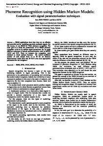
Figure 10-b shows a histogram. Most interestingly, by first visual impression the distribution seems to resemble an exponential distribution. Nevertheless, we have investigated various distributions by QQ plots. It turned out that the exponential distribution really yields the best fit. However, the exponential does not fit well in the tail of the distribution. To accommodate for this we have used an exponential distribution with uniform background to account for the tail resulting in a sufficiently good fit. Due to space restrictions, we can only present QQ plots comparing delay distribution with the pure exponential and exponential with background distribution in Figure 11. Other distributions such as lognormal resulted in significant deviations. Regarding observation background distributions we have chosen a distribution reflecting occurrence probability within the entire data set. As mentioned before, one of the advantages of our HSMM approach is that it allows to employ a customizable threshold permitting to control the tradeoff between, e.g., precision and recall. For this reason, we do not report single values for the metrics but provide two plots: a Precision-Recall plot and a ROC curve (see Figure 12). For each point in the Precision-Recall plot, an F-value can be computed resulting in F-measures ranging up to 0.7419. As might have been expected from the description of our approach, computing times for our HSMM method are longer than for the other methods: training the two HSMM models took 47s and predicting the data set took 15s.
7. Conclusions We have introduced a new approach to online failure prediction that forecasts the occurrence of failures by recogni-
tion of failure-prone patterns of error events. The prediction model builds on Hidden Semi-Markov Models. In order to compare results, we selected Dispersion Frame Technique (DFT) by Lin and Siewiorek, which evaluates the time when errors have occurred and the eventset-based method introduced by Vilalta et al., which applies data mining techniques on types of errors. As third comparison we have used a reliability model-based failure prediction approach that operates on the occurrence of failures only. All four models have been applied to field data of a commercial telecommunication system and results have been reported in terms of precision, recall, F-measure, and false positive rate. Our experiments have shown a natural correlation of the complexity of prediction approaches and the results that can be achieved: The reliability model based approach is simplest since it analyzes the least amount of information requiring almost no computation power – but it results in very poor prediction. DFT is a bit more complex and analyzes a little more data as only last few error messages are taken into account when checking several heuristic rules. This leads to better prediction results. The third method, the eventset-based method, applies a complex analysis using data mining techniques on a training data set. The method investigates sets of error types that have occurred within a time window. Hence the method builds on more detailed information resulting in an astonishing recall of 0.91. However, the method tends to warn frequently about an upcoming failure even if this is not the case: approximately three fourth of warnings are false alarms. Therefore, precision is rather low. Our HSMM approach is more complex investigating both time and type of error messages, which turns them into temporal sequences of error events. We use hidden semi-Markov models which require more complex computations. On the other hand, our HSMM approach out-
Figure 12. Prediction performance of the HSMM approach. precision-recall plot (left) and ROC curve (right). The various symbols denote different classification threshold values
Prediction technique
Precision
Recall
F-Measure
FPR
reliability-based
0.214
0.154
0.1791
n/a
DFT
0.314
0.458
0.3729
0.0027
Eventset
0.242
0.917
0.3826
0.1068
HSMM (max. F-measure)
0.852
0.657
0.7419
0.0145
Figure 13. Summary of prediction results performs the other approaches significantly. For example, for the maximum F-value of 0.7419, it achieves precision of 0.85 and recall of 0.66. Furthermore, our approach allows to employ a customizable threshold by which the tradeoff between, e.g., precision and recall can be controlled. Acknowledgments This work was supported by Intel Corporation and Deutsche Forschungsgemeinschaft DFG. We would also like to thank the authors and maintainers of GHMM at Max Planck Institute for Molecular Genetics for providing us with an efficient open source implementation of hidden Markov models and support.
References [1] A. Avižienis, J.-C. Laprie, B. Randell, and C. Landwehr. Basic concepts and taxonomy of dependable and secure computing. IEEE Transactions on Dependable and Secure Computing, 1(1):11–33, 2004.
[2] O. Babaoglu, M. Jelasity, A. Montresor, C. Fetzer, S. Leonardi, van Moorsel A., and M. van Steen, editors. Self-Star Properties in Complex Information Systems, volume 3460 of Lecture Notes in Computer Science. SpringerVerlag, 2005. [3] L. E. Baum, T. Petrie, G. Soules, and N. Weiss. A maximization technique occurring in the statistical analysis of probabilistic functions of Markov chains. Annals of Mathematical Statistics, 41(1):164–171, 1970. [4] S. Brocklehurst and B. Littlewood. New ways to get accurate reliability measures. IEEE Software, 9(4):34–42, 1992. [5] A. Brown and D. A. Patterson. To err is human. In Proceedings of the First Workshop on Evaluating and Architecting System dependabilitY (EASY ’01), Göteborg, Sweden, Jul. 2001. [6] A. Csenki. Bayes predictive analysis of a fundamental software reliability model. IEEE Transactions on Reliability, 39(2):177–183, Jun. 1990. [7] A. Daidone, F. Di Giandomenico, A. Bondavalli, and S. Chiaradonna. Hidden Markov models as a support for diagnosis: Formalization of the problem and synthesis of
[8] [9]
[10]
[11]
[12]
[13]
[14]
[15] [16]
[17]
[18]
[19]
[20]
[21] [22]
[23]
the solution. In IEEE Proceedings of the 25th Symposium on Reliable Distributed Systems (SRDS 2006), Leeds, UK, Oct. 2006. R. O. Duda, P. E. Hart, and D. G. Stork. Pattern Classification. Wiley-Interscience, 2 edition, 2000. W. Farr. Software reliability modeling survey. In M. R. Lyu, editor, Handbook of software reliability engineering, chapter 3, pages 71–117. McGraw-Hill, 1996. S. Garg, A. Puliafito, M. Telek, and K. Trivedi. Analysis of preventive maintenance in transactions based software systems. IEEE Trans. Comput., 47(1):96–107, 1998. S. Garg, A. van Moorsel, K. Vaidyanathan, and K. S. Trivedi. A methodology for detection and estimation of software aging. In Proceedings of the 9th International Symposium on Software Reliability Engineering, ISSRE 1998, Nov. 1998. I. Gertsbakh. Reliability Theory: with Applications to Preventive Maintenance. Springer-Verlag, Berlin, Germany, 2000. K. Hätönen, M. Klemettinen, H. Mannila, P. Ronkainen, and H. Toivonen. Tasa: Telecommunication alarm sequence analyzer, or: How to enjoy faults in your network. In IEEE Proceedings of Network Operations and Management Symposium, volume 2, pages 520 – 529, Kyoto, Japan, Apr. 1996. G. A. Hoffmann and M. Malek. Call availability prediction in a telecommunication system: A data driven empirical approach. In Proceedings of the 25th IEEE Symposium on Reliable Distributed Systems (SRDS 2006), Leeds, United Kingdom, Oct. 2006. P. Horn. Autonomic computing: IBM’s perspective on the state of information technology, Oct. 2001. D. Levy and R. Chillarege. Early warning of failures through alarm analysis - a case study in telecom voice mail systems. In ISSRE ’03: Proceedings of the 14th International Symposium on Software Reliability Engineering, Washington, DC, USA, 2003. IEEE Computer Society. T.-T. Y. Lin. Design and evaluation of an on-line predictive diagnostic system. PhD thesis, Department of Electrical and Computer Engineering, Carnegie-Mellon University, Pittsburgh, PA, Apr. 1988. T.-T. Y. Lin and D. P. Siewiorek. Error log analysis: statistical modeling and heuristic trend analysis. IEEE Transactions on Reliability, 39(4):419–432, Oct. 1990. C. Mundie, P. de Vries, P. Haynes, and M. Corwine. Trustworthy computing. Technical report, Microsoft Corp., Oct. 2002. F. A. Nassar and D. M. Andrews. A methodology for analysis of failure prediction data. In IEEE Real-Time Systems Symposium, pages 160–166, 1985. D. of Defense. MIL-HDBK-217F Reliability Prediction of Electronic Equipment. Washington D.C., 1990. J. Pfefferman and B. Cernuschi-Frias. A nonparametric nonstationary procedure for failure prediction. IEEE Transactions on Reliability, 51(4):434–442, Dec. 2002. L. R. Rabiner. A tutorial on hidden Markov models and selected applications in speech recognition. Proceedings of the IEEE, 77(2):257–286, Feb. 1989.
[24] F. Salfner. Predicting failures with hidden Markov models. In Proceedings of 5th European Dependable Computing Conference (EDCC-5), pages 41–46, Budapest, Hungary, Apr. 2005. Student forum volume. [25] F. Salfner. Modeling event-driven time series with generalized hidden semi-Markov models. Technical Report 208, Department of Computer Science, Humboldt-Universität zu Berlin, Germany, 2006. Available at http://edoc.hu-berlin.de/docviews/ abstract.php?id=27653. [26] F. Salfner, M. Schieschke, and M. Malek. Predicting failures of computer systems: A case study for a telecommunication system. In Proceedings of IEEE International Parallel and Distributed Processing Symposium (IPDPS 2006), DPDNS workshop, Rhodes Island, Greece, Apr. 2006. [27] P. Salvo Rossi, G. Romano, F. Palmieri, and G. Iannello. A hidden markov model for internet channels. In IEEE Proceedings of the 3rd International Symposium on Signal Processing and Information Technology (ISSPIT 2003), pages 50–53, Dec. 2003. [28] D. P. Siewiorek and R. S. Swarz. Reliable Computer Systems. Digital Press, Bedford, MA, second edition, 1992. [29] R. M. Singer, K. C. Gross, J. P. Herzog, R. W. King, and S. Wegerich. Model-based nuclear power plant monitoring and fault detection: Theoretical foundations. In Proceedings of Intelligent System Application to Power Systems (ISAP 97), pages 60–65, Seoul, Korea, Jul. 1997. [30] M. M. Tsao and D. P. Siewiorek. Trend analysis on system error files. In Proc. 13th International Symposium on FaultTolerant Computing, pages 116–119, Milano, Italy, 1983. [31] R. Vilalta, C. V. Apte, J. L. Hellerstein, S. Ma, and S. M. Weiss. Predictive algorithms in the management of computer systems. IBM Systems Journal, 41(3):461–474, 2002. [32] R. Vilalta and S. Ma. Predicting rare events in temporal domains. In Proceedings of the 2002 IEEE International Conference on Data Mining (ICDM’02), pages 474–482, Washington, DC, USA, 2002. IEEE Computer Society. [33] C. Warrender, S. Forrest, and B. Pearlmutter. Detecting intrusions using system calls: alternative data models. In IEEE Proceedings of the 1999 Symposium on Security and Privacy, pages 133–145, 1999. [34] G. Weiss. Timeweaver: A genetic algorithm for identifying predictive patterns in sequences of events. In Proceedings of the Genetic and Evolutionary Computation Conference, pages 718–725, San Francisco, CA, 1999. Morgan Kaufmann.