Using Immersive Virtual Reality to Study Hurricane Cases Duanjun Lu*, Paul J. Croft, R.S.Reddy Jackson State University, Jackson, MS Sean Ziegeler, Robert J. Moorhead Mississippi State University, Starkville, MS 1. INTRODUCTION
2. METHODS
Visualization may be applied in both an analytic and diagnostic manner to assess the behavior of the atmosphere. Meteorological visualization tools have evolved from static two-dimensional overlays to timelapse series with three-dimensional features. To fully realize the benefits of atmospheric modeling and better understand the physical processes in the atmosphere, an immersive visualization system (Ziegeler et al. 2001) has been developed within the Jackson State University Meteorology Program.
The numerical forecast model used is the Navy's Coupled Ocean/Atmosphere Mesoscale Prediction System (COAMPS) (Hodur 1997). This system consists of a data quality control system, a multivariate optimum interpolation (MVOI) analysis (Baker 1992), a fully-compressible, non-hydrostatic atmospheric model and an incompressible, hydrostatic ocean model cast in terrain following sigma-z coordinates.
Such a virtual environment allows users to physically observe what happens in the atmosphere. This provides an improved understanding, analysis, and forecast of storm systems and their behavior, as well as gives discrete knowledge of their defining features and dynamics. The most common types of meteorological visualizations have been twodimensional plots, either simple cartesian or contour plots. The two-dimensional visualization of multilayer, time-series data makes it difficult to see all layers and time steps in a single image. Using 3D visualization and animation, one can easily view multi-layer, time-series data sets in a unified manner. Most 3D visualization techniques can be used to provide a visual understanding of the vertical structure of the atmosphere in any part of a domain. The 3D visualization, however, does share a common problem with 2D: a limit on the number simultaneous variables that can be displayed and resolved by the human viewer. In this study we use immersive visualization to explore the evolution of hurricane structure. Some research papers have been published on the study of hurricane evolution and its inner structure (Krishnamurti et al. 1995; Liu, et al. 1997). However, no one has gone inside of a hurricane to examine what precisely happens. Immersive visualization provides an opportunity to navigate through a hurricane and see through the clouds. In this study, we use the COAMPS model to simulate two hurricane cases, Dennis and Floyd, and transfer the model output to the visualization system to explore the evolution of hurricanes.
In this study only atmospheric model data are used. The model features explicit moist physics, and parameterizations for long and short wave radiation. The model runs over a two-nested domain both with 121x121x30 grid points (27km and 9km for outer and inner domain spacing). Four movable two-nested domains were applied to the simulation of Dennis due to its long life-cycle and track. The same strategy was used for hurricane Floyd with 7 domains used during its life-cycle simulation. 3. DATA AND NUMERICAL MODELING Hurricane Dennis (24 August 1999 to 7 September 1999) and Floyd (8 September 1999 to 17 September 1999) cover a nearly 26-day period. The COAMPS model was initialized using the 0000 UTC Navy's global model (NOGAPS) blending with radiosonde and surface observations. Incremental updates with a 12-hour interval were utilized from 2300 UTC August through 1712 UTC September 1999. Lateral boundary conditions were given by NOGAPS analyses every 6 hours. The 30 vertical sigma levels were set at 10, 30, 55, 90, 140, 215, 330, 500, 750, 1100, 1600, 2300, 3100, 3900, 4800, 5800, 6800, 7800, 8675, 9425, 10175, 10925, 11675, 12425, 13300, 14300, 16050, 19400, 24400 and 31050m. Climate data for roughness, ground wetness, 500 meter resolution land and sea temperature and 1 km land-use data were used in simulations. The terrain data was 20 km resolution for the outer domain and 1 km for inner domain. The output was 1 hour interval with sea level pressure, wind u-component, vcomponent, and w-component, temperature, water vapor pressure, geopotential height, rain water-, snow
* Corresponding author address: Duanjun Lu , Jackson State University, Dept. of Physics, Atmospheric Sciences, & General Science. Jackson, MS39217 e-mail:
[email protected].
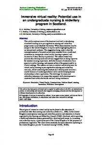
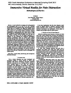
water-, ice water- and cloud water-mixing ratio available. Most observations were obtained from the NCAR web site, including surface and radisonde data. More complete datasets were obtained from the Marine Meteorology Division (MMD) of the Naval Research Laboratory (NRL) for the period 31 August through 7 September 1999. This data contained manual and automatic surface observation, fixed/mobile ship data, buoy, bogus, classified and unclassified raob data, aircraft reports and satellite data. The COAMPS model output was interpolated to height level. The visualization software VIS5D ( http://www.ssec.wisc.edu/~billh/vis5 d.html) was also used to display some results. 4. RESULT Hurricane track and intensity verification were made for the fine domains. The best track of the hurricane, the best minimum central pressure, and the best maximum 10-meter wind speeds were obtained from the National Hurricane Center. Note that the simulation is at 1-hour intervals while the observation is 6-hour interval. 4.1 Validation for the simulations Figure 1a compares the simulation and the best analysis tracks of Hurricane Dennis. The simulation reproduced the hurricane track very well, particularly after hurricane landfall. The simulation also reproduced the erratic path of the hurricane during the period 31 August to 3 September. The RMSE between the simulation and the best analysis was 140 km. The largest RMSE values occurred during the period when the hurricane moved erratically (nearly 160 km). The same analysis for Floyd's track is shown in Figure 1b. Compared with Dennis's erratic motion, Floyd moved fairly "straight". The simulation therefore showed very good agreement with observation, especially before Floyd weakened into a tropical storm (after 16 September). The overall RMSE of the track was about 130 km with a value as low as 90 km before 16 September. These errors are likely caused by the insufficient information in the large-scale initial conditions ingested into the model and the simulation center determination. The simulation center is determined from the point that has the minimum sea level pressure while the best analysis obtained the hurricane center position from several points observation.
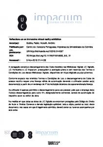
To demonstrate the model's capability in reproducing the deepening of hurricane Dennis and Floyd, we compared (see figure 2) the time series of the minimum central pressure and the maximum surface wind speed between the simulation and the best analysis. Although the simulated details were different from the analysis, the general trends of minimum sea level pressure and maximum surface winds were favorable for both cases. The best analysis showed a stronger hurricane intensity in sea level pressure and maximum surface winds. For example, COAMPS simulation provided the strongest intensity of hurricane Dennis on 29 August 1800 UTC with a central sea level pressure of 988 mb while the best analysis yielded a pressure of 962 mb on the same day. The best analysis indicated peak maximum surface winds on 29 August of 91 knots while the simulation gave a peak value of 67 knots on 31 August 0000 UTC for Dennis. It is noticed that, for sea level pressure and surface winds, the discrepancy between simulation and best analysis of Dennis tended to be decreased after 31 August. This is due to the model ingesting more complete observation data by using satellite, aircraft and buoys. Floyd reached its deepest intensity of 920 mb and its strongest surface winds of 135 knots on 13 September. On the other hand, the simulation yielded a weak hurricane with the minimum sea level pressure of 970 mb and maximum surface wind speed of 70 knots on the same day. The discrepancies between simulated and observed increased as both hurricanes intensified. The gap between the simulation and best analysis appeared to be biggest during the period when the hurricane reached its mature stage, and even filled when the actual hurricane was developing and weakening. Thus the model is not very good at the intensity verifications of a hurricane. 4.2 Visualization of the hurricanes In order to explore the inner structure of each hurricane, we compared the simulation and analysis through visualization. Figure 3a displays a NOAA-15 AVHRR multi-spectral image ( http://cimss.ssec.wisc.edu/tropic/archive/1999/storms/ dennis) at the mature stage of hurricane Dennis, while Figure 3b shows a top view of the hydrometeor fields as delineated by the 0.1g/kg isopleth of cloud water, rain water, snow water and ice water, and the sea level pressure from the simulation of 1 September 1200 UTC. It is obvious that the simulated general cloud distributions conform well to the satellite imagery. Both the model output and the observations showed
the development of organized spiral cloud bands with an echo-free eye in the central core. The sea level pressure also compared favorably to the hydrometeors field. For example, the area of the lowest sea level pressure values was located over the center of the simulated cloud. There was nearly no cloud around the low level center. The width of the hurricane eye in the simulation at this stage was larger than observed.
and Oceanography Center in Monterey through a Memorandum of Agreement.
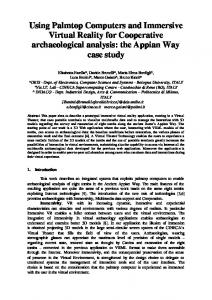
Figure 4 shows the spatial variation of the wind speed at 1 km on 0100 UTC 1 September. The eye and eye-wall were clearly revealed. A weak wind area was surrounded by the stronger spiral winds. The minimum value at the center was close to zero (0.3 m/s) while eye-wall region winds were 33 m/s. Figure 5a - 5e provides a 3D view of the equivalent potential temperature and winds at the surface and 7 km height. The equivalent potential temperature represents the static energy of air parcels and is conserved under the condition of inviscid, pseudoadiabatic flow.
Hodur, R. M., 1997: The navy research laboratory's coupled ocean/atmosphere mesoscale prediction system (COAMPS). Mon. Wea. Rev., 127, 858-878.
The 3D visualization of the equivalent potential temperature was for the 329K surface. This threshold value was based on the spatial variation of the winds. This surface separates the strong and weak winds. Some features that are associated with the eye, the eye wall and the spiral rain-bands are evident. The air trajectory analysis (not shown) showed that air parcels at lower level rotated and moved inward from the outer (high pressure) region. On the other hand, the asymmetric structure at the upper level was revealed. The air mass located in the northeast area appeared to ascend considerably, whereas the air over the southwest part appeared to descend.
7. REFERENCES Baker,N. L., 1992: Quality control for the U.S. Navy operational database. Wea. Forecasting, 7, 250261.
Krishnamurti, T. N., S. K. Bhowmik, D. Oosterhof, and G. Rohaly, 1995: Mesoscale signatures with the Tropics generated by physical initialization, Mon. Wea. Rev., 123, 2771-2790. Liu, Y., D-L. Zhang, and M. K. Yau, 1997: A mutiscale numerical study of hurricane Andrew (1992). Part I: explicit simulation and verification. Mon. Wea. Rev., 125,3073-3093. Ziegeler, S., R. J. Moorhead, P. J. Croft, and D. Lu, 2001: The MetVR case study: meteorological visualization in an immersive virtual environment. Preprint, IEEE Visualization 2001.
5. CONCLUSIONS A brief discussion of the simulation of two hurricanes, Dennis and Floyd, is presented. The COAMPS model output shows a good agreement between simulation and best analysis for both hurricane intensity and track. Visualization tools play a significant role in exploring the unique inner structure of the hurricanes. Some interesting pictures are presented above. More pictures, created by Vis5d and MetVR (an immersive virtual environment system), will be presented during the conference. 6. ACKNOWLEDGEMENT This research by the JSU Meteorology Program was supported by DoD's High Performance Visualization Center Initiative (HPVCI) through contract number N62306-99-D-B004. COAMPS was made available by the Fleet Numerical Meteorology
Figure 1. The center track of hurricane (a) Dennis and (b) Floyd from best analysis (circle-line) and simulation (star).
for cloud-, rain-, ice- and snow-water at 1200 UTC 1 September 1999.
Figure 4. Wind speed simulation on 1 km at 0100 UTC 1 September 1999.
Figure 2. Comparisons of minimum central sea level pressure and maximum surface winds for hurricane Dennis (a,b) and Floyd (c,d).
Figure 3. (a) Multispectral imagery at 1237 UTC 1 September 1999 and (b) a top view of the simulated hydrometeors, as determined by 0.1g/kg iso-surface
Figure 5. 3D view of simulated equivalent potential temperature surface (threshold potential surface value = 329 K) and winds at surface and 7 km on 1 September 1999 at (a) 0100 UTC, (b) 0600 UTC, (c) 1200 UTC, (d) 1800 UTC and (e) 2400 UTC.