Using the thermal Gaussian approximation for the ... - Semantic Scholar

THE JOURNAL OF CHEMICAL PHYSICS 125, 224104 共2006兲

Using the thermal Gaussian approximation for the Boltzmann operator in semiclassical initial value time correlation functions Jian Liu and William H. Millera兲 Department of Chemistry and K. S. Pitzer Center for Theoretical Chemistry, University of California, Berkeley, California 94720-1460 and Chemical Science Division, Lawrence Berkeley National Laboratory, Berkeley, California 94720-1460

共Received 6 September 2006; accepted 18 October 2006; published online 12 December 2006兲 The thermal Gaussian approximation 共TGA兲 recently developed by Frantsuzov et al. 关Chem. Phys. Lett. 381, 117 共2003兲兴 has been demonstrated to be a practical way for approximating the ˆ 兲 for multidimensional systems. In this paper the TGA is combined Boltzmann operator exp共−␤H with semiclassical 共SC兲 initial value representations 共IVRs兲 for thermal time correlation functions. Specifically, it is used with the linearized SC-IVR 共LSC-IVR, equivalent to the classical Wigner model兲, and the “forward-backward semiclassical dynamics” approximation developed by Shao and Makri 关J. Phys. Chem. A 103, 7753 共1999兲; 103, 9749 共1999兲兴. Use of the TGA with both of these approximate SC-IVRs allows the oscillatory part of the IVR to be integrated out explicitly, providing an extremely simple result that is readily applicable to large molecular systems. Calculation of the force-force autocorrelation for a strongly anharmonic oscillator demonstrates its accuracy, and calculation of the velocity autocorrelation function 共and thus the diffusion coefficient兲 of liquid neon demonstrates its applicability. © 2006 American Institute of Physics. 关DOI: 10.1063/1.2395941兴 I. INTRODUCTION

There is currently a great deal of effort focused on developing ways1–7 for adding quantum mechanical effects to classical molecular dynamics 共MD兲 simulations of chemical reactions, and other dynamical processes, in large molecular systems. Though purely classical MD simulations are adequate for many purposes, there is no doubt that quantum aspects of the dynamics will sometimes be important, and one will not know whether or not this is the case unless one has the ability of including them in the treatment, even if only approximately. Applications to a wide variety of molecular phenomena are obvious. Semiclassical 共SC兲 theory8–12 provides one way for adding quantum effects to classical MD simulations, and there is ample evidence that the SC approximation is a usefully accurate description of essentially all quantum effects in molecular dynamics.2,7,13–18 For systems with many degrees of freedom, various initial value representations 共IVRs兲 of SC theory provide the first step toward a practical way for carrying out SC calculations; this effectively replaces the nonlinear boundary value problem of traditional SC theory with a Monte Carlo average over the initial conditions of classical trajectories,9–12 a procedure much akin to what is done in classical MD simulations, allowing one to borrow from the great deal of computational development in that field. The added difficulty of a SC-IVR calculation, compared to a classical MD one, is the phase of the integrand, which carries all the quantum coherence information; thus all of the special techniques3–5,14,19,20 developed for carrying out SC-IVR calculations are concerned with this phase. a兲

Electronic mail: [email protected]

0021-9606/2006/125共22兲/224104/13/$23.00

In this paper we focus on two of simplest SC-IVRs, the “linearized” approximation to the SC-IVR 共LSC-IVR兲,3,6,14 which yields the “classical Wigner model,” and Shao and Makri’s simplified version of a forward-backward approximation to the SC-IVR, which they refer to as “forwardbackward semiclassical dynamics” 共FBSD兲.4,5 Both of these approaches deal with the “phase problem” by assuming that the two classical trajectories inherent to a time correlation function 共see Sec. II兲 are close to one another. The only remaining issue is the quantum Boltzmann operator which appears in a thermal correlation function 共see Sec. II兲. In the first applications of the linearized SC-IVR 共LSC-IVR兲共to reactive flux correlation functions, and thus reaction rates兲 the Boltzmann operator was approximated as harmonic about the saddle point 共transition state兲 on the potential surface;3 this worked fine so long as the temperature was not too low. She and Geva later developed a more general “local harmonic” approximation7 for the Boltzmann operator that allowed them to carry out very impressive LSC-IVR calculations for vibrational relaxation in liquids 共involving forceforce autocorrelation functions兲.7,21 Similarly, Poulsen et al. have used a variationally optimized local harmonic approximation6 for the Boltzmann operator in carrying out LSC-IVR calculations, and Bonella et al. have extended this latter approach to also be able to describe electronically nonadiabatic dynamics.22 More recently, Mandelshtam and co-workers have developed a very interesting thermal Gaussian approximation23,24 共TGA兲 for the Boltzmann operator. It is itself a SC approximation, based on Heller’s earlier “frozen Gaussian” approximation25 共except that it involves imaginary time propagation兲; it is also a type of local harmonic approxima-

125, 224104-1

© 2006 American Institute of Physics

Downloaded 14 Mar 2008 to 136.152.154.126. Redistribution subject to AIP license or copyright; see http://jcp.aip.org/jcp/copyright.jsp

224104-2

J. Chem. Phys. 125, 224104 共2006兲

J. Liu and W. H. Miller

tion, but one about the classically evolving trajectory 共in imaginary time兲. Hellsing et al. applied such approaches earlier,26 and more recently Shao and Pollak extended the TGA by showing how quantum corrections can be added to it.27 Other imaginary time SC approximations for the Boltzmann operator that have been applied to thermal time correlation functions are an imaginary Herman-Kluk-type SCIVR by Makri and Miller,28 and the imaginary time Van Vleck SC-IVR of Zhao and Miller.29 These latter two approaches provide more accurate approximations for the Boltzmann operator but are not as easy to implement as the TGA. The purpose of this paper is to use the TGA of Mandelshtam and co-workers within the LSC-IVR and FBSD approximations for thermal time correlation functions, to see how well it works and to demonstrate its potential for application to large molecular systems. Section II describes the SC-IVR theory of time correlation functions, including the LSC-IVR and the FBSD methods. A brief review of the TGA is given in Sec. III. Combinations of the TGA with the SCIVR methods 共TGA-LSC-IVR and TGA-FBSD兲 and their numerical advantages are discussed in Sec. IV. Several numerical applications of the TGA-LSC-IVR and TGA-FBSD methods are presented in Sec. V, including a strong anharmonic one-dimensional model system and a complex system 共liquid neon兲. Finally, some concluding remarks appear in Sec. VI.

Aˆ and Bˆ are operators relevant to the specific property of interest. The SC-IVR approximates the time evolution operator ˆ t/ប −iH e by a phase space average over the initial conditions of classical trajectories.9,10,32,33 The original, Van Vleck version of the IVR is ˆ

e−iHt/ប =

冕冕 dp0

dq0冑M qp/共2␲iប兲3NeiSt共p0,q0兲/ប兩qt典具q0兩, 共2.4兲

where 共q0 , p0兲 is the set of initial conditions 共i.e., coordinates and momenta兲 for a classical trajectory, 共pt共q0 , p0兲 , qt共q0 , p0兲兲 the phase point at time t which evolves from that trajectory, St共q0 , p0兲 the classical action along it, and M qp the determinant of the Jacobian matrix relating the final position and initial momentum, M qp = det共⳵qt共q0,p0兲/⳵p0兲.

For the correlation function in Eq. 共2.1兲 and 共2.2兲, one needs to insert two such representations of the evolution propagator, yielding the following double phase space average for the correlation function: CAB共t兲 = 共2␲ប兲−3NZ−1

II. SC-IVR CALCULATION OF TIME CORRELATION FUNCTIONS

Most quantities of interest in the dynamics of complex systems can be expressed in terms of time correlation functions.30 For example, dipole moment correlation functions are related to absorption spectra, flux correlation functions yield reaction rates, velocity correlation functions can be used to calculate diffusion constants, and vibrational energy relaxation rate constants can be expressed in terms of force correlation functions. The standard real time correlation function is of the form 1 ˆ ˆ ˆ CAB共t兲 = Tr共e−␤HAêiHt/បBê−iHt/ប兲 Z ˆ

ˆ

= Tr共␳ˆ 0AêiHt/បBê−iHt/ប兲,

共2.1兲

or sometimes it is convenient to use the following symmetrized version:31 1 ˆ ˆ ˆ ˆ CAB共t兲 = Tr共e−␤H/2Aê−␤H/2eiHt/បBê−iHt/ប兲. Z

共2.2兲

ˆ is the 共time-independent兲 Hamiltonian for the sysHere H tem, which for large molecular systems is usually expressed in terms of its Cartesian coordinates and momenta ˆ + V共qˆ 兲, ˆ = 1 pˆ TM−1pˆ + V共qˆ 兲 = H H 0 2

共2.3兲

where M is the 共diagonal兲 mass matrix and pˆ and qˆ are the momentum and coordinate operators, respectively. Also, in ˆ Eqs. 共2.1兲 and 共2.2兲, Z = Tr e−␤H 共␤ = 1 / kBT兲 is the partition ˆ function, ␳ˆ 0 = e−␤H / Z is the equilibrium density operator, and

共2.5兲

⫻

冕

冕冕冕 dp0

dq0

dp0⬘

⬘ 兲1/2具q0兩Aˆ␤兩q0⬘典 dq0⬘共M qpM qp

⫻eiSt共p0,q0兲/បe−iSt共p0⬘,q0⬘兲/ប具qt⬘兩Bˆ兩qt典,

共2.6兲

ˆ ˆ ˆ where Aˆ␤ = e−␤HAˆ for Eq. 共2.1兲 or Aˆ␤ = e−␤H/2Aê−␤H/2 for Eq. 共2.2兲. The primary difficulty in evaluating this expression is the oscillatory character coming from the difference between the action integrals of the trajectories with initial conditions 共q0 , p0兲 and 共q0⬘ , p0⬘兲. One way to deal with this phase problem, proposed by Miller and co-workers,3,14 is to make the 共rather drastic兲 approximation of assuming that the dominant contribution to the double phase space average comes from phase points 共q0 , p0兲 and 共q0⬘ , p0⬘兲 that are close to one another. Changing to sum and difference variables,

¯p0 = 21 共p0 + p0⬘兲, ⌬p0 = p0 − p⬘,

¯q0 = 21 共q0 + q0⬘兲, ⌬q0 = q0 − q0⬘ ,

共2.7兲

and expanding all quantities in the integrand of Eq. 共2.6兲 to first order in ⌬p0 and ⌬q0 gives the LSC-IVR, or classical Wigner model for the correlation function, LSC-IVR 共t兲 = Z−1 CAB

冕冕 dp0

dq0Aw␤ 共q0,p0兲Bw共qt,pt兲, 共2.8兲

¯ 0 , ¯p0兲共i.e., the “bars” have been rewhere here 共q0 , p0兲 ⬅ 共q ␤ moved兲, and Aw and Bw are the Wigner functions corresponding to these operators,


224104-3

J. Chem. Phys. 125, 224104 共2006兲

Semiclassical time correlation functions

Ow共q,p兲 = 共2␲ប兲−3N ⫻eip

T⌬q/ប

冕

ˆ 兩q + ⌬q/2典 d⌬q具q − ⌬q/2兩O

具x兩q0,p0典 =

ˆ . That is, the integrals over ⌬p and ⌬q for any operator O 0 0 have become the two Fourier integrals that produce the Wigner functions of the two operators. Equation 共2.8兲, with the remaining 共single兲 phase space average, now has the form of the classical correlation function, the only difference being that the Wigner functions corresponding to operators Aˆ and Bˆ appear rather than the classical functions. The LSCIVR result in Eq. 共2.9兲, also termed the classical Wigner model, has been obtained by a variety of formulations, so the result itself is not new. What is interesting, though, is to realize that it is contained with the overall SC-IVR description, as a well-defined approximation to it. Calculation of the Wigner function for operator Bˆ in Eq. 共2.8兲 is usually straightforward; in fact, Bˆ is often a function only of coordinates or only of momenta, in which case its Wigner functions is simply the classical function itself. Calculating the Wigner function for operator Aˆ␤, however, involves the Boltzmann operator with the total Hamiltonian of the complete system, so that carrying out the multidimensional Fourier transform to obtain it is far from trivial. Furthermore, it is necessary to do this in order obtain the distribution of initial conditions of momenta p0 for the real time trajectories. A rigorous way to treat the Boltzmann operator is via a Feynman path integral expansion, but it is then in general not possible to evaluate the multidimensional Fourier transform explicitly to obtain the Wigner function for Aˆ␤ 共and thus the distribution of initial conditions of the momenta p0; Appendix A discusses and analyzes this situation in more detail兲. The inability to calculate the Wigner function of Aˆ␤ exactly is, in fact, the reason for the various harmonic and local harmonic approximations to the Boltzmann operator noted above, and the TGA discussed below in Sec. III. Another SC-IVR approach for the time evolution operaˆ tors e−iHt/ប is the Herman-Kluk, or coherent state IVR,12 ˆ

e−iHt/ប = 共2␲ប兲−3N

冕冕 dq0

dp0Ct共q0,p0兲eiSt共p0,q0兲/ប兩qt,pt典

⫻具q0,p0兩,

共2.10兲

where the preexponential factor is given by

冋冉

Ct共q0,p0兲 = 2−3N/2 det ⌫1/2 − 2iប⌫1/2

⳵qt −1/2 ⳵pt 1/2 ⌫ + ⌫−1/2 ⌫ ⳵q0 ⳵p0

⳵qt 1/2 1 −1/2 ⳵pt −1/2 ⌫ ⌫ − ⌫ ⳵p0 2iប ⳵q0

冊册

1/2

,

共2.11兲 and 兩q0 , p0典 and 兩qt , pt典 are coherent states, the wave functions for which are given by

2 ␲

冉

3N/4

共det ⌫兲1/4 exp − 共x − q0兲T⌫共x − q0兲

冊

i + pT0 共x − q0兲 . ប

共2.9兲

,

冉冊

共2.12兲

Here ⌫ is a 共positive definite兲 width matrix. Inserting two such Herman-Kluk representations for the propagator into Eq. 共2.1兲 and 共2.2兲 leads to the following double phase space average for the correlation function:

CAB共t兲 = 共2␲ប兲−3NZ−1 ⫻

冕

冕冕冕 dp0

dq0

dp0⬘

dq0⬘Ct共q0,p0兲C*t 共q0⬘,p0⬘兲

⫻具q0,p0兩Aˆ␤兩q0⬘,p0⬘典eiSt共p0,q0兲/ប ⫻e−iSt共p0⬘,q0⬘兲/ប具qt⬘,pt⬘兩Bˆ兩qt,pt典.

共2.13兲

The phase cancellation here is as severe in this integrand as it is in Eq. 共2.6兲. Shao and Makri4,5 introduced an approximate way to evaluate it by assuming that the dominant contribution to the double phase space average comes from two trajectories, one starting from 共q0 , p0兲 and another from 共q0⬘ , p0⬘兲, that satisfy the following “jumps” in coordinates and momenta at time t:

qt⬘ = qt − ប

⳵B共qt,pt兲 , ⳵pt

pt⬘ = pt + ប

⳵B共qt,pt兲 . ⳵qt

共2.14兲

This assumption yields the FBSD method for the correlation function,

FBSD 共t兲 = 共2␲ប兲−3NZ−1 CAB

冕冕再冉 dq0

dp0

1+

3N 2

冊

⫻具q0,p0兩Aˆ␤兩q0,p0典 − 2具q0,p0兩共xˆ − q0兲T

冎

⫻⌫Aˆ␤共xˆ − q0兲兩q0,p0典 B共qt,pt兲.

共2.15兲

The essential remaining task here is to evaluate the coherent state matrix elements of operator Aˆ␤, which is nontrivial because Aˆ␤ involves the Boltzmann operator with the total Hamiltonian of the complete system. This is analogous to the problem of computing the multidimensional Fourier transform to obtain the Wigner function for operator Aˆ␤ in the LSC-IVR approach described above. As in the LSC-IVR approach, if the Boltzmann operator is treated exactly, i.e., by Feynman path integration, the coherent matrix cannot be easily evaluated, as in necessary to obtain the distribution of initial conditions for the real time trajectories; Appendix A also discusses this in more detail. Just as for the LSC-IVR


224104-4

J. Chem. Phys. 125, 224104 共2006兲


approach, it is these various local harmonic approximations to the Boltzmann that allow these matrix elements 共or multidimensional Fourier transforms兲 to computed analytically and thus obtain an explicit result to the distribution of initial conditions 共q0 , p0兲 for the real time trajectories.

ˆ

具x兩e−␶H兩x⬘典 = =

冕冕冉冊 dq0

1 2␲

ˆ

具x兩e−␶H兩q0典 =

冉冊 1 2␲

冉

1 1 exp − 共x − q共␶兲兲T 2 兩det共G共␶兲兲兩1/2

冊

⫻G 共␶兲共x − q共␶兲兲 + ␥共␶兲 , −1

共3.1兲

where G共␶兲 is an imaginary time dependent 3N ⫻ 3N real symmetric and positive-definite matrix, q共␶兲 the center of the Gaussian, and ␥共␶兲 a real scalar function. The parameters are governed by the equations of motion: d G共␶兲 = − G共␶兲具ⵜⵜTV共q共␶兲兲典G共␶兲 + ប2M−1 , d␶

d q共␶兲 = − G共␶兲具ⵜV共q共␶兲兲典, d␶

共3.2兲

1 d ␥共␶兲 = − Tr共具ⵜⵜTV共q共␶兲兲典G共␶兲兲 − 具V共q共␶兲兲典, 4 d␶

冉冊

exp共2␥共␶/2兲兲兩det共G共␶/2兲兲兩

␶ 2

⫻G−1

␶ 2

T

G−1

exp −

x⬘ − q

␶ 2

␶ 2

1 ␶ x⬘ − q 2 2 .

T

共3.5兲

The expression for a partition function, for example, becomes Z= =

冕冕冕 dx

dq0

ˆ

ˆ

dq0具x兩e−␶H/2兩q0典具q0兩e−␶H/2兩x典

1 exp共2␥共␶/2兲兲 . 共4␲兲3N/2 兩det G共␶/2兲兩1/2

共3.6兲

Frantsuzov and Mandelshtam23 originally utilized the variational principle to obtain the equations of motion, Eq 共3.2兲. Shao and Pollak later rederived these equations by expanding the potential function in terms of the Gaussian averaged potential and its derivatives. In doing so, they showed the TGA to be a harmonic approximation about the imaginary time dependent path q共␶兲 and gave its more generalized version.27 In order to make it feasible to apply the TGA to complex systems, one must be able to evaluate the quantities 具V共q共␶兲兲典, 具ⵜV共q共␶兲兲典, and 具ⵜⵜTV共q共␶兲兲典 in Eq. 共3.2兲 efficiently. To do so, the potential is usually expressed as a sum of Gaussian functions or polynomial functions so that these quantities are evaluated analytically. Recent applications have shown the TGA to be a good approximation for the thermodynamics properties of some complex systems 共neon clusters兲 even at very low temperature.23,34

IV. SC-IVR METHODS WITH TGA

with the notation 1 具h共q兲典 = ␲

3N

1 ␶ x−q 2 2

⫻ x−q

III. THERMAL GAUSSIAN APPROXIMATION

3N/2

ˆ

冉冉冉冊冊冉冊冉冉冊冊冊冉冉冉冊冊冉冊冉冉冊冊冊

⫻exp −

For a N-particle system described in Eq. 共2.3兲, the thermal 共imaginary time兲 propagator 共i.e., coordinate representaˆ tion of the Boltzmann operator兲 e−␶H is approximated by Mandelshtam and co-workers as a multidimensional Gaussian form:23,24

ˆ

dq0具x兩e−␶H/2兩q0典具q0兩e−␶H/2兩x⬘典

3N/2

1 兩det共G共␶兲兲兩1/2

冕

⬁

dx共− 共x − q共␶兲兲T

−⬁

⫻G−1共␶兲共x − q共␶兲兲兲h共x兲.

共3.3兲

The initial conditions for the imaginary time propagation are q共␶ ⯝ 0兲 = q0,

The SC-IVR description of real time dynamics can be combined with any type of method for evaluating elements of Boltzmann operator what one uses for it is a question of accuracy and ease of application. Here we consider the TGA for the Boltzmann operator, showing how it leads to particularly simple ways for carrying out semiclassical dynamics calculations for complex systems with the two approximate SC-IVR’s, the LSC-IVR and the FBSD 共TGA-LSC-IVR or TGA-FBSD兲, summarized in the preceding section.

G共␶ ⯝ 0兲 = ប2␶M−1 ,

␥共␶ ⯝ 0兲 = − ␶V共q0兲.

共3.4兲

To ensure that the element of the Boltzmann operator ˆ 具x兩e−␶H兩x⬘典 is symmetric, Frantsuzov and Mandelshtam compound the approximation in Eq. 共3.1兲 twice to obtain

A. TGA-LSC-IVR

The TGA for the Boltzmann operator, Eq. 共3.5兲, makes it possible to analytically integrate out the phase term in the Wigner transform of the Boltzmann operator of the LSCIVR; i.e., substituting Eq. 共3.5兲 into Eq. 共2.9兲 gives


224104-5

J. Chem. Phys. 125, 224104 共2006兲


ˆ

关e−␤H兴w共x,p兲 = 共2␲ប兲−3N

冕冕冕

⬇ 共2␲ប兲−3N =

冕

ˆ

d⌬x具x − ⌬x/2兩e−␤H兩x + ⌬x/2典eip d⌬x

ˆ

ˆ

dq具x − ⌬x/2兩e−␤H/2兩q0典具q0兩e−␤H/2兩x + ⌬x/2典eip

1 ␲

3N/2

␤ 2

T

⫻exp − x − q

exp共2␥共␤/2兲兲 ␤ T p/ប2 1/2 exp − p G 兩det G共␤/2兲兩 2

G−1

␤ 2

x−q

␤ 2

1 Z ⫻

冕冕

冕

with the TGA, it is more convenient to use the symmetrized ˆ ˆ version Aˆ␤ = e−␤H/2Aê−␤H/2 if Aˆ = A共xˆ 兲 is a local operator; ˆ however, the form Aˆ␤ = e−␤HAˆ is preferred if Aˆ = pˆ , since ˆ evaluating derivatives of 具q0兩e−␤H/2兩x + ⌬x / 2典 with respect to q0 in Eq. 共4.1兲 would require considerably more work in the imaginary time propagation with the TGA, i.e., extra equations of motion for ⳵G共␶兲 / ⳵q0 , ⳵q共␶兲 / ⳵q0, etc., would be required in Eq 共3.2兲. Applying the TGA within Eq. 共2.9兲, TGALSC-IVR autocorrelation functions are expressed as

1 exp共2␥共␤/2兲兲 3N/2 共4␲兲兩det G共␤/2兲兩1/2

dp0

兩det G共␤/2兲兩1/2 ␤ ␤ TGA-LSC-IVR exp − pT0 G p0/ប2 f AA x0,p0,q ;t , 2 3N/2 共␲ប 兲 2 2

dx0

1 ␤ 3N/2 1/2 exp − x0 − q ␲ 兩det G共␤/2兲兩 2

冉冉冊冊共2兲

冉冊冊

␤ ;t = A共q0兲A共xt共x0,p0兲兲 2

共4.3兲

ˆ ˆ for local operators with Aˆ␤ = e−␤H/2A共xˆ 兲e−␤H/2, and

冉

TGA-LSC-IVR f AA

共3兲

冉冊冊冉冉冊冊冉冊

␤ x0,p0,q ;t 2

= pT0 pt共x0,p0兲 − iប x0 − q

␤ 2

T

G−1

␤ pt共x0,p0兲 2 共4.4兲

ˆ for the momentum operator Aˆ = pˆ with Aˆ␤ = e−␤Hpˆ . Monte Carlo 共MC兲 evaluation of Eq. 共4.2兲 for complex systems is now straightforward:

共1兲

冉冉冉冊冊冉冊冉冉冊冊冊冉冉冊冊

dq0

where TGA-LSC-IVR x0,p0,q f AA

共4.1兲

.

Equation 共4.1兲 contains no oscillatory term, so the integrand can be naturally used as the sampling function for Monte Carlo calculations of the LSC-IVR correlation functions of complex systems. In the high temperature limit, ␤ → 0, it is straightforward to verify that Eq. 共4.1兲 reduces to its classical limit, the classical Boltzmann distribution, which was also pointed out by Shao and Pollak27 by considering the limit ប → 0. To obtain the Wigner function for operator Aˆ␤ 关Eq. 共2.8兲兴

冉

T⌬x/ប

冉冊冉冉冊冊冉冉冉冊冊冉冊冉冉冊冊冊

dq0共2␲ប兲−3N

TGA-LSC-IVR CAA 共t兲 =

T⌬x/ប

Generate an imaginary time trajectory governed by the TGA equations of motion, Eq. 共3.2兲, the weight of which is sampled by the function exp共2␥共␤ / 2兲兲 / 兩det G共␤ / 2兲兩1/2.

T

G−1

␤ 2

x0 − q

␤ 2

共4.2兲

The imaginary time trajectory produces Gaussian distributions in both position and momentum spaces, exp共−共x0 − q共␤ / 2兲兲TG−1共␤ / 2兲共x0 − q共␤ / 2兲兲兲 and exp共 −pT0 G共␤ / 2兲p0 / ប2兲, respectively, which can be use to sample initial conditions 共x0 , p0兲 for the real time trajectory very efficiently. Run real time trajectories from phase space points 共x0 , p0兲 and estimate the property TGA−LSC−IVR 共x0 , p0 , q共␤ / 2兲 ; t兲 of the corresponding f AA time correlation function.

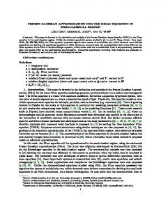
A schematic representation of Eq. 共4.2兲 for the TGALSC-IVR is given in Fig. 1. Provided that TGA−LSC−IVR f AA 共x0 , p0 , q共␤ / 2兲 ; t兲 does not vary rapidly, the MC sampling of Eq. 共4.2兲 is much more efficient for highdimensional system than one might expect. Our applications of the TGA-LSC-IVR to large systems show that only a few phase space points 共x0 , p0兲共i.e., real time trajectories兲 are necessary for each imaginary time trajectory to yield converged results so long as the number of imaginary time trajectories is sufficient to guarantee the convergence of the


224104-6

J. Chem. Phys. 125, 224104 共2006兲


thermodynamic properties. For example, when enough imaginary time trajectories have been propagated for the quantity 具p2典 to converge, only a few real time trajectories for each imaginary time trajectory are necessary to obtain the real time correlation function 具pT0 pt典 accurately. It should be noted that Morinica et al.35 have recently expressed the Wigner function of the Boltzmann operator using an imaginary time Gaussian wave packet approximation that, though formulated differently, can be shown to be equivalent to the TGA treatment 关i.e., Eq. 共4.1兲兴 and have used it to compute thermal time correlation functions. The essential difference of this work from the present is that Ref. 35 uses the Gaussian approximation to compute the Wigner function of the Boltzmann operator itself, and makes the further approximation that the Wigner function of operator Aˆ␤ is

FIG. 1. 共Color online兲 Schematic representation of the TGA-LSC-IVR representation of the density 共Boltzmann operator兲 for two particles. Black solid circles represent positions of two particles at the beginning and end of the imaginary time propagation, black curves indicate imaginary time trajectories, purple solid circles demonstrate Wigner density phase points generated upon imaginary time trajectories according to Eq. 共4.2兲, red wavy lines illustrate spring potentials 共from Gaussian distributions兲 between final points of imaginary time trajectories and phase points, and green straight lines depict intermolecular interactions. The generated phase points 共purple solid circles兲 are not involved in the intermolecular interaction directly in the imaginary time, which is different from that in Fig. 5 The schematic representation of the TGA-FBSD representation of the density 共Boltzmann operator兲 for two particles is exactly the same as that of the TGA-LSC-IVR, except that purple sold circles depict coherent state phase points and the corresponding Gaussian distribution parameters are different.

the product of the separate Wigner functions of the Boltzmann opertor and that of operator Aˆ. The TGA-LSC-IVR approach described above deals directly with the Wigner function of operator Aˆ␤.

B. TGA-FBSD

The Husimi transform of the Boltzmann operator,

conditions 共x0 , p0兲 for the real time trajectories. Using the TGA 关Eq. 共3.5兲兴 to approximate the Boltzmann operator allows the Husimi transform to be evaluated analytically, giving the following result:

ˆ

具x0 , p0 兩 e−␤H 兩 x0 , p0典, plays the analogous role in the FBSD method as the Wigner function of operator Aˆ␤ does in the LSC-IVR; i.e., it is the quantity used to sample initial

ˆ

具x0,p0兩e−␤H兩x0,p0典 =

冕冕 ⬘ 冕冕冕冕冉冊 dx

ˆ

dx 具x0,p0兩x典具x兩e−␤H兩x⬘典具x⬘兩x0,p0典

=

dq0

=

dq0

dx

1 2␲

ˆ

ˆ

dx⬘具x0,p0兩x典具x兩e−␤H/2兩q0典具q0兩e−␤H/2兩x⬘典具x⬘兩x0,p0典

3N/2

exp共2␥共␤/2兲兲兩det ⌫兩1/2 兩det G共␤/2兲兩兩det共⌫ + 共1/2兲G−1共␤/2兲兲兩

冉冉冉冊冊冊冉冉冉冊冊冉冊冉冉冊冊冉冉冊冊冊

1 ␤ ⫻exp − pT0 ⌫ + G−1 2 2 ⫻exp − x0 − q

␤ 2

T

G−1

−1

p0/2ប2

␤ 2

1 ␤ ⌫ + G−1 2 2

−1

⌫ x0 − q

␤ 2

.

共4.5兲

The integrand in Eq. 共4.5兲 can thus be used as the Monte Carlo sampling function for the real time initial conditions 共x0 , p0兲. One can show that Eq. 共4.5兲 reduces to its classical limit—the Boltzmann distribution—in the high temperature limit, ␤ → 0, i.e., when Eq. 共3.4兲 holds. Combining the TGA with the FBSD expression for the correlation 关Eq. 共2.15兲兴 gives the following TGA-FBSD result for correlation functions of complex systems: TGA-FBSD CAA 共t兲 =

1 Z ⫻ ⫻

冕冕冕

dq0

1 exp共2␥共␤/2兲兲 3N/2 共4␲兲兩det G共␤/2兲兩1/2

dx0

兩det ⌫兩1/2 exp共− 共x0 − q共␤/2兲兲TG−1共␤/2兲共⌫ + 共1/2兲G−1共␤/2兲兲−1⌫共x0 − q共␤/2兲兲兲 ␲3N/2兩det G共␤/2兲兩1/2兩det共⌫ + 共1/2兲G−1共␤/2兲兲兩1/2

dp0

exp共− pT0 共⌫ + 共1/2兲G−1共␤/2兲兲−1p0/2ប2兲 TGA-FBSD ␤ ;t , x0,p0,q 2 3N/2 −1 1/2 f AA 共2␲ប 兲兩det共⌫ + 共1/2兲G 共␤/2兲兲兩 2

冉

冉冊冊

共4.6兲


224104-7

where

J. Chem. Phys. 125, 224104 共2006兲


冉

TGA-FBSD f AA x0,p0,q

冉冊冊冋

冉冉冊冊冉冊冉冉冊冊冉冉冊冊冉冊冉冉冊冊冉冉冊冊冉冉冊冊册

3N 1 ␤ ␤ − x0 − q ;t = 1 + 2 2 2 2 −q

␤ 2

−

␤ 2

T

G−1

1 −1 ␤ 1 T 2 p0 ⌫ + G 2 2ប 2

1 ␤ ⌫ + G−1 2 2

−1

−1

1 ␤ ⌫ ⌫ + G−1 2 2

1 ␤ ⌫ ⌫ + G−1 2 2

␤ 2

−1

G−1

x0

−1

p0 A共q0兲A共xt共x0,p0兲兲

共4.7兲

ˆ ˆ for local operators with Aˆ␤ = e−␤H/2A共xˆ 兲e−␤H/2, and

冉

TGA-FBSD x0,p0,q f AA

冉冊冊冋冉冊冉冉冊冊冉冉冊冊冉冉冊冊冉冊冉冉冊冊冉冉冊冊冉冊冉冉冊冊册冉冉冊冉冉冊冊冉冊冉冉冊冊冉冉冊冊冊冉冊冉冉冊冊冉冉冊冊冉冉冊冉冉冊冊冊 ␤ ;t = 2

1+

3N 1 1 ␤ − 2 pT0 ⌫ + G−1 2 2 2ប 2

1 ␤ ⫻ ⌫ + G−1 2 2 1 ␤ ⫻ pTt G−1 2 2 1 ␤ + pTt G−1 2 2

−1

1 ␤ ⌫ ⌫ + G−1 2 2

1 ␤ ⌫ + G−1 2 2

1 ␤ ⌫ + G−1 2 2

ˆ for the momentum operator Aˆ = pˆ with Aˆ␤ = e−␤Hpˆ . To obtain better convergence, the partition function Z is calculated by using f TGA-FBSD共x , p , q共␤ / 2兲 ; t兲共Aˆ = 1兲 as the estimator for AA

0

−1

0

the Monte Carlo sampling. The Monte Carlo procedure for evaluating the TGAFBSD is similar to that of the TGA-LSC-IVR described in FBSD 共x0 , p0 , q共␤ / 2兲 ; t兲 the previous section. However, since f AA typically involves more cancellation than does the analogous quantity in the TGA-LSC-IVR, the number of real time trajectories required for each imaginary trajectory to obtain convergence is considerably larger than for the TGA-LSCIVR. A schematic representation of Eq. 共4.6兲 for the TGAFBSD is also given in Fig. 1, which is the same as that of the TGA-LSC-IVR. The TGA-LSC-IVR and the TGA-FBSD are, in fact, closely related to one another 共and give very similar results in most applications兲. For example, the Gaussian distributions in position and momentum are the same for the two approximations in the limit ⌫ → ⬁ in Eq. 共4.6兲 or 共4.5兲, provided one rescales p0 by the squared root of the matrix 共2⌫G共␤ / 2兲 + 1兲−1. Furthermore, the Wigner function and the Husimi function of the density with the TGA representation are equivalent in the limit ⌫ → ⬁, i.e., the coherent state becomes the position eigenstate, though, TGA-FBSD TGA-LSC-IVR 共x0 , p0 , q共␤ / 2兲 ; t兲 ⫽ f AA 共x0 , p0 , q共␤ / 2兲 ; t兲 f AA even in that limit. This arises from the fact that the FBSD density is not the same as the Husimi function 具x0 , p0兩␳ˆ 0兩x0 , p0典, but is instead 共1 + 共3N / 2兲兲具x0 , p0兩␳ˆ 0兩x0 , p0典 − 2具x0 , p0兩共xˆ − x0兲T⌫␳ˆ 0共xˆ − x0兲兩x0 , p0典, a narrower one. It is straightforward to show that both the TGA-LSC-IVR and the TGA-FBSD reduce to the classical limit at high temperature.

1 ␤ ⌫ ⌫ + G−1 2 2 −1

G−1

␤ 2

−1

p0 − iបpTt G−1

−1

1 ␤ ⌫ ⌫ + G−1 2 2

−1

p0 −

x0 − q

␤ 2

1 ␤ x0 − q 2 2

T

G−1

␤ 2

␤ 2

1 ␤ ⌫ + G−1 2 2

−1

p0 − iបG−1

−1

⌫ x0 − q

␤ 2

x0 − q

␤ 2

␤ 2

共4.8兲

V. NUMERICAL APPLICATIONS A. Anharmonic oscillator

The first example is a calculation of the force-force autocorrelation function for an asymmetric anharmonic oscillator, 1 V共x兲 = m␻2x2 − 0.10x3 + 0.10x4 , 2

共5.1兲

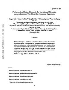
with m = 1 and ␻ = 冑2. This potential has been used as a test model and discussed previously in the literature.4,16,36 Both the LSC-IVR and the FBSD methods are able to describe the dephasing accurately for short times and semiquantitatively for longer times, but fail to capture the rephrasing at longer times due to coherence effects. In many cases in complex systems one expects such long time rephasing effects to be quenched by coupling among the various degrees of freedom.10,20,37 In order to explore how well the TGA-LSC-IVR and the TGA-FBSD perform, we test them at a high temperature ␤ប␻ = 冑2 / 10 and a very low temperature ␤ប␻ = 8冑2, comparing the results to the classical and the exact quantum results. At both temperatures, we use 21 imaginary trajectories with the imaginary time step of 0.01, and a large number of real time trajectories generated from each imaginary trajectories with a real time step of 0.02. The velocity Verlet integrator was used for both real and imaginary time dynamics. Figure 2 shows the force autocorrelation function at the temperature ␤ប␻ = 冑2 / 10. All four results are in good agreement. This is not surprising since both the TGA-LSC-IVR and the TGA-FBSD correlation functions approach the classical result in the high temperature regime where classical mechanics is a good approximation to the exact quantum correlation function. However, at the very low temperature


224104-8


FIG. 2. 共Color online兲 The symmetrized force autocorrelation function for the one-dimensional anharmonic oscillator given in Eq. 共5.1兲 for ␤ប␻ = 冑2 / 10. Black line: Exact quantum mechanical result. Green hollow square with dashed line: classical result. Red solid triangle: TGA-LSC-IVR result. Blue solid circle: TGA-FBSD result.

共␤ប␻ = 8冑2兲 shown in Fig. 3, the classical results depart from quantum results with regard to both the amplitude of the oscillation 共drastically兲 and frequency 共noticeably兲. It is encouraging to see that the TGA-LSC-IVR and the TGAFBSD are able to describe these semiquantitatively over several vibrational periods. B. Liquid neon

Another example is application of the TGA-LSC-IVR and the TGA-FBSD methods to calculate the quantum dynamics with a simulation of liquid neon. Although fully quantum mechanical results on liquids are not available, the FBSD velocity autocorrelation function with the pair-product 共PP兲 approximation 共PP-FBSD兲 which accurately describes the zero-time property and satisfies the detailed balance18,38 provides a good comparison. The system is treated as a

J. Chem. Phys. 125, 224104 共2006兲

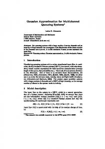
Lennard-Jones fluid with parameters ␴ = 2.749 Å, ␧ / kB = 35.6 K, and m = 3.35⫻ 10−26 kg, at a reduced density ␳* = 0.78 and temperature T* = 0.84. This state point is at a fairly low temperature, while still in the liquid region of both the Lennard-Jones and experimental phase diagrams.39,40 Quantum effects are significant under these conditions: the kinetic energy computed by path integral Monte Carlo methods is about 55.15± 0.27 K, amounting to a 20% quantum correction to the classical kinetic energy of 44.85 K. These sizable quantum mechanical effects arise from the large zero-point energy of the light neon atoms. The dynamical consequences of these quantum effects are even greater: the momentum correlation function computed by FBSD was found to differ substantially from that obtained by classical molecular dynamics methods, and various quantum correction factor prescriptions give rise to different results, none of which is in good agreement with the FBSD results.40 In this application, we used 512 000 imaginary trajectories with 20 imaginary time propagation steps, and one real time trajectory per imaginary time trajectory for the TGALSC-IVR 共10 real time trajectories per imaginary time trajectory for the TGA-FBSD兲 with 800 real time propagation steps. During the imaginary time propagation the LennardJones potential is fitted by three Gaussian functions the parameters of which are described in the literature.23 Since liquid neon is treated as an isotropic system, we choose the coherent state parameter ⌫ = ␥1, where 1 is the identity matrix and ␥ = 6, for both the PP-FBSD and the TGA-FBSD simulations. The average kinetic energy computed by the TGA methods is about 54.53± 0.07 K. Figure 4 shows the velocity correlation function for liquid neon obtained by the PP-FBSD, the TGA-LSC-IVR, and the TGA-FBSD. Both the real and imaginary parts of the correlation function are in good agreement with the PPFBSD method. The TGA-LSC-IVR correlation function 共real part兲 decays to a somewhat lower well in comparison with the TGA-FBSD and the PP-FBSD results. The comparison of

FIG. 3. 共Color online兲 As in Fig. 2, but for a much lower temperature ␤ប␻ = 8冑2. Panel 共b兲 shows a blowup of the curves shown in 共a兲.


224104-9

J. Chem. Phys. 125, 224104 共2006兲


FIG. 4. 共Color online兲 The velocity autocorrelation function of liquid neon. panel 共a兲 shows the real part of the correlation function while Panel 共b兲 depicts the imaginary part. Black solid line: PP-FBSD result. Blue solid circle with dashed line: TGA-LSC-IVR result. Red solid square with dotted line: TGA-FBSD result. Green solid line: classical result.

the semiclassical correlation function to the classical result has been shown in Fig. 4. Note that the classical correlation function has no imaginary part, i.e., it is purely real. As reported in Ref. 23, the total number of the imaginary time trajectories in the TGA can be substantially decreased if a classical distribution of q0 is generated at a reference temperature 共which can be the same temperature T = 29.90 K in this case兲, and in every thousand classical MC steps or so, choose one point q0 for the TGA imaginary time propagation, because the classical Metropolis walk is easy to achieve and thus helps the successive points q0 to sample the space efficiently. As a consequence, it should also greatly accelerate the sampling efficiency in the TGA-LSC-IVR and the TGA-FBSD. We would like to apply this technique in the future. VI. CONCLUDING REMARKS

In this paper, we have shown how the TGA can be combined with the SC-IVR to construct time correlation functions in a fully semiclassical scheme, using both real and imaginary time propagations. Specially, we have shown that both the TGA-LSC-IVR and the TGA-FBSD allow one to integrate out the oscillatory term inherent in the LSC-IVR or FBSD, and thus make them practical for descriptions of quantum dynamical effects in large molecular systems. The Kubo-transformed correlation function can also be calculated in the same fashion without additional work, as shown in Appendix B. Numerical simulations of an anharmonic oscillator and a low temperature liquid 共liquid neon兲 show that the TGALSC-IVR and the TGA-FBSD are good approximations for time correlation functions. Work is continuing to see how well they do in more challenging applications in the condensed matter phase, such as clusters23,34 and more quantum mechanical liquids 共hydrogen or helium兲. It will also be interesting in future work to see how application of the TGA can be used with a more rigorous treatment of the real time

dynamics in a SC-IVR, such as Miller’s version of the forward-backward IVR,41 or the exact forward-backward semiclassical IVR expression 共EFB-IVR兲.33 We note, however, that the TGA does not provide a good description for the Boltzmann operator in barrier problems, as is typical for the reactive flux correlation functions that determine chemical reaction rates. Current calculations, along with analytical studies 共Appendix C兲, show that the TGA fails to capture the character of the Boltzmann operator at a low temperature: at low temperature, coordinate matrix elements of the Boltzmann operator bifurcate into a dual saddle point structure described by the quantum instanton model. No Gaussian model is able to capture the nature of this bifurcation. The more rigorous imaginary time Van Vleck and the coherent state propagators in imaginary time, however, are able to describe this bifurcation semiquantitively.42 Further effort is thus being devoted to the goal of finding efficient ways of using these more rigorous SC imaginary time approximations for the Boltzmann operator within the overall SC-IVR approach to time correlation functions.

ACKNOWLEDGMENTS

This work was supported by the Office of Naval Research Grant No. N00014-05-1-0457 and by the National Science Foundation Grant No. CHE-0345280. The authors also acknowledge a generous allocation of supercomputing time from the National Energy Research Scientific Computing Center 共NERSC兲. Thanks are also due to Professor Eli Pollak for suggesting use of the TGA in SC-IVR correlation functions, and to the US Israel Binational Science Foundation for partial support of the work.


224104-10

J. Chem. Phys. 125, 224104 共2006兲


FIG. 5. 共Color online兲 Schematic representation of combined path integral LSC-IVR representation of the density 共Boltzmann operator兲 for two particles for n = 4 inserting beads. Black solid circles represent the path integral beads, red wavy lines indicate spring potentials between neighbor beads, green straight lines depict intermolecular interactions, and blue dotted lines demonstrate the connection between the end beads via the Fourier transform. The open rings illustrate the integrand in Eq. 共A2兲, while the closed ones the Wigner function of the Boltzmann operator. Note the two end beads of the open rings merge into single beads 共purple solid circles兲 at their average positions associated with the momenta coming from the Fourier transform of the difference between the two end beads, thus in this way it constructs the initial phase space in the LSC-IVR.

APPENDIX A: DIFFICULTIES IN EXACT PATH INTEGRAL REPRESENTATIONS OF THE LSC-IVR AND THE FBSD

As discussed in Sec. II, the Wigner function for operator Â␤ is nontrivial since it involves a multidimensional Fourier ˆ transform involving the Boltzmann operator e−␤H of the complete system. One way to proceed is to express the Boltzmann operator as a Feynman path integral. By inserting path integral beads 共q1 , q2 , . . . , qn兲 for the Boltzmann operator, the path integral representation of the LSC-IVR 关Eq. 共2.8兲兴 may be written as LSC-IVR 共t兲 = Z−1 CAB

冕冕冕 dp0

dq0

dq1 ¯

冕

dqn

⫻⌰共p0,q0,q1, . . . ,qn兲⌳AB共p0,q0,q1, . . . ,qn兲,

FIG. 6. 共Color online兲 Schematic representation of combined path integral FBSD representation of the density 共Boltzmann operator兲 for two particles for n = 4 inserting beads based on an early version. 共Ref. 16兲 Black solid circles represent the path integral beads, purple solid circles demonstrate the coherent state beads, red solid wavy lines indicate spring potentials between neighbor path integral beads while red dashed wavy lines illustrate the spring potential between the coherent state bead and its neighbor path integral beads, green straight lines depict intermolecular interactions, and blue dotted lines show the interaction between the two path integral beads that are neighbors to the coherent state bead from the phase term in Eq. 共A4兲. The coherent state beads are not involved in the intermolecular interaction directly in the imaginary time. Note the coherent state beads define the initial phase space in the FBSD.

where ⌬␤ = ␤ / 共n + 1兲. Figure 5 shows a schematic representation of Eq. 共A2兲. For complex systems, generally it is not possible to explicitly evaluate the Fourier transform in Eq. 共2.9兲 or 共A2兲 because of the sign problem 共the phase cancellation is severe兲. Some kinds of harmonic approximation3,6,7 for the elements of the Boltzmann operator are necessary. These approximations have been successfully applied to some complex systems.15,21 They all, however, encounter problems at low temperature when the potential energy has negative curvature; this shows up most strikingly in regions of potential barriers, but also in the long range region of bounded potentials. A similar difficulty arises in the FBSD if one uses a Feynman path integral representation of the Boltzmann operator. Introducing the path integral representation of the Boltzmann operator into Eq. 共2.15兲 yields the following form43 for the correlation function:

共A1兲 where ⌳AB共p0 , q0 , q1 , . . . , qn兲 is function related with the operators Aˆ and Bˆ, and the sampling function ⌰共p0 , q0 , q1 , . . . , qn兲 is the Fourier transform of the integrand ˆ of 具q0 − ⌬q0 / 2兩e−␤H兩q0 + ⌬q0 / 2典 after inserting the beads 共q1 , q2 , . . . , qn兲 into the elements of the Boltzmann operator, which gives ⌰共p0,q0,q1, . . . ,qn兲 = 共2␲ប兲

−3N

冕

ˆ

d⌬q0e

ipT 0 ⌬q0

具q0 − ⌬q0/2兩e ˆ

ˆ −⌬␤H

⫻具q1兩e−⌬␤H兩q2典 ¯ 具qn兩e−⌬␤H兩q0 + ⌬q0/2典,

兩q1典共A2兲

FBSD 共t兲 = 共2␲ប兲−3NZ−1 CAB

⫻

冕

冕冕冕 dp0

dq0

dq1 ¯

dqn⌰共p0,q0,q1, . . . ,qn兲

⫻⌳AB共p0,q0,q1, . . . ,qn兲,

共A3兲

where ⌳AB共p0 , q0 , q1 , . . . , qn兲 is a function related to the operators Aˆ and Bˆ, and ⌰共p0 , q0 , q1 , . . . , qn兲 is the integrand of ˆ

具q0 , p0兩e−␤H兩q0 , p0典 after inserting the beads 共q1 , q2 , . . . , qn兲 into the Boltzmann operator, which has the explicit form


224104-11

J. Chem. Phys. 125, 224104 共2006兲

Semiclassical time correlation functions ˆ

ˆ

ˆ

⌰共p0,q0,q1, . . . ,qn兲 = 具q0,p0兩e−⌬␤H0/2兩q1典e−⌬␤V共q1兲具q1兩e−⌬␤H0/2兩q2典 ¯ e−⌬␤V共qn兲具xn兩e−⌬␤H0/2兩q0,p0典

再

⬀ exp − 共q1 − q0兲TM共M + ប2⌬␤⌫兲−1⌫共q1 − q0兲 + 共qn − q0兲TM共M + ប2⌬␤⌫兲−1⌫共qn − q0兲 +

i ⌬␤ T p 共M + ប2⌬␤⌫兲−1p0 + pT0 共M + ប2⌬␤⌫兲−1M共q1 − qn兲 2 0 ប

−

1 V共qk兲 . 兺共qk − qk−1兲TM共qk − qk−1兲 − ⌬␤ 兺 2ប2⌬␤ k=2 k=1

n

冎

n

共A4兲

Usually 兩⌰共p0 , q0 , q1 , . . . , qn兲兩 would be used as the sampling function for the Monte Carlo evaluation of the integral in Eq. 共A3兲. However, the phase in Eq. 共A4兲 only vanishes when inserting one bead is sufficient for evaluating the Boltzmann operator, and thus becomes a bottleneck at low temperature for complex systems. Nakayama and Makri therefore introduced the pair-product 共PP兲 approximation so that one bead is accurate enough for low-temperature pure isotropic liquids.17 Figure 6 gives a schematic representation of Eq. 共A4兲. To summarize, for general complex systems, the rigorous path integral treatment of the Boltzmann operator in both the LSC-IVR and the FBSD methods encounters the problem—the inability to explicitly obtain the initial phase distribution for the real time trajectories—as shown in Figs. 5 and 6.

TGA-LSC-IVR and TGA-FBSD can both be expressed in a similar form as Eq. 共4.2兲 or 共4.6兲. Here we take the momentum and the force autocorrelation functions as examples. Since the momentum and force operators can be expressed as ˆ , xˆ 兴 and F共xˆ 兲 = −V⬘共xˆ 兲 = i / ប关H ˆ , pˆ 兴, their Kubo pˆ = 共i / ប兲M关H transforms are given by

APPENDIX B: TGA-LSC-IVR AND TGA-FBSD FORMULATIONS OF KUBO-TRANSFORMED CORRELATION FUNCTIONS

Equations 共B2兲 and 共B3兲 directly connect the standard real time correlation function 关Eq. 共2.1兲兴 with the Kubotransformed correlation function 关Eq. 共B1兲兴, which shows another way to calculate the Kubo-transformed correlation function. ␤ or The Wigner function and the Husimi function of pˆ Kubo ˆF␤ can be obtained analytically using the TGA in the same Kubo way as in Eqs. 共4.1兲 and 共4.5兲, respectively. The final form of the TGA-LSC-IVR of the Kubo-transformed real time correlation function can be shown to be

␤ = pˆ Kubo

i ˆ ␤ = 关pˆ ,e−␤H兴. Fˆ Kubo ប␤

共B1兲

ˆ ˆ ␤ = 1 / ␤兰0␤d␭e−共␤−␭兲HAê−␭H is the Kubowhere AˆKubo transformed operator. The Kubo-transformed versions of the

TGA-LSC-IVR CAA,Kubo 共t兲 =

1 Z

冕

dq0

1 exp共2␥共␤/2兲兲共4␲兲3N/2 兩det G共␤/2兲兩1/2

⫻exp − pT0 G

冉

TGA-LSC-IVR x0,p0,q f AA,Kubo

dx0

冉冊冊

␤ 2

T

G−1

␤ 2

x0 − q

␤ 2

dp0

兩det G共␤/2兲兩1/2 共␲ប2兲3N/2

␤ ␤ TGA-LSC-IVR p0/ប2 f AA,Kubo ;t , x0,p0,q 2 2

冉冊

2 ␤ ␤ ;t = 2 pT0 MG pt 2 ប␤ 2

共B3兲

1 ␲3N/2兩det G共␤/2兲兩1/2

冉冉冉冊冊冉冊冉冉冊冊冊冕冉冉冊冊冉冉冊冊

⫻exp − x0 − q

where

冕

共B2兲

and

The Kubo-transformed real time correlation function44 is given as 1 ˆ ˆ Kubo ␤ CAB 共t兲 = Tr共AˆKubo eiHt/បBê−iHt/ប兲, Z

i ˆ M关xˆ ,e−␤H兴 ប␤

共B4兲

共B5兲

for the momentum Aˆ = pˆ , and Downloaded 14 Mar 2008 to 136.152.154.126. Redistribution subject to AIP license or copyright; see http://jcp.aip.org/jcp/copyright.jsp

224104-12

冉

冉冊冊冉冉冊冊冉冊

TGA-LSC-IVR f AA,Kubo x0,p0,q

=−

J. Chem. Phys. 125, 224104 共2006兲


␤ ;t 2

2 ␤ x0 − q ␤ 2

T

G−n

␤ Ft共x0,p0兲 2

共B6兲

for the force Aˆ = Fˆ . TGA-LSC-IVR TGA-LSC-IVR The formula of CAA,Kubo 共t兲 and that of CAA 共t兲 in Eq. 共4.2兲 show that they share exactly the same MC TGA-LSC-IVR TGA-LSC-IVR sampling, except that the estimator function f AA,Kubo 共x0 , p0 , q共␤ / 2兲 ; t兲 is different from f AA 共x0 , p0 , q共␤ / 2兲 ; t兲, so they are able to be calculated simultaneously. Similarly, we obtain the following result for the TGA-FBSD version of the Kubo-transformed correlation function: TGA-FBSD 共t兲 = CAA,Kubo

1 Z ⫻ ⫻

where

冕冕冕

冉

TGA-FBSD f AA,Kubo x0,p0,q

dq0

1 exp共2␥共␤/2兲兲共4␲兲3N/2 兩det G共␤/2兲兩1/2

dx0

兩det ⌫兩1/2 exp共− 共x0 − q共␤/2兲兲TG−1共␤/2兲共⌫ + 共1/2兲G−1共␤/2兲兲−1⌫共x0 − q共␤/2兲兲兲 ␲3N/2兩det G共␤/2兲兩1/2兩det共⌫ + 共1/2兲G−1共␤/2兲兲兩1/2

dp0

exp共− pT0 共⌫ + 共1/2兲G−1共␤/2兲兲−1p0/2ប2兲 TGA-FBSD ␤ x0,p0,q ;t , 2 3N/2 −1 1/2 f AA,Kubo 共2␲ប 兲兩det共⌫ + 共1/2兲G 共␤/2兲兲兩 2

冉

冉冊冊

共B7兲

冉冊冊冋冉冊冉冉冊冊冉冉冊冊冉冉冊冊冉冊冉冉冊冊冉冉冊冊冉冊冉冉冊冊册冉冉冉冊冊冊冉冉冊冊冉冉冊冊 ␤ ;t = 2

1+

3N 1 1 ␤ − 2 pT0 ⌫ + G−1 2 2 2ប 2

1 ␤ ⫻ ⌫ + G−1 2 2 ⫻

−1

−1

1 ␤ ⌫ ⌫ + G−1 2 2

1 −1 ␤ 1 T 2 pt M ⌫ + G 2 ប␤ 2

1 ␤ ⌫ ⌫ + G−1 2 2 −1

G−1

␤ 2

−1

p0 −

x0 − q

p0 +

T

G−1

␤ 2

␤ 2

1 T 1 −1 ␤ 2 pt M ⌫ + G 2 ប␤ 2

−1

1 ␤ x0 − q 2 2

−1

1 ␤ ⌫ ⌫ + G−1 2 2

−1

p0

共B8兲 for the momentum Aˆ = pˆ , and

冉

TGA-FBSD f AA,Kubo x0,p0,q

冉冊冊冋冉冊冉冉冊冊冉冉冊冊冉冉冊冊冉冊冉冉冊冊冉冉冊冊冉冊冉冉冊冊册冉冉冉冊冊冉冉冊冊冉冊冊冉冉冊冊冉冊冉冉冊冊冉冉冊冊冉冊 ␤ ;t = 2

1+

3N 1 1 ␤ − 2 pT0 ⌫ + G−1 2 2 2ប 2

1 ␤ ⫻ ⌫ + G−1 2 2 ⫻ −

2 ␤ x0 − q ␤ 2

1 ␤ ⫻ ⌫ + G−1 2 2

−1

1 ␤ ⌫ ⌫ + G−1 2 2

T

−1

−1

1 ␤ ⌫ ⌫ + G−1 2 2

1 ␤ ⌫ ⌫ + G−1 2 2

for the force Aˆ = Fˆ .

1 ␤ ⌫ ⌫ + G−1 2 2 −1

G−1

It can be shown that the matrix G共␶兲 in Eq. 共3.2兲 is always positive definite for a physical system 共for which the second derivative of the potential is zero or positive in the asymptotic region兲. Therefore, since matrix elements of the Boltzmann operator are given within the TGA by

p0 −

x0 − q

1 ␤ x0 − q 2 2

1 ␤ ␤ Ft − x0 − q 2 ␤ 2

G−1

␤ Ft 2

−1

T

G−1

␤ 2

␤ 2

G−1

−1

T

G−1

␤ 2

共B9兲

ˆ

具x − ⌬x/2兩e−␤H兩x + ⌬x/2典 =

APPENDIX C: PROBLEM OF TGA TREATMENT OF THE BOLTZMANN OPERATOR OF THE BARRIER POTENTIAL

␤ 2

−1

=

冕冕冉冊

ˆ

ˆ

dq0具x − ⌬x/2兩e−␤H/2兩q0典具q0兩e−␤H/2兩x + ⌬x/2典 dq0

冉

1 2␲

3N

exp共2␥共␤/2兲兲兩det G共␤/2兲兩

1 ⫻exp − ⌬xTG−1共␤/2兲⌬x 4

冊

⫻exp共− 共x − q共␤/2兲兲TG−1共␤/2兲共x − q共␤/2兲兲兲, 共C1兲


224104-13

and since G共␤ / 2兲 is positive definite, the matrix element along the off-diagonal direction ⌬x is always a Gaussian centered at 0. This is qualitatively wrong, however, for a barrier potential 共i.e., Eckart barrier兲 at low temperature, ˆ where the element 具−⌬x / 2兩e−␤H兩⌬x / 2典 is typically bimodal; i.e., the TGA is intrinsically incapable of capturing the two saddle points 共along the off-diagonal direction ⌬x兲 of the coordinate Boltzmann matrix element for a barrier potential, which is characteristic of the low temperature regime, as shown in Fig. 1共a兲 in Ref. 45. This bimodal character, however, is described semiquantitively by the more rigorous imaginary time Van Vleck and the Herman-Kluk propagators in imaginary times.42 J. Cao and G. A. Voth, J. Chem. Phys. 100, 5106 共1994兲; S. Jang and G. A. Voth, ibid. 111, 2371 共1999兲; I. R. Craig and D. E. Manolopoulos, ibid. 121, 3368 共2004兲. 2 X. Sun, H. B. Wang, and W. H. Miller, J. Chem. Phys. 109, 4190 共1998兲. 3 H. B. Wang, X. Sun, and W. H. Miller, J. Chem. Phys. 108, 9726 共1998兲. 4 J. Shao and N. Makri, J. Phys. Chem. A 103, 7753 共1999兲. 5 J. Shao and N. Makri, J. Phys. Chem. A 103, 9479 共1999兲. 6 J. A. Poulsen, G. Nyman, and P. J. Rossky, J. Chem. Phys. 119, 12179 共2003兲. 7 Q. Shi and E. Geva, J. Phys. Chem. A 107, 9059 共2003兲. 8 J. H. Van Vleck, Proc. Natl. Acad. Sci. U.S.A. 14, 178 共1928兲; M. C. Gutzwiller, Chaos In Classical and Quantum Mechanics 共Springer, New York, 1990兲. 9 W. H. Miller, J. Chem. Phys. 53, 3578 共1970兲. 10 W. H. Miller, J. Phys. Chem. A 105, 2942 共2001兲. 11 W. H. Miller, J. Chem. Phys. 95, 9428 共1991兲; E. J. Heller, ibid. 95, 9431 共1991兲; 94, 2723 共1991兲; K. G. Kay, ibid. 100, 4377 共1994兲; 100, 4432 共1994兲. 12 M. F. Herman and E. Kluk, Chem. Phys. 91, 27 共1984兲. 13 R. Gelabert, X. Gimenez, M. Thoss, H. B. Wang, and W. H. Miller, J. Chem. Phys. 114, 2572 共2001兲; X. Sun, H. B. Wang, and W. H. Miller, ibid. 109, 7064 共1998兲; H. Wang, X. Song, D. Chandler, and W. H. Miller, ibid. 110, 4828 共1999兲; H. Wang, M. Thoss, K. L. Sorge, R. Gelabert, X. Gimenez, and W. H. Miller, ibid. 114, 2562 共2001兲; M. L. Brewer, J. S. Hulme, and D. E. Manolopoulos, ibid. 106, 4832 共1997兲; F. Grossmann, Phys. Rev. A 60, 1791 共1999兲; N. J. Wright and N. Makri, J. Phys. Chem. B 108, 6816 共2004兲; A. Nakayama and N. Makri, Proc. Natl. Acad. Sci. U.S.A. 102, 4230 共2005兲. 14 X. Sun and W. H. Miller, Abstr. Pap. - Am. Chem. Soc. 213, 94 共1997兲. 15 J. A. Poulsen, G. Nyman, and P. J. Rossky, J. Phys. Chem. B 108, 19799 共2004兲. 16 N. J. Wright and N. Makri, J. Chem. Phys. 119, 1634 共2003兲. 1

J. Chem. Phys. 125, 224104 共2006兲


A. Nakayama and N. Makri, J. Chem. Phys. 119, 8592 共2003兲. J. Liu, A. Nakayama, and N. Makri, Mol. Phys. 104, 1267 共2006兲. 19 A. R. Walton and D. E. Manolopoulos, Mol. Phys. 87, 961 共1996兲; H. B. Wang, D. E. Manolopoulos, and W. H. Miller, J. Chem. Phys. 115, 6317 共2001兲; X. Sun and W. H. Miller, ibid. 110, 6635 共1999兲; K. Thompson and N. Makri, Phys. Rev. E 59, R4729 共1999兲; J. Chem. Phys. 110, 1343 共1999兲. 20 N. Makri and K. Thompson, Chem. Phys. Lett. 291, 101 共1998兲. 21 Q. Shi and E. Geva, J. Phys. Chem. A 107, 9070 共2003兲. 22 S. Bonella, D. Montemayor, and D. F. Coker, Proc. Natl. Acad. Sci. U.S.A. 102, 6715 共2005兲. 23 P. A. Frantsuzov and V. A. Mandelshtam, J. Chem. Phys. 121, 9247 共2004兲. 24 P. Frantsuzov, A. Neumaier, and V. A. Mandelshtam, Chem. Phys. Lett. 381, 117 共2003兲. 25 E. J. Heller, Chem. Phys. Lett. 34, 321 共1975兲; E. J. Heller, J. Chem. Phys. 64, 63 共1976兲. 26 B. Hellsing, S. I. Sawada, and H. Metiu, Chem. Phys. Lett. 122, 303 共1985兲. 27 J. Shao and E. Pollak, J. Chem. Phys. 125, 133502 共2006兲. 28 N. Makri and W. H. Miller, J. Chem. Phys. 116, 9207 共2002兲. 29 Y. Zhao and W. H. Miller, J. Chem. Phys. 117, 9605 共2002兲. 30 B. J. Berne and G. D. Harp, Adv. Chem. Phys. 17, 63 共1970兲. 31 W. H. Miller, S. D. Schwartz, and J. W. Tromp, J. Chem. Phys. 79, 4889 共1983兲. 32 W. H. Miller, Adv. Chem. Phys. 25, 69 共1974兲; Proc. Natl. Acad. Sci. U.S.A. 102, 6660 共2005兲. 33 W. H. Miller, J. Chem. Phys. 125, 132305 共2006兲. 34 P. A. Frantsuzov, D. Meluzzi, and V. A. Mandelshtam, Phys. Rev. Lett. 96, 113401 共2006兲; P. A. Frantsuzov and V. A. Mandelshtam, Phys. Rev. E 72, 037102 共2005兲. 35 D. C. Marinica, M. P. Gaigeot, and D. Borgis, Chem. Phys. Lett. 423, 390 共2006兲. 36 E. Jezek and N. Makri, J. Phys. Chem. 105, 2851 共2001兲; M. Thoss, H. B. Wang, and W. H. Miller, J. Chem. Phys. 114, 9220 共2001兲. 37 K. Thompson and N. Makri, Phys. Rev. E 59, R4729 共1999兲. 38 J. Liu and N. Makri, Chem. Phys. 322, 23 共2006兲. 39 Thermodynamic Properties of Neon, Argon, Krypton, and Xenon, edited by V. A. Rabinovich, A. A. Vasserman, V. I. Nedostup, and L. S. Veksler 共Springer-Verlag, Berlin, 1988兲; J. K. Johnson, J. A. Zollweg, and K. E. Gubbins, Mol. Phys. 78, 591 共1993兲. 40 C. P. Lawrence, A. Nakayama, N. Makri, and J. L. Skinner, J. Chem. Phys. 120, 6621 共2004兲. 41 W. H. Miller, Faraday Discuss. 110, 1 共1998兲. 42 C. Venkataraman 共private communication兲. 43 N. Makri, J. Phys. Chem. B 106, 8390 共2002兲. 44 R. Kubo, M. Toda, and N. Hashitsume, Statistical Physics, 2nd ed. 共Springer-Verlag, Heidelberg, 1991兲. 45 W. H. Miller, Y. Zhao, M. Ceotto, and S. Yang, J. Chem. Phys. 119, 1329 共2003兲. 17 18
