Index TermsâUltrasound imaging, sparse regularization. I. INTRODUCTION ... fluctuations in acoustic velocity and/or density, defining a tissue reflectivity ... In this setting, the pulse-echo spatial impulse response model [9], [10] ..... [10] P. R. Stepanishen, âThe timeâdependent force and radiation impedance on a piston in a ...
USSR: An UltraSound Sparse Regularization Framework Adrien Besson∗ , Dimitris Perdios∗ , Florian Martinez∗ , Marcel Arditi∗ , Yves Wiaux† , and Jean-Philippe Thiran∗‡
∗ Signal
Processing Laboratory (LTS5), Ecole Polytechnique Fédérale de Lausanne, Lausanne, Switzerland † Institute of Sensors, Signals and Systems, Heriot-Watt University, Edinburgh, UK ‡ Department of Radiology, University Hospital Center (CHUV) and University of Lausanne (UNIL), Lausanne, Switzerland
II. USSR: U LTRA S OUND S PARSE R EGULARIZATION FRAMEWORK
m pi , tl
�
A. The matrix-free measurement model operator
“wavefront”
t pi
n)
, pi �
x
t T x (r
Ultrafast ultrasound (US) imaging exploits the idea of using plane waves (PW) or diverging waves (DW) to insonify the whole field-of-view at once, allowing US systems to reach, in theory, thousands of frames per second. One main limitation of ultrafast US imaging is a degraded image quality, compared to classical US imaging where multiple focused beams are used on transmit. One way to address such a problem is coherent compounding [1] where images obtained with different insonification angles are averaged. While the implementation of such a technique is straightforward, it requires multiple insonifications thus reducing the frame rate. An alternative to compounding consists in using more efficient reconstruction methods than classical techniques, which revolve around delay-and-sum (DAS) beamforming. One popular group of methods relies on the use of iterative algorithms to solve the ill-posed problem induced by US image reconstruction. These methods are built upon forward models of the problem. David et al. [2] and Besson et al. [3] have proposed time-domain formulations of the problem. Besson et al. have presented a forward model in the Fourier domain in which US propagation is seen as a projection on a non-uniform Fourier space [4]. Schiffner and Schmitz have proposed a timefrequency model in which each frequency of the transducerelement bandwidth is treated independently [5]. These methods are computationally complex which severely limits their appeal against analytical ones. In this paper, we introduce USSR, an UltraSound Sparse Regularization framework, composed of two main components. First, highly parallelizable parametric and matrix-free formulations of a time-domain measurement model and its
rn
I. I NTRODUCTION
adjoint are introduced in the context of PW imaging. Secondly, the proposed formulations are involved in a sparse regularization algorithm, where two different sparsity priors, namely the `1 -norm in a sparsity averaging (SA) model [4], and the `p norm in the image domain [6], are suggested. The framework is implemented on multi-thread architectures which permit high-quality reconstructions two to three orders of magnitude faster than state-of-the art approaches. The remainder of the paper is organized as follows. In Section II, USSR is introduced and its implementation is detailed. In Section III, several applications of USSR are described and the high-quality reconstruction is demonstrated on the PICMUS dataset [7]. Concluding remarks are given in Section IV.
tRx
Abstract—Ultrafast ultrasound (US) imaging uses unfocused waves to insonify the whole medium of interest at once, allowing pulse-echo US imaging to achieve very high frame rates, at the cost of a lower image quality. In this paper, we present USSR, an UltraSound Sparse Regularization framework which permits high-quality imaging at fast rates and with a very low memory footprint. The framework, based on highly parallelizable, parametric, matrix-free formulations of the measurement model and its adjoint as well as on well-chosen sparsity priors, is implemented on multi-threaded architectures and evaluated on the publicly available PICMUS dataset. Index Terms—Ultrasound imaging, sparse regularization
(r n , γ (r n )) z Fig. 1: Standard 2D ultrafast US imaging configuration. Ultrafast US imaging involves the transmission of PWs or DWs on the insonified medium. In such a setting, it is known that the image reconstruction can be expressed as an inverse problem [5], [2]. More precisely, let us consider the pulseecho experiment described on Figure 1, where the propagation
medium Ω ∈ R2 \ {z ≤ 0} contains inhomogeneities as local fluctuations in acoustic velocity and/or density, defining a tissue reflectivity function (TRF) γ (r) with r ∈ Ω [5], [8]. The medium is insonified with a 1D-array of Nel transducer elements, located at pi ∈ Π, where i ∈ {1, ..., Nel } and the echo signals detected by the same elements are denoted as � m pi , tl , where tl = t0 + l∆t, with l ∈ {1, ..., Nt }. We choose to discretize the insonified medium with the following grid: r n = [xk , z l ]T , (k, l) ∈ {1, .., Nx }×{1, .., Nz } and n = (k − 1)Nz + l. We also introduce the two following ��Nt Nz Nx and m = m pi , tl pi ∈Π,l=1 . vectors γ = (γ (r n ))n=1 In this setting, the pulse-echo spatial impulse response model [9], [10] can be written as: Z � � i l m p ,t = od r, pi γ (r) r∈Ω
vpe tl − tT x (r) − tRx r, pi
��
dr,
(1)
where vpe (t) denotes the pulse-echo waveform, t T x (r) is
the � propagation delay on transmit, tRx r, pi = r − pi� 2 /c i is the �propagation =
delay on receive� and od r, p
o r, pi /2π r − pi 2 where o r, pi accounts for the element directivity [11]. The model described in Equation (1) can be rewritten as: � ZZ � od r, pi γ (r) i l dσ (r) m p ,t = | ∇r g |
˜ pi where ∗t��denotes the 1D-convolution and m i l m ˜ p , t tl ∈T defined by:
vpe tl − τ dτ, (2) � � � where g r, pi , t = t − tT x (r) − tRx r, pi , Γ pi , t = � � r ∈ Ω | g r, pi , t = 0 , ∇r g denotes the gradient of g with respect to the�variable r, dσ (r) is the measure over the 1Dcurve Γ pi , t . In the light of Equation (2), the measurements are obtained by projecting� the reflectivity values onto the 1Dcurve defined by Γ pi , t and by convolving the results with the pulse shape. In order to have an efficient way of calculating the integral defined � in Equation (2), we derive a parameterization of Γ pi , t as follows: � � � ��T T r = [x, z] ∈ Γ pi , t ⇔ r α, pi , t = α, f α, pi , t , (3) where α ∈ R, which allows us to rewrite Equation (2) as: ZZ � � � �� m pi , tl = od r α, pi , tl , pi γ r α, pi , tl τ ∈R,α∈R
� | Jα | dαvpe tl − τ dτ, (4) | ∇r g | where |Jα | is the Jacobian associated with the change of variable. Thanks to the reparameterization of the integral, the discretization can be easily achieved as: � � � � ˜ pi ∗t vpe tl , (5) m pi , tl = m
=
d
Nx � X � � wk od r αk , pi , tl , pi m ˜ pi , tl = k=1
ϕ r αk , pi , tl
��
γ, (6)
where wk is the integration weight multiplied by the terms related to the change of variable and ϕ is a 1D-interpolation kernel. Finally, one can write the measurement model associated with the pulse-echo experiment for each point of the measurement grid as: � � m pi , tl = Hd {γ} pi , tl , (7) � � � l� i l i ˜ p ∗t vpe t is a linear where Hd {γ} p , t = m operator. B. Set of parametric equations for plane wave imaging The equivalence (3) defines a set of parametric equations which depends on the transmit delay. When a steered PW, with angle θ is transmitted in the medium, the propagation delay on transmit can be written as tT x (r) =< r, kθ > /c, where T kθ = [cos (θ) , sin (θ)] . In this case, the set of parametric equations is obtained by finding the roots of the function: q 2 2 f (z) = (x − pix ) + (z − piz ) + z cos (θ) + x sin (θ) − ct, (8)
τ ∈R,r∈Γ(pi ,τ )
�
�
which gives the following solution: � √ � 1 i z= ∆ , 2 pz − ct cos (θ) + x sin (θ) cos (θ) ± sin (θ) (9) where ∆ = ct − piz cos (θ) − pix sin (θ)
�
� � × ct − piz cos (θ) + pix − 2x sin (θ) . (10) C. The matrix-free adjoint operator of the measurement model The adjoint operator of the linear operator Hd {γ} defined in Equation (7) is defined, in the continuous domain, as: X � H† {m} (r n ) = od r n , pi pi ∈Π
Z
� � m pi , τ u tT x (r n ) + tRx r n , pi − τ dτ, (11) �
τ ∈R
where u (t) = vpe (−t) is the matched filter of the pulse shape. The discretization of the adjoint operator described in Equation (11) leads to: X � Hd† {m} (r n ) = ω n od r n , pi pi ∈Π
ψ tT x (r n ) + tRx r n , pi
��
ˆ m, (12)
ˆ = m ∗t u, ψ is a 1D-interpolation kernel and ω n where m accounts for the integration weight.
D. The image reconstruction procedure The linear measurement operator Hd {γ} described in Section II-A defines an ill-posed linear inverse problem which can be equivalently written as [12]: m = Hd γ + ν,
γ∈RNx Nz
λR (γ) +
1 2 kHd γ − mk2 , 2
III. A PPLICATIONS OF USSR
(13)
where Hd ∈ RNel Nt ×Nx Nz is the matrix associated with the linear measurement model and ν ∈ RNel Nt is the noise due to the model discrepancy and the discretization. To solve this problem, we use a sparse regularization framework which solves the following optimization problem: min
model and the adjoint, in order to compute the derivative of the data-discrepancy term. Two implementations of the framework are proposed, one using CUDA for NVIDIA GPU platforms and one using OpenMP for CPU platforms1 .
(14)
where R (γ) accounts for the prior term and λ ∈ R+ is the regularization parameter. The image reconstruction procedure proposed in (14) is rather general and may be compatible with any convex functional R (γ). In this work, we have focused on two priors that have been successfully used in US imaging: p • The `p -norm to the power of p: R (γ) = kγkp , p ≥ 1;
† • The `1 -norm in the SA model: R (γ) = Ψ γ , 1 where Ψ = √1q [Ψ1 , ..., Ψq ], with Ψi the i-th Daubechies wavelet. E. Implementation of USSR The main advantage of the measurement model described in Section II-A resides in the fact that it is highly parallelizable, therefore particularly suited for multi-thread architectures. Indeed, the operation Hd γ can be achieved in parallel, for each point of the element raw-data grid, following the steps below: For each transducer element pi ∈ Π: 1) For each time instant tl : a) For each point αk = xk of the image grid: � i) Compute r αk , pi , tl ; � � ii) Compute od r αk , pi , tl��, pi and wk ; iii) Compute ϕ r αk , pi , tl γ; � iv) Compute the value to sum to m ˜ pi , tl according to Equation (6); � � � � ˜ pi ∗t vpe tl according 2) Compute m pi , tl = m to Equation (5). A very similar procedure may be achieved to compute the adjoint operator of the measurement model: ˆ = m ∗t u; 1) Compute m 2) For each point of the image grid r n : a) For each transducer element pi : � i) Compute od r n , pi and ω n ; �� ˆ ii) Compute ψ tT x (r n ) + tRx r n , pi m; iii) Compute the value to sum to Hd† {m} (r n ) according to Equation (12). Regarding the optimization algorithm, Problem (14) is solved using the fast iterative shrinkage algorithm (FISTA) [13] in which each step involves the evaluation of the measurement
A. Experimental settings The proposed framework is tested on the numerical phantom and the in-vivo carotid of the PICMUS dataset2 [7] for 1 PW transmission. The quality metrics of interest are the contrastto-noise ratio (CNR) computed on the anechoic cyst of the numerical phantom vs. echo levels in adjacent “tissue", and the lateral and axial resolutions, computed as the average of the full width at half maximum of the 10 points located at 14 mm depth and 45 mm depth, respectively. Two sparse reconstruction methods are evaluated with a sparsity prior in the SA model (decomposition level 1) and with a `p -norm prior as described in Section II-A. The DAS algorithm, evaluated as a reference, is computed using a spline interpolation for the delay calculation and a receive apodization based on the element-directivity is used on receive [11]. In both cases, 200 iterations of FISTA are performed, and µ is empirically tuned. B. Results TABLE I C ONTRAST AND RESOLUTION OF THE METHODS ON THE NUMERICAL PHANTOM . CNR [dB] DAS - 1 PW DAS - 5 PWs USSR - `p USSR - SA
8.0 13.5 7.1 10.3
Lat. res. [mm] 14 mm 45 mm 0.38 0.55 0.38 0.55 0.23 0.31 0.24 0.31
Ax. res. [mm] 14 mm 45 mm 0.39 0.42 0.39 0.42 0.20 0.23 0.16 0.19
The CNR, axial and lateral resolution computed on the numerical phantom, summarized in Table I, show that both reconstruction methods recover high resolution images. Regarding the contrast, the method coupled with SA has a higher CNR than DAS with 1 PW insonification but significantly lower than DAS with 5 PW insonifications, due to the decrease of speckle density induced by the higher resolution. Visual assessment of the recovered B-mode images, displayed on Figure 2 confirms the results obtained with the metrics. Regarding the in-vivo carotids, the proposed methods lead to significantly higher quality images than the ones obtained with the DAS algorithm. Regarding the timings, 200 iterations of FISTA take around 4.5 s with the current implementation (not optimized) on an NVIDIA GeForce GTX 1080 Ti GPU, for both the `p -norm and the SA model. This can be explained by the fact that most of the time is spent computing the measurement model and the adjoint operator. We believe that a substantial gain may be achieved by optimizing the code. 1 Code
available at https://github.com/LTS5/USSR-IUS2017
2 https://www.creatis.insa-lyon.fr/EvaluationPlatform/picmus/index.html
-30 dB
30 -40 dB
40
-10 dB -20 dB
20
-30 dB
30 -40 dB
40
-50 dB -60 dB
0
-10
0
-40 dB
-30 dB
30 -40 dB
40
-50 dB
-20 dB
20
-30 dB
30 -40 dB
40
-50 dB
-60 dB
0
0
10
Lateral dimension [mm]
(e)
-50 dB -60 dB
10
-10
(f)
0
10
Lateral dimension [mm]
(d) 0 dB
10
0 dB
10
-10 dB -20 dB
20
-30 dB
30 -40 dB
40
-50 dB
-60 dB
-10
-40 dB
-60 dB
-10
-10 dB
10
Lateral dimension [mm]
-30 dB
30
(c)
10
Depth [mm]
-20 dB
20
-20 dB
20
Lateral dimension [mm] 0 dB
-10 dB
-10 dB
40
-50 dB
(b)
10
Depth [mm]
30
10
0 dB
0
-30 dB
Lateral dimension [mm]
(a)
-10
-20 dB
20
-60 dB
10
Lateral dimension [mm]
Depth [mm]
-10
-10 dB
40
-50 dB
0 dB
10
Depth [mm]
-20 dB
20
0 dB
10
Depth [mm]
-10 dB
Depth [mm]
Depth [mm]
0 dB
10
Depth [mm]
0 dB
10
-10 dB -20 dB
20
-30 dB
30 -40 dB
40
-50 dB
-60 dB
-10
0
10
Lateral dimension [mm]
(g)
-60 dB
-10
0
10
Lateral dimension [mm]
(h)
Fig. 2: Image of the numerical phantom reconstructed with (a) DAS - 1 PW insonification, (b) DAS - 5 PW insonifications, (c) USSR-SA - 1 PW insonification, (c) USSR - `p - 1 PW insonification; Image of the in-vivo carotid reconstructed with (e) DAS - 1 PW insonification, (f) DAS - 5 PW insonifications, (g) USSR-SA - 1 PW insonification, (h) USSR-`p - 1 PW insonification.
IV. C ONCLUSION We propose USSR, an UltraSound Sparse Regularization framework based on sparse regularization, as an alternative to DAS imaging. We describe matrix-free formulations of the measurement model and its adjoint in the context of PW imaging, which allow us to provide fast reconstructions with a low memory footprint. The framework is equipped with two models for the priors, namely `p -norm prior in the image domain and `1 -norm prior prior in a sparsity averaging model. The evaluation is performed on the publicly available PICMUS dataset, so that the results presented in this work are reproducible, and show that the proposed method yields improved image quality compared to state-of-the art methods. ACKNOWLEDGEMENTS This work was supported in part by the UltrasoundToGo RTD project (no. 20NA21_145911), evaluated by the Swiss NSF and funded by Nano-Tera.ch with Swiss Confederation financing. R EFERENCES [1] G. Montaldo, M. Tanter, J. Bercoff, N. Benech, and M. Fink, “Coherent plane-wave compounding for very high frame rate ultrasonography and transient elastography,” IEEE Trans. Ultrason. Ferroelectr. Freq. Control, vol. 56, no. 3, pp. 489–506, 2009. [2] G. David, J.-L. Robert, B. Zhang, and A. F. Laine, “Time domain compressive beam forming of ultrasound signals,” J. Acoust. Soc. Am., vol. 137, no. 5, pp. 2773–2784, 2015. [3] A. Besson, R. E. Carrillo, O. Bernard, Y. Wiaux, and J.-P. Thiran, “Compressed delay-and-sum beamforming for ultrafast ultrasound imaging,” in IEEE Int. Conf. Image Process., 2016, pp. 2509–2513.
[4] A. Besson, M. Zhang, F. Varray, H. Liebgott, D. Friboulet, Y. Wiaux, J.-P. Thiran, R. E. Carrillo, and O. Bernard, “A sparse reconstruction framework for Fourier-based plane-wave imaging,” IEEE Trans. Ultrason. Ferroelectr. Freq. Control, vol. 63, no. 12, pp. 2092–2106, 2016. [5] M. F. Schiffner and G. Schmitz, “Fast pulse-echo ultrasound imaging employing compressive sensing,” IEEE Int. Ultrason. Symp., 2011. [6] Z. Chen, A. Basarab, and D. Kouamé, “Compressive deconvolution in medical ultrasound imaging,” IEEE Trans. Med. Imaging, vol. 35, no. 3, pp. 728–737, 2016. [7] H. Liebgott, A. Rodriguez-Molares, F. Cervenansky, J. Jensen, and O. Bernard, “Plane-wave imaging challenge in medical ultrasound,” in IEEE Int. Ultrason. Symp., 2016. [8] O. Michailovich and D. Adam, “A novel approach to the 2-D blind deconvolution problem in medical ultrasound,” IEEE Trans. Med. Imaging, vol. 24, no. 1, pp. 86–104, 2005. [9] G. E. Tupholme, “Generation of acoustic pulses by baffled plane pistons,” Mathematika, vol. 16, no. 02, p. 209, 1969. [10] P. R. Stepanishen, “The time–dependent force and radiation impedance on a piston in a rigid infinite planar baffle,” J. Acoust. Soc. Am., vol. 49, no. 3B, pp. 841–849, 1971. [11] A. R. Selfridge, G. S. Kino, and B. T. Khuri-Yakub, “A theory for the radiation pattern of a narrow-strip acoustic transducer,” Appl. Phys. Lett., vol. 37, no. 1, p. 35, 1980. [12] A. G. J. Besson, D. Perdios, F. Martinez, Z. Chen, R. E. Carrillo, M. Arditi, Y. Wiaux, and J.-P. Thiran, “Ultrafast ultrasound imaging as an inverse problem: Fast and matrix-free measurement model for sparsity-driven image reconstruction methods,” EPFL, Tech. Rep. EPFLARTICLE-226198, 2017. [13] A. Beck and M. Teboulle, “A fast iterative shrinkage-thresholding algorithm for linear inverse problems,” SIAM J. Imaging Sci., vol. 2, no. 1, pp. 183–202, 2009.