... using cache, and maximizing algorithm simplicity to implement powerful ...... Solver Paradigm with Adaptive Cartesian Grids,â AIAA-2008-7117, 26th AIAA ...
AIAA 2009-3792
19th AIAA Computational Fluid Dynamics 22 - 25 June 2009, San Antonio, Texas
Validation of the Strand Grid Approach Andrew M. Wissink∗ US Army Aeroflightdynamics Directorate, Moffett Field, CA 94035-1000
Aaron J. Katz† Stanford University, Stanford, CA 94305
William M. Chan‡ NASA Ames Research Center, Moffett Field, CA 94035-1000
Robert L. Meakin§ University of Alabama, Birmingham, AL 35294-1150 We explore a new approach for automated mesh generation for viscous flows around geometrically complex bodies. A prismatic-like grid using “strands” is grown a short distance from the body surface to capture the viscous boundary layer, and adaptive Cartesian grids are used throughout the rest of the domain. The advantages of this approach are many; nearly automatic grid generation from triangular or quadrilateral surface tessellations, very low memory overhead, and automatic mesh adaptivity for time-dependent problems, and fast and efficient solvers from structured data in both the strand and Cartesian grids. Solvers on the two grid systems are coupled using a Chimera overset approach so the scheme is readily applicable to problems with moving bodies. The paper focuses on validation of the approach for fundamental flow problems, fixed-wing, and rotary-wing applications. Comparison to experiment and to other well-established codes are provided. Results show the approach shows considerable promise, with load computations from the automatically generated strand meshes comparable in accuracy to manually generated fully unstructured meshes, and with excellent resolution of vortex wakes.
I.
Introduction
It is well known from a long history of aerospace vehicle design that identification of potential design flaws early in the design cycle can lead to much greater cost savings, in both time and money, than taking corrective action later once the design has been established. Although computational fluid dynamics (CFD) offers the ability to perform high-fidelity predictions of vehicle performance at relatively low cost, and hence identify design issues early, its application is still quite limited in early design studies, at least compared to lower-fidelity empirically-based codes. Computational cost is often cited as the reason CFD is not more widely used. However, a comparison of the average speed of the top 500 high performance computing (HPC) systems today shows that parallel execution rate has increased approximately 1000X over the past decade. If computational cost were indeed the limiting factor, why hasn’t this huge increase in available computing power translated into more widespread use of CFD? One reason could be that computational cost is actually not the critical limiting factor. The complexity of CFD processes, in particular geometry manipulation and mesh generation, which today remain tedious and manual processes, may be the critical element preventing more widespread use of CFD in early design analysis. In spite of the variety of commercial unstructured mesh generation tools available, it is still common for an expert analyst to spend multiple days to weeks building the mesh system of a geometrically complex ∗ Senior
Research Scientist, Scaled Numerical Physics LLC, MS 215-1, AIAA Member Student, Dept. Aeronautical Engineering, AIAA Member ‡ Computer Scientist, Applications Branch, NAS Division, MS T27B-1, AIAA Senior Member § Professor, Dept. Mechanical Engineering, AIAA Fellow † Graduate
1 of 21 American Institute of Aeronautics and Astronautics Copyright © 2009 by the American Institute of Aeronautics and Astronautics, Inc. The U.S. Government has a royalty-free license to exercise all rights under the copyright claimed herein for Governmental purposes. All other rights are reserved by the copyright owner.
3D configuration before even beginning the flow solution. The computational approach described in this work seeks to automate this process by skipping the manual unstructured mesh generation process entirely, automatically building a viscous-quality prismatic mesh directly from a surface tessellation. The surface can include triangles, quadrilaterals, or any other representation. One time consuming step this work does not address is dealing with gaps in poor-quality CAD models which often cause difficulties in generating the surface mesh. However, this is typically a problem with older CAD models of legacy vehicles, i.e. those already in the fleet. With new designs generated from CAD packages that utilize solid geometries, a geometric surface tessellation can be built almost automatically. After applying some massaging of the geometric tessellation - appropriate grid spacing, enforcing smoothly varying point redistribution, clustering around sharp corners, etc. - the surface mesh can be made CFD ready. This CFD-ready surface tessellation is the starting point for the process described in this work. All remaining steps, from volume mesh generation to flow solution, can be performed efficiently and automatically on a parallel HPC computer system.
Figure 1. Dual mesh near-body/off-body overset grid system.
The spatial discretization scheme employs an overset near-body/off-body approach, using body-fitted grids near the body surface and adaptive Cartesian grids away from the surface (Fig 1). It is similar to the scheme used by Overflow15–18 and Helios28, 31 except, while those codes use structured curvilinear and unstructured prismatic-tet grids near the body, respectively, the current approach uses so-called “strand” grids near the body to resolve the viscous boundary layer. The conceptual foundation behind strand grids have been developed and presented before by Meakin et al.19 In short, strands are straight line segments grown directly from the surface, each with the same distribution of points in the normal direction. The approach resembles prismatic gridding strategies traditionally used by unstructured methods but has numerous advantages in terms of storage, automation, and computational efficiency over traditional unstructured approaches. The primary purpose of the strand mesh is to resolve the viscous boundary layer with very high aspect ratio cells. A short distance from the surface, when the aspect ratio of the cells becomes closer to one, the discretization transitions to isotropic block structured Cartesian meshes in the field. Cartesian grids have many advantages over unstructured tetrahedral elements typically employed in the volume mesh; their structured data makes them very computationally efficient, they have a very low memory footprint, cell quality is never a problem, Cartesian numerics are simple to formulate and have low computational overheads, high-order spatial discretizations and multi-level algorithms such as multi-grid are easy to implement, and adaptive mesh refinement (AMR) is straightforward. Indeed, codes that employ the adaptive Cartesian approach have seen widespread use for Euler-based CFD calculations around complex geometries.1, 20, 21, 24 The critical limitation of Cartesian codes is their inability to capture the viscous boundary layer without an enormous number of points. Use of strand grids effectively gets around this limitation. Structured Cartesian grids constitute the vast majority of the total points used in a typical calculation (e.g. over 99% of the points in the sphere calculation shown in Fig. 2 are Cartesian) so the computational cost of a strandCartesian calculation is more comparable to a fully-Cartesian mesh calculation, which will be much less than
2 of 21 American Institute of Aeronautics and Astronautics
Figure 2. Calculation of Re=1000 flow over a sphere using strand gridding approach. The strand grid extends a short distance from the surface to capture the viscous boundary layer, adaptive Cartesian grids with a high-order solver are used everywhere else. Shown is an iso-surface of vorticity overlaid on the adaptive grid system.
a fully-unstructured calculation. The remainder of the paper describes further details of the implementation and describes its application for three test problems; low-Re flow over a sphere as a fundamental test, flow over a fixed NACA0015 wing as a test of fixed-wing capability, and a scaled V-22 helicopter rotor as a test of rotary-wing flows. Details of the approach are discussed in Section II, Section III describes results of the test cases, and Section IV provides some concluding remarks.
II.
Computational Approach
The scheme uses a dual-mesh overset paradigm with body-fitted strand grids used near the surface, the “near-body” region, and adaptive Cartesian grids in the field, the “off-body” region. The role of the nearbody grid system is to transition from viscous quality very high aspect ratio viscous boundary layer cells near the surface to isotropic Cartesian cells in the field. This near/off-body overset meshing approach allows the boundary layer to be accurately resolved near the surface while resolving effects away from the body with adaptive Cartesian methods. II.A.
Near-body Strand Grids
Strand grids may be constructed from any type of surface tessellation with with n-sided polygons. This can include triangles or quadrilateral elements or a mixture of both. One, or more, strands are generated for each surface element vertex. All strands are line segments with the origin, or root, of each positioned at the respective surface element vertex and aligned with a corresponding unit direction vector. Except for their roots and direction vectors, all strands are identical including the number and distribution of points along the strand. Spacing along each strand ranges from viscous at the root to “transitional” at the tip. Consider the example given in Figure 3; (a) shows the surface definition DLRF6 geometry (used in the drag prediction workshop series13 ) (b) shows a surface tessellation using triangles, and (c) shows the strand elements generated from the surface. Fig. 3(d) shows how the strand is grown using unit direction vectors, a strand root, tip, and “clipping-index”. Clipping-indices are used to prevent formation of negative volume prism elements when strands cross. All points between the strand root and point indicated by the clippingindex are valid field points. The points from the clipping index to the tip are not valid field points but they can obtain an interpolated value from background grids to be used for assigning inter-grid boundary conditions (similar to how ghost, or halo, points are used in domain decomposition on parallel processors). The motives for defining strands in this way are: 1) they provide an effective transitory grid system to 3 of 21 American Institute of Aeronautics and Astronautics
Figure 3. Strand grids. (a) DLRF6 geometry, (b) surface triangulation, (c) strand elements. (d) sketch showing the normal vectors and clipping index of a strand.
match boundary layer and background Cartesian grids, 2) unlike typical structured curvilinear or general unstructured grids, their generation is nearly automatic, 3) structured data is maintained in the normal direction, facilitating efficient solution algorithms, and 4) storage requirements are minimal. Strand grids collapse the memory requirements for near-body domain partitions from volume data to surface data only. That is, only the unit direction vector and clipping index are needed to define a strand (the same spacing function is applied uniformly to all strands) so one only needs to store a 2D surface triangulation rather than a 3D unstructured volume grid. It is easy to undervalue this advantage since, after all, memory is relatively cheap. The advantage is realized in automation for parallel systems. With lower memory, more cases can be run concurrently on the compute system, leading to greater throughput. By making the grid generation phase dependent only on surface-related data, the task of generating volume grids can be almost entirely delegated to parallel processors, eliminating traditional pre-processing steps of generating and partitioning the volume mesh before parallel flow execution. The approach thus defers more steps, in particular manual pre-processing of grid data and solution-based adaptivity, to be carried out automatically by the parallel computer system. Generation of strands is largely independent of surface grid topology. A direction vector and a 1-D grid point distribution can be assigned to each vertex on the surface, irrespective of how the surface grid points are connected. This means that the surface grid can be made up of structured abutting or overlapping patches, or a hybrid unstructured mixture of arbitrary polygons. This is attractive because almost any geometric surface definition generated from CAD geometry can be readily modified to be CFD ready, through the addition or re-clustering of points, and used for strand grid generation around complex configurations. In this work, an unstructured surface triangulation is used as the starting point for strand grid development, but the procedure described is easily extensible to other types of unstructured surface tessellations. Starting from a native CAD solid model of the geometry, the CAPRI interface is used to create a surface triangulation automatically.4, 5 User control is available to adjust the triangle cell size, the maximum dihedral angle between normals of adjacent triangles, and the maximum cell centroid deviation from the CAD surface. The resulting triangulation is sufficient to describe the geometry. It is often not completely adequate for the desired near-body volume grid because it does not automatically add points at sharp convex edges (e.g. wing trailing edges), but this is a trivial addition that can be remedied by applying adaptation to the 2D surface triangulation, using algorithms and software such as those described by Marcum.11 Given a closed surface triangulation with appropriate grid point distribution, strand grids are generated trivially by determining a direction vector at each surface vertex, and a using a 1-D wall-normal point distribution function. Each surface vertex is assigned a different direction vector, but all strands share the same 1-D grid point distribution. A first cut at the direction vector at a vertex is computed by averaging the face normals of the triangles that share the vertex. This is simply one of several ways for computing
4 of 21 American Institute of Aeronautics and Astronautics
the surface normal at a vertex. There are also many ways to define the 1-D wall-normal point distribution function. Here, the hyperbolic tangent stretching function is used where the spacing at the surface, spacing at the outer boundary, and a maximum allowed stretching ratio is prescribed. A default stretching ratio of 1.2 is used to limit grid induced truncation error. The initial spacing away from the wall is typically computed as a function of the Reynolds number (for a viscous flow simulations), to produce y+ values of approximately 1, or less. The optional outer boundary spacing is set to be the ”transitional” spacing referred to earlier. II.A.1.
Direction Vector Smoothing
After computing an initial set of direction vectors for all strands, certain regions of the near-body domain are often inadequately resolved. To address this the strand generation software automatically smooths strand direction vectors to properly cover all regions. For instance, refer to the part shown in Figure 4; (a) shows the triangulated surface and (b) the initial strand grid; (c) shows a 2D distribution of the strands. Note the poor spacing between strands emitting from convex corners of the surface geometry and the overly clustered overlapping strands around the concave corners. Such high-curvature regions occur frequently in aero vehicles, such as at leading or trailing edges of wings or at wing-body or nacelle junctions. Volume resolution of these features can be improved by root-bending of the strand direction vectors in the vicinity of high surface curvature, as shown in (d). This is achieved by averaging each vector with its neighbors. Currently, the amount of direction vector smoothing is an adjustable parameter but there are ways to set this parameter automatically to minimize loss of orthogonality at the surface.
(a) Triangulated Surface
(b) Strands
(c) Non-smoothed
(d) Smoothed
Figure 4. Demonstration of strand direction vector smoothing. (a) Triangulated surface with (b) strands, (c) strands with direction vector normal to surface, no smoothing applied, (d) strands with smoothed direction vectors.
5 of 21 American Institute of Aeronautics and Astronautics
II.A.2.
Clipping Index
After creating the strands, and smoothing the direction vectors as needed, the grid generation software automatically clips the portion of the strands that reside in non-physical regions of the flow domain. There are two types of such regions: 1) negative volume prism cells, and 2) strand grid points that protrude into the surface geometry outer mold line. The volume of space above a triangular cell on the surface can be thought of as a stack of triangular prism cells defined by the three strands that emanate from the surface triangle. In the vicinity of certain surface features, such as sharp concave and convex edges, and saddle points, the three strand direction vectors for a corresponding prism stack may cross and result in negative volume prism cells beyond the cross-over point (see Fig. 5(a)). Cross-over points are marked by a grid point index, or ”clipping-index,” along such strands. Points on a strand beyond the clipping-index are not used in flow computations. In this way, the strand clipping-index is used to remove all negative volume prism cells from the near-body domain. In the case of overlapping valid strands - i.e. prism stacks that have positive volume cells but overlap one another - we advocate the implicit hole cutting scheme of Lee and Baeder.9 The domain connectivity package used in this work, PUNDIT,27 performs parallel implicit hole cutting but has not yet been modified to recognize the strand data structures. As a temporary workaround we have adopted a strategy of using the clipping index for hole cutting to remove overlapping strands (see Fig. 5(b)). After direction smoothing is applied to minimize strand crossing and overlap, regions of negative volumes and overlap resulting from strand crossings are identified and trimmed. Implicit hole cutting within the domain connectivity package is likely a better approach long term to deal with overlapping strands.
(a) Negative volume
(b) Overlapping
Figure 5. Strand Clipping. (a) Negative volume prisms arise when strands cross; the three strands in this case are clipped before the formation of the negative volume. (b) Overlapping strands are clipped in the current implementation.
II.B.
Off-body Cartesian Grids
Block-structured Cartesian AMR grids are used for domain coverage from the far-field boundaries, telescoping down to the extent of near-body strand grid coverage capacity defined by the strand clip-points. There are many motives for using this grid type in place of general unstructured volume grids. Cartesian grid generation is fully automatic and robust. The grids have virtually no memory requirement for grid related data. Once the global domain extents are defined, each grid component within that domain is completely defined by the indices of the block diagonal (6 INTs) and the level of resolution (1 INT). In total, 7 INTS must be stored for each AMR block, which number in the 100’s or 1,000’s for complex applications, as opposed to 10’s to 100’s of millions of REAL numbers that would be required for the full volume grids. In addition, the off-body flow solution process can fully exploit structured data, minimizing FLOP count requirements per flow solver iteration, efficiently using cache, and maximizing algorithm simplicity to implement powerful numerical methods such as multigrid sequencing, high-order methods, etc. Such methods are most efficient and accurate when implemented for uniform Cartesian grids, which are native to block-structured AMR. The Cartesian off-body grid system is stored as a Berger and Colella2 -style multi-level block-structured AMR (SAMR) grid hierarchy. Grid levels are constructed from coarsest to finest. The coarsest level defines the physical extent of the computational domain. Each finer level is formed by selecting cells on the coarser 6 of 21 American Institute of Aeronautics and Astronautics
level and then clustering the marked cells together to form block regions that will constitute the new finer level. Generation of the off-body grid system begins after all strand clipping indices have been identified. Figure 6 outlines the process. The locations (x, y, z coordinates) and resolution ∆s, which is generally the distance between the clipping point and its nearest neighbor on the strand, are stored in a list that is used to guide construction of the geometry-based refinement for the off-body grid system. These are the so-called inter-grid boundary points (IGBPs) on the strands that receive data from background Cartesian meshes (Fig. 6(a)). Cells on the Cartesian grid system that contain IGBPs are checked to see whether the grid spacing ∆x is greater than the resolution capacity ∆s of the IGBP it contains. If the resolution is not sufficient (∆x > ∆s) the cell is marked for refinement (Fig. 6(b)). All marked cells are clustered to construct a new finer level in the Cartesian hierarchy, and the process is repeated until no Cartesian cells are marked i.e., the resolution of all IGBPs has been satisfied by the off-body Cartesian grid system.
Figure 6. Adaptive Cartesian off-body grid generation. (a) determination of the inter-grid boundary point (IGBP) spacing in two strands; (b) refinement of the block structured grid system around the strand clipping point. The refinement process ensures smooth transition between the strand and Cartesian grid systems.
II.C.
Flow Solver
The solution strategy applied to the strand-Cartesian discretization uses separate distinct solvers applied to the strand and the Cartesian region. The two solvers, along with a package to interface them, are coupled through a high-level Python infrastructure. The NSU3D code12 is applied to the prisms in the viscous strand near-body grid. NSU3D was developed specifically for high-Reynolds number external aerodynamic applications. The discretization employs a second-order accurate vertex-based approach, where the unknown fluid and turbulence variables are stored at the vertices of the mesh, and fluxes are computed on faces delimiting dual control volumes, with each dual face being associated with a mesh edge. The single-equation Spalart-Allmaras turbulence model30 in NSU3D is used for high-Re flows in this work. NSU3D is a general element unstructured code, it is not optimized specifically to exploit the prismatic data used in strand meshes. The structured data in the normal direction of strand meshes make significant efficiency enhancements possible that would not be applicable for a general element solver. The structured data could also be exploited for higher-order discretizations, since data is unstructured in only two directions instead of three. A solver that can exploit these advantages may be optimal, but it is non-trivial to develop for applied problems. In the meantime, NSU3D serves as a well-validated code with which to explore accuracy considerations. The block structured adaptive Cartesian code SAMARC is used for the off-body calculations. The name arises from the use of the SAMRAI6, 7, 34 package from Lawrence Livermore National Lab coupled with the ARC3DC from NASA Ames Research Center. SAMRAI manages parallel AMR operations, the construction and adaptation of the grid system as well as parallel load balancing and MPI-based data exchanges between blocks. ARC3DC, a version of NASA’s ARC3D25, 26 code with high-order algorithms optimized for Cartesian
7 of 21 American Institute of Aeronautics and Astronautics
grids, performs the flow solution on each Cartesian block. The code solves the Euler equations with a spatial central differencing scheme up to 6th-order accuracy with 5th-order accurate artificial dissipation terms. The code also has a number of high-order time integration schemes, although the one used exclusively in this work is explicit 3rd-order Runge-Kutta (RK). The initial adaptive off-body grid system is generated according to geometric requirements in the strand grid system (i.e. to resolve strand points near their clipping index — see Fig. 6). Grids are subsequently adapted throughout the simulation to capture time-dependent features. Between adaptive gridding steps the governing equations are numerically integrated on the patches. All levels execute the explicit RK scheme with a uniform time step. That is, the same time step is applied across all grids at each RK sub-step so the overall time step is governed by the spacing on the finest level. We currently do not refine in time, although that is a consideration for future development. At the beginning of each RK sub-step, data on fine patch boundaries are first updated either through copying data from a neighboring patch on the same level, if one exists, or through interpolation of data from a coarser level. Second, the numerical operations to advance a single RK sub-step are performed simultaneously on each patch of each level. Third, data are injected into coarse levels wherever fine patches overlap coarse ones. The data exchanges performed to update patch boundary and interior information are done between processors using MPI communication. On a parallel computer system, each ”adapt” step requires the grid be repartitioned for load balancing and data communication patterns re-established between processors. This is usually a complex time consuming task that is difficult to implement in a scalable manner with a fully unstructured mesh. While many unstructured solvers have used AMR successfully for steady-state problems (where the number of adapt cycles is small), few if any have been able to achieve scalable performance for problems where the grid is adapted frequently. The SAMR paradigm has a significant advantage because the block-structured grid description has such a low memory footprint that a newly adapted grid system can be known to all processors, making reconstruction of the communication patterns very fast and efficient. Tests of time-dependent adaptive structured AMR calculations in SAMRAI in which the grid was adapted frequently (every other time step) have shown scaling to over 1000 processors.3, 33 Domain connectivity software transfers flow solution information between the near- and off-body solvers. It performs two main tasks; Chimera grid hole-cutting to remove points in the mesh that will not compute a solution and identify the points that exchange data, i.e. the inter-grid boundary points (IGBPs), and the actual interpolation and inter-processor exchange of solution data between the solvers. The Parallel Unsteady Domain Information Technology (PUNDIT) software package by Sitaraman et al.27 is used to perform these steps. PUNDIT uses an implicit hole cutting strategy originally proposed by Lee and Baeder.9 The process searches all overlapping mesh points and identifies the cell with the best resolution (i.e. smallest volume). All other mesh points which overlap this cell are “blanked out”, which means they store an integer value that tells the flow solver to not consider them in the solution. This is similar to the notion of the clipping index used for strand meshes, discussed earlier. The points which interpolate data, the IGBPs, line the hole boundaries. These points do not compute a solution, they interpolate data from grids they overlap. Both the near and off-body grid systems have separate IGBPs. PUNDIT identifies both near and off-body IGBPs and coordinates data transfer between them. It uses 2nd-order interpolation algorithms and exchanges parallel data using MPI. Integration of the three packages — near-body solver NSU3D, off-body solver SAMARC, and domain connectivity solver PUNDIT — is performed through the Helios Python-based infrastructure.31 The specific advantage of the Python-based approach is that it allows each code module to be treated as an object, providing a convenient way to assemble a complex multi-disciplinary simulation in an object-oriented fashion. Data exchanges are done without memory copies or file I/O, and the infrastructure can be run in parallel on large multi-processor computer systems.32 As long as the Python interfaces are used only at the high-level, primarily for exchanging data and not for computing numerics, the overhead introduced by the Python layer is minimal.
III.
Results
The strand approach is evaluated to assess its accuracy and performance. We strive to compare results with experiment, where available, as well as with results of fully unstructured mesh calculations performed with known validated grids and solvers. The goal of the validation is to characterize the accuracy and
8 of 21 American Institute of Aeronautics and Astronautics
performance of the near-body strand coupled with off-body adaptive Cartesian solution strategy. The test suite includes three problems, a fundamental flow problem — unsteady flow over a sphere — a problem relevant to the fixed-wing community — flow over a NACA 0015 wing at angle of attack — and a problem relevant to the rotary-wing community — quarter-scale V-22 rotor blade in hover conditions. III.A.
Sphere
The physical characteristics of unsteady flow over a sphere, such as onset of instabilities and shedding frequency at different Reynolds numbers, are well known and documented both experimentally and computationally. The wealth of validation data available makes this problem useful to evaluate the accuracy of the strand paradigm.
Figure 7. Unsteady shedding with flow over a sphere at Re=1000. Strands used for the near-body grid and 5th-Order time-dependent Cartesian AMR is used in the off-body. Grids adapt to regions of high vorticity magnitude.
The surface of the sphere is defined by a reasonably coarse surface containing approximately 1000 triangles. The strand mesh grown from the surface contains approximately 50K prisms, 83K edges (the code applied to the strand mesh is an edge-based solver so we report the number of edges, since it is most representative of the computational work required). The SAMARC grid uses 6 levels of refinement and adapts time-dependently throughout the simulation. SAMARC is a node based solver, so we report its grid statistics in number of nodes. Calculations were performed on 16 processors of an Opteron-based Linux cluster.
9 of 21 American Institute of Aeronautics and Astronautics
(a) Density contours
(b) Number of points Figure 8. Sphere validation case. (a) Density contours at one time instance, (b) Number of gridpoints for adaptive calculation of unsteady shedding.
10 of 21 American Institute of Aeronautics and Astronautics
A range of Reynolds numbers (Re = U∞ν D ), from Re=40 to 10000 were tested. At Re < 160 the flow is steady. Analysis of the separation angle and the location and size of the separation bubbles with the strand meshes was given in our earlier paper19 and compare favorably with other experimental and computational results. Figure 7 shows unsteady shedding flow at Re=1000. The Cartesian grids adapt in a time-dependent fashion to regions of high vorticity. The figure shows a 2D cross section of vorticity contours over a time sequence of approximately one shedding period. The figures show what appears to be larger structures transitioning to smaller-scale turbulent-like structures downstream. Transition to turbulence has been shown experimentally to take place at around Re=800. Figure 8(a) shows density contours at one particular time instance. Note the smooth transition between strand and Cartesian meshes in overlapping region, indicating the different order of accuracy in the solvers (near-body is 2ndO, off-body is 5thO) doesn’t appear to negatively impact the solution. Figure 8(b) contains a plot of the total number of points (edges near-body, nodes off-body). Initially, the Cartesian mesh adapts only to match the geometric spacing of the outer boundary strand points and contains approximately 2.5M nodes. As the solution evolves and the meshes adapt to regions of high vorticity, the number of points grows to between 8M to 9M nodes. This is typical to what we generally see with the adaptive meshes, the total problem size can grow by as much as an order of magnitude as important features are identified by the adaptive algorithm. The ratio of near-body to off-body points for this case is approximately 1:108, the vast majority of the points are in the Cartesian grid system. III.B.
NACA 0015 Wing
The next test problem is steady flow around a flat-tipped NACA0015 wing at Mach number 0.1235 with 12 degrees angle of attack at a Reynolds number of 1.5 Million. This case was studied experimentally by McAlister and Takahashi14 in the 7’x10’ windtunnel at NASA Ames in 1991. Computational results using UMTURNS have been presented by Sitaraman and Baeder.29 We compare results for a fully unstructured calculation using NSU3D to a strand-based calculation for the same case.
Figure 9. Surface and strand meshes for flat-tipped NACA 0015 wing.
A fully unstructured half-span mesh was generated around this geometry by a domain expert using the VGRID software.22 The triangulated surface mesh used to build the volume mesh contained approximately 80K vertices with clustering at the sharp corners and trailing edge (surface point distributions at the tip and trailing edge are shown in Fig. 9). The unstructured half-span volume mesh contained 15.3M edges with a mix of prismatic elements in the boundary layer and tetrahedra elsewhere (see Fig. 10(a)). A full span strand mesh for this case was generated from a reflected version of the half-span surface mesh used by VGRID. Strand mesh generation defined an initial wall spacing and applied a hyperbolic tangent distribution of points on the strand, with a geometric scaling factor of 1.2. The strands were grown until the
11 of 21 American Institute of Aeronautics and Astronautics
(a) Fully Unstructured
(b) Strand w Cartesian
Figure 10. Pressure coefficient computations at y = 2.0 spanwise location.
aspect ratio of the prismatic cells became close to one. Figure 9 shows the surface mesh and strand volume mesh for the case. Figure 10(b) shows a view of the strand mesh intersected with the Cartesian background mesh. The strand volume mesh contained 20.9M edges. The case was run steady state with the Spalart-Allmaras one-equation turbulence model and with low Mach number preconditioning. Multiple multi-grid (MG) levels were required in NSU3D to get force convergence with the fully unstructured mesh. The same inputs and conditions were applied for solution on the strand mesh but the forces did not converge to a steady state. Plots of the non-dimensional pressure coefficient CP for the two calculations – fully unstructured and strand-Cartesian – are shown in Fig. 10. Figure 10(a) shows the converged steady-state result for the fully unstructured calculation with NSU3D using MG, and Fig. 10(b) shows the result for the strand-Cartesian calculation using the steady state but no MG in NSU3D, and a time-accurate RK scheme in the off-body. Although the far-field solution looks nearly identical, oscillations are apparent in the contour plot of the strand Cartesian calculation in 10(b). Our suspicion is that the finer Cartesian mesh and higher order algorithms in the off-body may be resolving farfield unsteadiness that is damped in the unstructured mesh. This unsteadiness in the off-body does not correlate well with the steady-state solution in the near-body, causing the observed oscillations at the interface between the two solvers. If this is indeed the case, a simple remedy is to run NSU3D time-accurately. Unfortunately, there was not enough time to complete this calculation in time for publication. In addition to measuring computational loads, the experiment also measured locations of tip vortices emanating from the wingtips. Figure 11 shows the use of mesh adaptivity can to track the tip vortex locations. Cartesian meshes were triggered to adapt to regions of high vorticity. The figure shows a plot of an iso-surface of the Q-criterion (see below) at a value of 0.0001 computed on the fully unstructured mesh and the strand adaptive Cartesian mesh. The adaptive grid system maintains resolution of the tip vortex structure up to 10 chords downstream. The adapted Cartesian off-body grid system in this case contained approximately 25M nodes. The unsteadiness noted above is observed in the rollup of the tip vortices, occurring at about 6 chord lengths downstream. The Q-criterion, originally proposed by Hunt et al.,8 is frequently used to identify vortices in incompressible flow. It decomposes the velocity gradient into the vorticity tensor Ω and strain rate tensor S and defines
12 of 21 American Institute of Aeronautics and Astronautics
Figure 11. Tip vortex structure for NACA 0015 wing using a fully unstructured mesh (top) and a strand adaptive Cartesian mesh system (bottom). Iso-surface of Q = 0.0001 colored by vorticity magnitude (red indicates high vorticity magnitude, blue indicates low). Adaptive mesh shown at 4, 6, 8, and 10 chord-lengths downstream.
13 of 21 American Institute of Aeronautics and Astronautics
the quantity Q to be the difference in their respective magnitudes: ∇u = Q ≡
Ω+S � � 1 1 2 ui,i − ui,j uj,i = kΩk2 − kSk2 2 2
In regions where Q > 0, vorticity magnitude prevails over the strain-rate magnitude indicating large vortical structures such as tip vortices. Where Q < 0 the strain-rate magnitude is larger which indicates regions of high-vorticity but little structure, such as in boundary layers. Plotting Q = 0 (or slightly above) gives a nice representation of where large scale structures occur. The iso-surface at Q = 0.0001 shown for the two grid systems in Fig. 11 is colored by vorticity magnitude. Because of the lack of force convergence observed in the strand mesh calculation, this study of the NACA 0015 is not yet a conclusive validation. The presence of oscillations does not necessarily mean there is a problem with the strand mesh. In fact, the higher accuracy in the off-body may in fact be revealing unsteady effects that are damped out in the fully unstructured case. Further investigation will reveal whether or not this is the case. III.C.
Isolated V-22 (TRAM) Rotor in Hover
The Tilt Rotor Acoustic Model (TRAM) is a 0.25 scale model of the Bell/Boeing V-22 Osprey tiltrotor aircraft right-hand 3-bladed rotor. The isolated TRAM rotor was tested in the Duits-Nederlandse Windtunnel Large Low-speed Facility (DNW-LLF) in the spring of 1998. Aerodynamic pressures, thrust and power, were measured along with structural loads and aeroacoustics data. Wake geometry, in particular the locations of tip vortices, was not part of the data collected. Further details on the TRAM experiment and extensive CFD validations with the Overflow can be found in the work of Potsdam and Strawn.23
Figure 12. Multi-component TRAM strand mesh generated from triangulated surface.
The TRAM geometry contains multiple components, the 3 blades and a center-body (Fig. 12). Computations are performed for the Mtip = 0.625, 14o collective experimental condition with a tip Reynolds number of 2.1M. As in the previous case, a baseline computation was done on a fully unstructured mesh using NSU3D. The unstructured prism-tet mesh was generated from a triangulated surface mesh containing 37.6K vertices. The volume mesh was generated using AFLR10 by a resident expert with considerable knowledge 14 of 21 American Institute of Aeronautics and Astronautics
Figure 13. Mesh systems used for benchmark strand comparisons. (a) fully unstructured mesh used by NSU3D, (b) mixed unstructured Cartesian fixed refined mesh used by HELIOS.
of the problem and contained 29.56M edges, shown in Fig. 13(a). This mesh has been used extensively in other validation studies and is considered a high-quality mesh. For this problem we also use a second baseline comparison, the HELIOS code. The near-body mesh is a subsetted version of the fully unstructured mesh described above, subsetted a wall distance one-fifth the distance of a rotor diameter. It contains a mix of prisms and tets. The off-body Cartesian mesh uses a fixed refinement region extending two rotor diameters below the blade plane at a resolution of 10% of the tip chord length (Ctip ). See Fig. 13(b). The near-body mesh contained 14.3M edges and the off-body mesh contained approximately 36M nodes. As with the previously described fully unstructured mesh, this case has been run and validated previously with Helios and serves as a good baseline for comparison. The strand mesh for this case was generated from the same triangulated surface as was used to generate fully unstructured volume mesh. An initial wall spacing corresponding to a y+ = 1 is used, and a hyperbolic tangent distribution of points is applied on the strand with a geometric scaling factor of 1.2. The final outer spacing of the strand was 1.0 inches, corresponding to a resolution of about 5% Ctip where the mesh transitions to the Cartesian background grid. The strand mesh contained 9.1M edges. The case is run in hover conditions (M∞ = 0 in the far-field) with Mtip = 0.625 and Re=2.1M. A noninertial reference frame is used, such that the rotor stays fixed within a rotational freestream set through moving grid source terms. Although the freestream Mach number is low, the speed of the flow relative to the blade is high due to the rotational terms, so low-Mach preconditioning is not applied. The Spalart-Allmaras turbulence model is used. Adaptive off-body grids were applied for calculations with the strand mesh. The Cartesian grid is refined to regions of high vorticity with the objective of capturing the wake of the rotor. If allowed, the AMR will keep refining in perpetuity in this case and will quickly exceed available computational resources. Hence, we restricted the allowed resolution of the off-body code to a spacing of 5% Ctip . The code was allowed to refine throughout the domain until this resolution was achieved. Figure 14 shows a plot of the number of gridpoints in the near and off-body over the course of the adaptive calculation. The near-body strand grid did not change, maintaining 9.1M edges throughout. In the off-body, the problem begins with about 10M points then starts growing linearly after about 20K steps. The reason for this behavior is the way adaptive thresholding was adjusted. The calculation was started with a high threshold of adaptivity in order to dissipate non-physical startup effects, i.e. not allow adaptivity to follow these non-physical features. Once these effects were effectively dissipated, adaptive thresholding was
15 of 21 American Institute of Aeronautics and Astronautics
Figure 14. Number of near and off-body points for adaptive TRAM hover calculation.
reduced and the code automatically proceeded to placed fine grids around regions of high vorticity, which corresponded to the tip vortices in the wake. All calculations were run on 64 processors of the hawk SGI Altix system at the Air Force Research Lab DoD Supercomputing Research Center. Table 1 shows the problem size and the average computer time required per step. Table 2 compares the experimental and calculated thrust (CT ), torque (CQ ), and Figure of Merit (FM) for the unstructured, unstructured/fixed Cartesian, and strand/adaptive Cartesian solutions. (Figure of Merit is a measure the relative efficiency of the rotor, the ratio of the ideal power required to hover 1.5 CT to the actual power required, and is computed as F M = √2C ). The strand adaptive Cartesian calculation Q gives the best load prediction of the three, although the unstructured fixed Cartesian mesh is a close second. The better off-body wake resolution using the adaptive Cartesian grids is likely the reason for the better performance prediction.
Number Points edges nodes Time per step near-body off-body Total Table 1. case).
Fully Unstructured
Unstructured / Cartesian Fixed
Strand / Cartesian Adaptive
29.6M
14.3M 36.0M
9.1M 28.8M
3.29s
1.60s (32%) 3.26s (66%) 4.94s
1.40s (29%) 3.21s (67%) 4.77s
3.29s
Problem size and computational performance, 64 processor SGI Altix system (averages shown in adaptive
A comparison of the wake resolution between the three methods is shown in Fig. 15. Figure 15(a) shows the wake for the fully unstructured calculation with NSU3D. The wake dies out rather quickly because 16 of 21 American Institute of Aeronautics and Astronautics
Figure 15. Wake resolution in TRAM calculation (a) Fully unstructured mesh; (b) unstructured near-body, fixed Cartesian off-body with 10% Ctip resolution; (c) strand-near-body, adaptive Cartesian off-body with 5% Ctip resolution.
Experiment Fully Unstruct Unstruct/Cartesian Fixed Strand/Cartesian adaptive
CT 0.0149 0.0151 1% high 0.0152 2% high 0.0152 2% high
CQ 0.00165 0.00183 11% high 0.00174 6% high 0.00173 5% high
FM 0.7794 0.7120 8.6% low 0.7595 2.6% low 0.7670 1.6% low
Table 2. Comparison of computed and experimental loads. Thrust coefficient CT , Torque coefficient CQ , and Figure of Merit FM.
17 of 21 American Institute of Aeronautics and Astronautics
Figure 16. Isolated TRAM rotor with near-body strand mesh and AMR applied to wake. Iso-contour of the Q-criterion is shown, colored by vorticity magnitude (red indicates high vorticity, blue low).
18 of 21 American Institute of Aeronautics and Astronautics
the solution is 2nd-Order accurate and the grid is not refined to capture the wake. Fig. 15(b) shows the wake for the unstructured/fixed Cartesian grid system. The combination of wake refinement and high-order algorithms clearly improves the wake resolution, such that approximately three vortex cores are preserved before the wake is dissipated. However, Fig. 15(c) showing the wake computed by the strand/adaptive Cartesian approach is considerably better than either of the others. Vortex structures are maintained at nearly full-strength for four revolutions before moving outside the domain shown. A plot of the full-domain strand/adaptive Cartesian solution is shown in Fig. 16. An iso-surface of the Q-criterion at Q=0.0001 is shown, colored by vorticity magnitude (see NACA 0015 discussion for explanation of the Q-criterion). A two-dimensional view of the adaptive grid system is overlaid to indicate where grid adaptivity is taking place. The case plotted contains approximately 65M off-body nodes. HPC resources were actually not the limiting factor for this calculation, the case was run out to well over 100M points on the same 64 processor system (as a general rule of thumb, Helios applications allocate 2M Cartesian points/processor). The limiting factor was actually visualization software, which ran on a single processor and had limits on the allowed number of gridpoints and grid blocks. As the statistics in Table 1 indicate, the average number of points in the adaptive solution is actually less than the fixed Cartesian case, even though the wake resolution and performance prediction (Table 2) are better. Without AMR, using a uniformly fine grid at the same resolution well downstream of the rotor, the total number of points required is estimated to be approximately 500M. AMR savings is thus estimated at approximately 8X for this problem.
IV.
Concluding Remarks
A new approach for automated viscous mesh generation and solution is presented around geometrically complex bodies is presented. The approach uses “strand” grids automatically grown from a surface tessellation into a background Cartesian adaptive grid system. Although automation is a key driver behind the development of this approach, there are numerous opportunities for efficiency and accuracy that can be exploited — computational operations on aligned structured data, low memory overhead, ability to use high order algorithms, and efficient solution adaptivity in particular. An earlier paper19 laid out the foundation of the approach, the focus of this paper is to perform an assessment of its capability for engineering applications of interest to the CFD community. The approach is tested for three applications; flow over a sphere as a fundamental fluid dynamics test, flow over a NACA0015 wing as a test of interest to the fixed-wing community, and flow about a tiltrotor helicopter blade that is of interest to the rotary-wing community. Each of these test cases have experimental data with which to compare. In addition, the strand-Cartesian solutions, obtained on automatically generated viscous meshes, are compared to solutions obtained with validated unstructured CFD codes on meshes generated by resident experts using traditional tools. Initial assessment of the approach overall is positive. The sphere test case, which was tested primarily as a baseline to assess the mixed solver paradigm, indicates correct prediction of the flow behavior at appropriate Reynolds numbers as correlated with experiment. 99% of the gridpoints in that calculation are in the Cartesian mesh system indicating the strands are being used in only a small portion of the overall solution domain. Calculations of the NACA wing were somewhat inconclusive due to poor force convergence. The problem was run with a steady-state option in the near body solver and we suspect the higher accuracy solution obtained in the off-body (through a combination of finer meshes and a higher order algorithm) may be resolving some farfield unsteadiness that triggers the force oscillations, so further study is required for that case. However, the rotary-wing calculations of the TRAM rotor are very compelling, showing excellent correlation with experiment that was significantly better than a fully unstructured calculation. Outstanding resolution of the rotor wake system was obtained through use of Cartesian AMR on a relatively small compute platform of 64 processors. Future work in the short term should investigate further the issues with the NACA 0015 wing case to reveal whether the difficulties experienced with that case are due to issues with strand grid or simply solver anomalies. The excellent results obtained with the TRAM calculation seem to point to the latter, but this should be verified. In the longer term, a specialized near-body solver that takes advantage of the efficient data structures offered by strand grids should be developed.
19 of 21 American Institute of Aeronautics and Astronautics
Acknowledgments Material presented in this paper is a product of the CREATE-AV Element of the Computational Research and Engineering for Acquisition Tools and Environments (CREATE) Program sponsored by the U.S. Department of Defense HPC Modernization Program Office. This work was conducted at the High Performance Computing Institute for Advanced Rotorcraft Modeling and Simulation (HIARMS). The ARC3DC high-order Cartesian solver was developed by Dr. Thomas Pulliam, the PUNDIT domain connectivity software was developed by Dr. Jayanaryanan Sitaraman, and rotary-wing capability was added to NSU3D by Prof. Dimitri Mavriplis, under sponsorship of the institute. The authors gratefully acknowledge additional contributions by Dr. Venke Sankaran, Dr. Buvana Jayaraman, Mr. Mark Potsdam, and Dr. Roger Strawn.
References 1 Aftosmis, M.J., Berger, M.J., Alonso, J.J., ”Applications of a Cartesian mesh boundary-layer approach for complex configurations”, AIAA 2006-0652, 44th AIAA Aerospace Sciences Meeting and Exhibit, Reno NV, Jan 2006. 2 Berger, M. J., and P. Colella, “Local Adaptive Mesh Refinement for Shock Hydrodynamics,” J. Comp. Phys., 82, 1989, pp. 65–84. 3 Gunney, B. T. N., A. M. Wissink, and D. A. Hysom, “Parallel Clustering Algorithms for Structured AMR,” J. Parallel. Dist. Computing, 66, 2006, pp. 1419–1430. 4 Haimes, R., and Aftosmis, M. J., “On Generating High Quality Water-tight Triangulations Directly from CAD,” Meeting of the International Society for Grid Generation, (ISGG), Hawaii, June, 2002. 5 Haimes, R., and Aftosmis, M. J., “Watertight Anisotropic Surface Meshing Using Quadrilateral Patches,” 13th International Meshing Roundtable, September, 2004. 6 Hornung, R. D., and S. R. Kohn, “Managing Application Complexity in the SAMRAI object-oriented framework,” Concurrency and Computation: Practise and Experience, Vol. 14, 2002, pp. 347-368. 7 Hornung, R. D., A. M. Wissink, and S. R. Kohn, “Managing Complex Data and Geometry in Parallel Structured AMR Applications,” Engineering with Computers, Vol. 22, No. 3-4, Dec. 2006, pp. 181-195. Also see www.llnl.gov/casc/samrai. 8 Hunt, J. C. R, A. A. Wray, and P. Moin, “Eddies, Stream, and Convergence Zones in Turbulent Flows,” Center for Turbulence Research Report CTR-S88, pp. 193–208. 9 Lee, Y, and Baeder, J. D., “Implicit Hole Cutting - A New Approach to Overset Grid Connectivity,” AIAA-2003-4128, 16th AIAA Computational Fluid Dynamics Conference, Orlando FL, June 2003. 10 Marcum, D. L., “Advancing-Front/Local-Reconnection (AFLR) Unstructured Grid Generation,” Computational Fluid Dynamics Review, World Scientific-Singapore, p. 140, 1998. 11 Marcum, D. L., “Efficient Generation of High-Quality Unstructured Surface and Volume Grids,” Engineering with Computers, Vol. 17, No. 3, October, 2001. 12 Mavriplis, D. J., and V. Venkatakrishnan, “A Unified Multigrid Solver for the Navier-Stokes Equations on Mixed Element Meshes,” International Journal for Computational Fluid Dynamics, Vol. 8, 1997, pp. 247-263. 13 Mavriplis, D. J., “Results from the Third Drag Prediction Workshop using the NSU3D Unstructured Mesh Solver,” AIAA-2007-0256, 45th AIAA Aerosciences Conference, Reno NV, Jan 2007. To appear, AIAA J. of Aircraft. 14 McAlister, K. W., and R. K. Takahashi, “NACA 0015 Wing Pressure and Trailing Vortex Measurements,” NASA Technical Paper 3151, AVSCOM Technical Report 91-A-003, Nov 1991. 15 Meakin, R., “An Efficient Means of Adaptive Refinement within Systems of Overset Grids,” AIAA 95-1722-CP, 12th AIAA Computational Fluid Dynamics Conference, San Diego CA, June 1995. 16 Meakin, R., “On Adaptive Refinement and Overset Structured Grids,” AIAA-97-1858-CP, 13th AIAA Computational Fluid Dynamics Conference, Snowmass CO, June 1997. 17 Meakin, R., and A. M. Wissink, “Unsteady Aerodynamic Simulation of Static and Moving Bodies using Scalable Computers,” AIAA 99-3302-CP, 14th AIAA CFD Conference, Norfolk VA, July 1999. 18 Meakin, R., “Automatic Off-body Grid Generation for Domains of Arbitrary Size,” AIAA-2001-2536, 15th AIAA CFD Conference, Anaheim CA, June 2001. 19 Meakin, R., A. M. Wissink, W. M. Chan, S. A. Pandya, and J. Sitaraman, “On Strand Grids for Complex Flows,” AIAA-2007-3834, 18th AIAA Computational Fluid Dynamics Conference, Miami FL, June 2007. 20 Murman, S.M., Aftosmis, M.J., and Nemec, M., ”Automated parameter studies using a Cartesian method.”, AIAA Paper 2004-5076, 22nd Applied Aerodynamics Conference, Providence RI, Aug 2004. 21 Nakahashi, K., “Building-Cube Method; A CFD Approach for Near-Future PetaFlops Computers,” 5th. European Congress on Computational Methods in Applied Sciences and Engineering (ECCOMAS 2008),June 30–July 5, 2008 Venice, Italy. 22 Pirzadeh, S., “Three-Dimensional Unstructured Viscous Grids by the Advancing Front Method,” AIAA Journa, Vol. 34, No. 1, January 1996, pp. 43–49. 23 Potsdam, M. A., and R. C. Strawn, “CFD Simulations of Tiltrotor Configurations in Hover,” American Helicopter Society 58th Annual Forum, Montreal, CA, June 11-13, 2002. 24 Coirier, W.J., and K. G. Powell, “Solution-Adaptive Cartesian Cell Approach for Viscous and Inviscid Flows,” AIAA Journal, Vol. 34, 1996, pp. 938-945.
20 of 21 American Institute of Aeronautics and Astronautics
25 Pulliam, T. H., “Solution Methods in Computational Fluid Dynamics,” von Karmon Institute for Fluid Mechanics Lecture Series, Numerical Techniques for Viscous Flow Computations in Turbomachinery, Rhode-St-Genese, Belgium, Jan 1986. See http://people.nas.nasa.gov/ pulliam/mypapers/vki notes/vki notes.html. 26 Pulliam, T. H., “Euler and Thin-Layer Navier-Stokes Codes: ARC2D, and ARC3D” Computational Fluid Dynamics Users Workshop, The University of Tennesse Space Institute, Tullahoma TN, March 1984. 27 Sitaraman, J., M. Floros, A. M. Wissink, and M. Potsdam, “Parallel Unsteady Overset Mesh Methodology for a MultiSolver Paradigm with Adaptive Cartesian Grids,” AIAA-2008-7117, 26th AIAA Applied Aerodynamics Conference, Honolulu HI, Jan 2008. 28 Sitaraman, J., A. Katz, B. Jayaraman, A. Wissink, V. Sankaran, “Evaluation of a Multi-Solver Paradigm for CFD using Unstructured and Structured Adaptive Cartesian Grids,” AIAA-2008-0660, 46th AIAA Aerosciences Conference, Reno NV, Jan 2008. 29 Sitaraman, J., and J. D. Baeder, “Evaluation of the Wake Prediction Methodologies used in CFD Based Rotor Airload Computations,” AIAA-2006-3472, 24th AIAA Applied Aerodynamics Conference, San Francisco CA, June 2006. 30 Spalart, P. R., and S. R. Allmaras, “A One-equation Turbulence Model for Aerodynamic Flows,” La Recherche A´ erospatiale, Vol. 1, 1994, pp. 5–21. 31 Wissink, A. M., J. Sitaraman, V. Sankaran, D. J. Mavriplis, and T. H. Pulliam, “A Multi-Code Python-Based Infrastucture for Overset CFD with Adaptive Cartesian Grids”, AIAA-2008-0927, 46th AIAA Aerosciences Conference, Reno NV, Jan 2008. 32 Wissink, A. M., and S. Shende, “Performance Evaluation of the Multi-Language Helios Rotorcraft Simulation Software, Proceedings of the DoD HPC Users Group Conference, Seattle WA, June 2008. 33 Wissink, A. M., D. A. Hysom, and R. D. Hornung, “Enhancing Scalability of Parallel Structured AMR Calculations”, Proceedings of the 17th ACM International Conference on Supercomputing (ICS03), San Francisco CA, June 2003, pp. 336–347. 34 Wissink, A. M., R. D. Hornung, S. Kohn, S. Smith, and N. Elliott, “Large-Scale Parallel Structured AMR Calculations using the SAMRAI Framework”, Proceedings of Supercomputing 2001 (SC01), Denver CO, Nov 2001.
21 of 21 American Institute of Aeronautics and Astronautics