Validation, Uncertainty Quantification and Uncertainty ...

AIAA 2016-1192 AIAA SciTech 4-8 January 2016, San Diego, California, USA 18th AIAA Non-Deterministic Approaches Conference

Validation, Uncertainty Quantification and Uncertainty Reduction for a Shock Tube Simulation

Downloaded by Chanyoung Park on July 25, 2016 | http://arc.aiaa.org | DOI: 10.2514/6.2016-1192

Chanyoung Park1, M. Giselle Fernández-Godino2, Nam-Ho Kim3 and Raphael T. Haftka4 Department of Mechanical and Aerospace Engineering, University of Florida PO Box 116250, Gainesville, FL 32611-6250

While we rely on simulations to predict the response of complex systems, we recognize that the models that underlie these simulations are never perfect. Comparison of simulations with experiments is an important tool for exposing limitations of models, and providing insights into which models need improvement. However, errors in numerical model and uncertainties in experiments can obscure the true discrepancies between predictions and physical reality, and therefore need to be reduced. In order to expose model deficiencies it is important to assess the magnitude of these uncertainties and reduce them until modeling errors become apparent. In this paper we describe an effort to reduce numerical model errors and expose physics model errors for shock tube simulations of a shock wave hitting a curtain of particles. The experiment was designed to explore models of particle interactions with the flow, and was performed initially with a flux calculation model known as AUSM+. Uncertainties in experimental conditions were propagated into simulations output with the aid of the method of converging lines, which generates simulations along multiple lines converging to a single point in input space. This approach exposed noisy behavior of the simulations that appeared to be numerical in nature. However, discrepancies between lines and negative pressures and temperatures at some points indicated modeling deficiencies. When the flux calculation model was corrected to a better numerical model known as AUSM+up, the numerical noise was greatly reduced and the discrepancy between lines eliminated, thus showing that modeling errors can produce noise that wrongly appears as numerical in nature. Another curiosity of the present study was that when the numerical model was improved, the discrepancy between simulations and experiments increased, pointing to cancelling modeling errors in the original simulations.

I. Introduction

A

DVANCES in predictive simulations have become an important part of the decision-making process in engineering and public policy. However, simulations are not perfect numerical models of physics since there are numerous error sources in both physics models and numerical models. Therefore, simulations have to be validated and a much work has been done for validating various simulations through comparison with experiments. However, observed agreement with experiments is not perfect validation of a simulation because apparent good agreement may be due to cancelling errors. Thus the underlying models should be validated thoroughly. In this paper, we consider two model errors: physical model error and numerical model error. We give emphasis to numerical error reduction so that it does not mask deficiencies in physics models that may lead to physics model improvement. The other factor of obscuring deficiencies in physics models is the presence of uncertainties in experiments. Experimental results often have large uncertainties in measurements and experimental conditions. So another important step in validation is to estimate the effect of experimental uncertainties via uncertainty quantification (UQ). Then, if these uncertainties are large, uncertainty reduction (UR) measures must be undertaken. This paper describes the validation of shock-tube simulations carried at the Center or Compressible Multiphase Turbulence (CMT) (https://www.eng.ufl.edu/ccmt) at the University of Florida. Shock tube experiments were

1

Postdoctorate Associate PhD Candidate 3 Professor, AIAA Associate Fellow 4 Distinguished professor, AIAA Fellow 2

1 American Institute of Aeronautics and Astronautics

Copyright © 2016 by the American Institute of Aeronautics and Astronautics, Inc. The U.S. Government has a royalty-free license to exercise all rights under the copyright claimed herein for Governmental purposes.

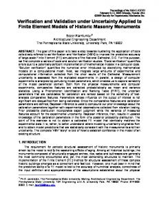
II. Shock Tube Experiment Figure 1 (a) shows the configuration of the shock tube experiment [2]. The shock tube is composed of a 2.1m long driver section, a 5.2m long driven sections and particle curtain test section. The driver section has circular section stainless steel pipe with an inner diameter of 88.9 mm and the driven and test sections have rectangular section aluminum tube having a nominal wall thickness of 12.7mm. The nominal width and height of the driven section are 79.2mm. -4

8

x 10

6

Time (sec)


carried out at Sandia National Laboratories. In particular, it describes the process of UQ and UR that led to exposing model deficiencies followed by model improvement. Compressible Multiphase Turbulence (CMT) has significant importance in many environmental and industrial applications [1]. CMT is common in natural flows such as explosive volcanic eruptions, supernovae, and dust explosions in coal mines and grain silos. In many applications of national defense and security, CMT plays an important role in attempts to predict and control explosive dispersal of particles. To predict CMT dominated behaviors, modeling the physics of shock-particle interaction and particle-particle collision is an important step. Shock tube experiments, where a shock hits a curtain of particles are ideal for testing and validating such models, as the nearly one dimensional nature of flow removes other important effects, such as turbulence. That is, the experimental results are dominated by shock-particle interaction and particle-particle interaction [2,3]. Furthermore, the contributions of the shock-particle and particle-particle interactions can be regulated by changing parameters, which defines initial conditions of the experiment, such as the initial volume fraction of the particles. We can validate the models individually by regulating the experiment initial conditions. The prediction errors of the simulations are composed of the errors in the interaction models and numerical model errors. We identified that the flux calculation model called ASUM+ is the major source of numerical model error and uncertainty using groups of runs. When the physics team replaced AUSM+ by upgrading it to AUSM+up model some surprises were encountered that are described in this paper [7]. This paper is composed of five sections: Section 2 describes the shock tube experiment, the focus of Section 3 is our validation and UQ framework, Section 4 illustrates how the model error can be detected with groups of simulation runs, validation and UQ results before and after the model improvement are presented in Section 5 and Section 6 shows concluding remarks.

2

0 0

(a) Shock tube

Curtain thickness after impact

4

Initial curtain thickness of 2 mm at t=0 0.02

0.04 0.06 Edge location (m)

0.08

0.1

(b) Curves of upstream and downstream particle curtain front positions

(c) Particle curtain before impact (d) Particle curtain after impact Figure 1. Schematic figure of the shock tube



The particle curtain test section has the same sectional dimension with the driven section. The driver and driven sections are separated with a diaphragm with four doors and the pressure difference between two sections generates a shock wave when the diaphragm bursts. The pressure of the driven section was atmosphere pressure and the pressure of driver section is higher than that to generate a shock wave of Mach 1.66. The effect of the different section shape on the shock wave is ignorable. The generated shock wave is stabilized during the travel to the particle test section. Figure 1 (c) and (d) show the side view of the test section, the particle curtain is represented as the black vertical rectangle whose position is defined with left and right front positions. The particle curtain is formed by pouring particles through a slit. The volume fraction of the particle curtain is regulated by pouring speed and the curtain thickness is determined by the slit width. The distance between the two fronts is the particle curtain thickness, which is initially 2 mm before impact of a shock wave. After impact of a shock wave, the particle curtain expands and moves in the direction of the shock wave as shown in Fig. 1 (d). The particle curtain in the test section interacts with the shock and the interaction leads to collisions between particles. 1D simulation is used to predict the behavior of the particle curtain by simulating the experiment with the shockparticle interaction model and particle collision model. The 1D simulation is a simplified version of a CFD code, Rocflu, developed at the Center for Simulation of Advanced Rockets (CSAR) [4,6].

III. Validation and UQ Framework The primary goal of the validation is to discover error in the 1D shock tube simulation by comparing shock tube experiment observations and shock tube simulation predictions. Here we set the modest goal of predicting only the overall behavior of the particle curtain. In terms of finding errors, it is opposite of modest when you look for discrepancies in overall behaviors appeared as prediction metrics (PM). Particle curtain front positions are responses showing the consequence of shock-particle and particle-particle interactions. However, the variability in front positions throughout experiments is uncontrollable. Thus, we set average particle front position curves as PMs. We measured average front positions from 4 repeated experiments. To calculate PMs of the simulation, we identified the sources of uncertainties leading the variation. The variabilities in particle initial position and particle diameter were identified as key uncertainty sources for the experimental variability based on expert opinion. We calculated PMs based on 10 simulations with randomly defined initial particle positions of each simulation. The diameter variation was not considered as inability of the simulation and we are implementing it for future use. That is, discrepancy between PM measured from repeated experiments and PM calculated from repeated simulation is the prediction error due to the inadequacy of the models in the simulation and the current inability of the simulation. The prediction error is a result of superposing all error sources in the simulation and we assume that there are three major error sources: physical model errors, numerical model errors, and discretization error. For example, errors in the particle-shock and particle-particle interaction models are categorized as physical model errors and errors in numerical schemes for calculating flux, density, pressure, etc. are categorized as numerical model errors. Discretization error is error related to grid resolution and the number of particles for the shock-tube simulation. Since the physical model errors are of our primary interest, the effect of other errors should be diagnosed and eliminated from the prediction error. Table 1: Parameters of key uncertainties Parameters Descriptions Bounds Measurement uncertainty in volume Initial condition [18,22] % fraction of a particle curtain uncertainty Diameter of particles Variability [100,130] μm Particle curtain thickness Variability [1.6,2.4] mm Initial particle position Variability The corresponding cell boundary

Nominal values 20% 115μm 2mm -

The measurement uncertainty in volume fraction of a particle curtain is another key uncertainty. Propagating these uncertainties via a process of uncertainty quantification (UQ) is essential for assessing credibility of the validation [8]. We consider measurement uncertainties in measured PM and initial conditions and experimental variability in the shock tube experiment. For example, measured PM varies for different trials due to various uncertainty sources such as variability in initial particle positions, particle diameters, etc. Table 1 lists the key uncertainty sources and their upper and lower bounds. They are assumed to follow uniform distributions with the corresponding bounds. For the 3 American Institute of Aeronautics and Astronautics

initial particle positions, the number of particles are distributed to cells modeling the particle curtain of the simulation. Then the initial particle positions in each cell are randomly distributed within the corresponding cell boundary using a uniform distribution. Experiments

Validation

Numerical Simulation Model Error

Measured Input

Numerical Model Errors

Discretization Error

Measurement Uncertainty

Prediction Error


Physical Model Errors

Measured Position

Uncertainty in Prediction Error

Predicted Position

Sampling Uncertainty

Sampling Uncertainty

Measurement Uncertainty

Propagated Uncertainty

Figure 2: Sources of uncertainties and errors in validation process Figure 2 shows our validation and UQ framework for uncertainty analysis. The measurement uncertainty in inputs denotes uncertainty in initial condition such as the uncertainty in particle curtain volume fraction. The input uncertainty is propagated to quantify the effect of it on the calculated PM. Note that the name, input uncertainty, represents the perspective of simulation such that the simulation inputs should be measured from experiments and their uncertainty can be viewed as output uncertainty in experiment side. Since calculated PM from the simulation was based on 10 simulations and measured PM from experiments was obtained based on 4 repeated experiments, there are sampling uncertainties in the PMs. The sampling uncertainty can be reduced by increasing the number of simulations. The other measurement uncertainty is uncertainty in the measured PM. The front positions were measured from Schlieren images through image processing, so that the uncertainty in the image processing is the measurement uncertainty. But this measurement uncertainty in PM is small [5].

Uncertainty in ypred

Uncertainty in ymeas

ypred

ymeas

Prediction Metric

Uncertainty in prediction error

ymeas-ypred

Prediction error

Figure 3. Calculation process of prediction error and its uncertainty based on measured and calculated PMs and the corresponding uncertainties Because of the uncertainty sources, prediction error is not a deterministic but uncertain. The magnitude of the uncertainty in prediction error defines the confidence of prediction error. Figure 3 shows how to quantify uncertainty in prediction error. The ypred and ymeas are the calculated and measured PMs, respectively. The uncertainties are modeled as random variables. The uncertainty in ypred is the sum of sampling and measurement uncertainties. The uncertainty in ymeas is the sum of sampling and propagated uncertainties. The uncertain prediction error is expressed in terms of the calculated and measured PMs and the corresponding uncertainties as 4 American Institute of Aeronautics and Astronautics

epred   ymeas  esamp ,exp  emeas    ycalc  esamp ,sim  e prop 

(1)

where ymeas is the measurement PM, ycalc is the calculated PM using the simulation, emeas,exp is sampling uncertainty due to 4 experiments, emeas is measurement uncertainty, esamp,sim is sampling uncertainty due to 10 simulations, epred is prediction uncertainty and eprop is propagated uncertainty. Since the uncertainties are independent, the variance of the prediction error is obtained as the sum of the uncertainty variances.

Var  epred   Var  esamp ,exp   Var  emeas   Var  esamp ,sim   Var  eprop 

(2)

The prediction error is decomposed into physical and numerical model errors and discretization error.


epred  ephy ,model  enum,mod el  edisc

(3)

where ephy,model is the physical model error, enum,model is the numerical model error and edisc is the discretization error. Estimating the physical model error is a future goal to with a view to assess the deficiencies of the interaction models. We reduced the large numerical model error hiding the prediction error by canceling other physical errors to focus on the physical model error. The next section will describe how we detected the large numerical model error. Now we working on estimating the discretization error.

IV. Groups of Runs for Detecting Model Error

Figure 4. Sampling points for groups of runs Before applying the validation and UQ framework, we examined the simulation using groups of runs to identify anomalies in simulation consistency such as numerical noise [7]. Since we identified three key parameters, particle diameter, curtain thickness and particle volume fraction, numerical noise in PM for the variation of the parameters will be mixed with other uncertainty sources. We observed the effects of the variations of the parameters on PMs. As noted before, PMs are calculated based on 10 simulations of randomly defined initial particle positions. Figure 4 shows the 20 samples along each of four lines in the three parameter space converging to volume fraction of 23%, diameter of 110μm and curtain thickness of 2.4 mm. The parameters at the converging point were selected because the target point is around the border where the behavior of PM suddenly changes and that is an indicator of simulation inconsistency. Figure 5 shows the average downstream front position at t=50μsec. To present all the groups together, we use the relative distance from the converging point in Fig. 4. At a relative distance of 0 the values are obtained at the converging point so that the values of different groups should have converged to the same value. In contrast, at a relative distance of 1 values are obtained at the other end point of the lines. For example, the value for the diameter line for a relative distance of 1 are at {23%, 100μm, 2.4mm}. 5 American Institute of Aeronautics and Astronautics

55 50 40 35 30 25 20 1

0.8 0.6 0.4 0.2 Relative Distance All parameter Diameter

0

Thickness PVF

55 50 45 40 35

30 25 20 1

0.8 0.6 0.4 0.2 Relative Distance All parameter Diameter

(a) AUSM+

0

Thickness PVF

(b) AUSM+up Figure 5. Groups of simulation runs

It turned out that the numerical model improvement also reduced the noisy model error, which was masquerading as numerical noise. Figure 6 shows zoomed-in behavior of the diameter line for AUSM+ and AUSM+up in the relative distance range of [0.5, 1] corresponding to particle diameter variation within [0.1,0.105] mm. Originally, the random variation in Fig. 6(a) was considered as numerical noise. However, the model improvement also significantly reduced the random variation as Fig. 6(b) shows.

57.6

28.2

Average Downstream Front Position (mm)



45

60


60


Figure 5(a) shows that the behavior along the line of diameter variation is significantly different from the behavior along the other lines and the discontinuity in its trend did not have a physical explanation. The physics team identified the most likely cause of the behavior in the use of AUSM+ scheme, a numerical flux calculation scheme [9]. In the simulation, Lagrangian particles travel in the grids and flux calculation has to consider the effect of particles in gas. AUSM+ assumes particles in one cell are evenly distributed but the assumption provokes numerical instability with unknown reason when particles in one cell are extremely concentrated. Consequently the flux calculation model that AUSM+ scheme was upgraded to AUSM+up scheme to take into account of particle concentration in a cell [10]. Figure 5(b) shows that the upgrade led to significant model error reduction and the behaviors of different groups becasme consistent. The numerica model improvement reduced the numerical model error.

57.3 57.0 56.7 56.4 0.0995 0.1015 0.1035 0.1055 Particle Diameter (mm)

27.9 27.6 27.3 27.0 0.0995 0.1015 0.1035 0.1055 Particle Diameter (mm)

(a) AUSM+ (b) AUSM+up Figure 6. Behavior of the diameter line for relative distance range of [0.5, 1] 6 American Institute of Aeronautics and Astronautics

V. Validation and UQ Results Figure 7(a) and (b) show 1) calculated PM, average downstream and upstream particle curtain front positions based on 10 simulations, using the 1D simulation and the corresponding propagated uncertainty (red and blue error bands) and 2) measured PM based on 4 experiments and the corresponding sampling uncertainty for 1D AUSM+ and 1D AUSM+up. The bandwidth, which is the 95% confidence interval of the uncertainty, is expressed as a function of time. -4

-4

8

x 10

8

6 Time (sec)

Time (sec)

6

4

4

2

2

0 0 0.02 0.04 0.06 0.02 0.04 0.06 0.08 Front Position (m) Front Position (m) (a) 1D AUSM+ (b) 1D AUSM+up Figure 7. Quantified uncertainties

0 0

0.08

An interesting observation from Fig. 7 is that the model improvement and reducing the model error increased the discrepancy between simulations and experiments. The reduction in model uncertainty was reflected in the bandwidth reduction of the downstream front location. This tells that the error in AUSM+ and the other errors in the particle force and collision models were compensating for one another and it gave the wrong impression that the disagreement between simulation and experiment (prediction error) was small. This observation indicates that good agreement between simulations and experiments is not always a good measure of the prediction capability because errors compensating for one another lead to good agreement. -4

8

-4

x 10

8

4

2

0 0

x 10

6 Time (sec)

6 Time (sec)


x 10

4

2

0 0.02 0.04 0.06 0.08 0 0.02 0.04 0.06 Front Position (m) Front Position (m) (a) 1D AUSM+up (b) 2D AUSM+ Figure 8. Quantified uncertainties


0.08

-4

8

-4

x 10

8

time (sec)

4

4

2

2 95% CI of DFP 95% CI of UFP 0

x 10

6

6

Time (sec)


Since the experiment is not truly one-dimensional, we are now moving to examine 2D and 3D simulations. Figure 8(a) and (b) show calculated and measured PMs of 1D AUSM+up and 2D AUSM+. Note that 2D simulation showed uses AUSM+ and it will be upgraded to AUSM+up. From the experience with the 1D simulation, the small disagreement of 2D simulation is not may also be caused by the compensating errors and the magnitude will possibly be significantly larger as AUSM+ will be upgraded. This suggested a need to accelerate the implementation schedule of 2D AUSM+up. The prediction errors of 1D AUSM+ and 1D AUSM+up simulations were obtained using Eq. (1) as a function of time. The corresponding prediction errors and its uncertainties are presented in Fig. 9. The uncertainty in prediction error is plotted in a format of 95% confidence interval. Figure 10 shows the contributions of uncertainty sources on the uncertainty in prediction errors: sampling uncertainty, experimental sampling uncertainty and propagated uncertainty, to the model uncertainty. Since, in the validation and UQ framework, the uncertainties are independent, we decompose the contributions using their variances. The total variance of the uncertainty in the prediction error is calculated using Eq. (2). Since the bandwidth represents the total variance, the band can be decomposed using the individual variances and the total variance. The contributions of individual uncertainties are presented in different colors and the bands of the plots in Fig. 9 are decomposed into different colors as Fig. 10. Figure 10(a) and (b) show uncertainty contributions of the uncertainty in prediction errors of the 1D AUSM+. Note that we do not show the measurement uncertainty of the experiment data in the plots since it is very small [5]. The contribution of using 10 simulations to obtain PM, which is the average front positions, is the simulation sampling uncertainty.. The uncertainty in the prediction error mostly comes from the sampling uncertainty for the downstream curtain front position. This result indicates that variability due to initial particle position variation is much larger than that of AUSM+up. If we consider that the same experiment data is used for validation and UQ of both simulations, the 1D AUSM+up scheme is less sensitive to the initial particle position variation than the 1D AUSM+. Figure 10(c) and (d) show contributions of uncertainty sources to the uncertainty in prediction errors of 1D AUSM+up. In contrast to the 1D AUSM+ results, the uncertainty in the downstream curtain front position mostly comes from the propagated uncertainty, which is a resultant uncertainty of initial condition uncertainty. Also the simulation sampling uncertainty is little, decreasing the number of random simulation runs can save computation resources while the uncertainty increment is small compared to the effects of other uncertainty sources. The uncertainty of the upstream curtain front position prediction comes from the experimental sampling uncertainty and propagated uncertainty equally. In other words, to reduce the uncertainty in the downstream curtain front location, we need to reduce the uncertainty in initial conditions. To reduce the uncertainty in upstream curtain front location, both uncertainties should be reduced.

0

5 10 15 Prediction error in edge location (mm)

0

20

95% CI of DFP 95% CI of UFP 0

5 10 15 20 Prediction error in edge location (mm)

(a) 1D AUSM+ (b) 1D AUSM+up Figure 9. Prediction errors of 1D AUSM+ and AUSM+up Since reducing the various uncertainties requires expenditure of time and money, one important future goal is to quantify the uncertainty reduction budgets of the uncertainty sources. For example, measurement uncertainty in volume fraction is uncertainty in initial conditions and reducing the uncertainty requires cost for better equipment. If we have set a target of reducing our total uncertainty by 25%, UR budget for achieving this target is referred as 8 American Institute of Aeronautics and Astronautics

uncertainty budget (UB). Thus we can plan to efficiently reduce uncertainty based on estimated cost and time of the various measure of reducing uncertainties. Also a 3D simulation is being prepared to consider the 3D effects in the shock-tube experiment, which are ignored in 1D simulation. UQ of the 3D simulation will be carried out in the future. Since UQ requires computational resource more than one order of simulation, UQ of the 3D simulation is computationally very expensive. To tackle this problem, a multi-fidelity surrogate model will be applied for 3D validation to compensate small amount of expensive 3D simulation data with large amount of cheap 1D and 2D simulation data. -4

8

-4

x 10

8

Time (sec)

Time (sec)

6

4

Sampling uncertainty (Sim) Sampling uncertainty (Exp) Prop. Uncertainty

2

0

0

5 10 Error in edge location (mm)

4

0


15

-4

x 10

8

x 10

6

Time (sec)

6

4

2

0

0

(b) Prediction error for downstream position (1D AUSM+)

-4

8


2

15

(a) Prediction error for upstream position (1D AUSM+)

Time (sec)


6

x 10

Sampling uncertainty (Sim) Sampling uncertainty (Exp) Prop. Uncertainty 0


15

4


2

0

0


15

(c) Prediction error for upstream position (d) Prediction error for downstream position (1D AUSM+up) (1D AUSM+up) Figure 10. Model uncertainty and the sources of the uncertainty

VI. Concluding Remarks The paper described the process of uncertainty quantification and reduction for the purpose of validation of a simulation code for compressible multiphase flow. In particular, we focused on simulation and experiments for a shock hitting a curtain of particles in a shock tube. We described the process of identifying the major uncertainties in input and output and propagating their effects by multiple simulations in the uncertain parameter space. Different arrangements of the parameters space points allowed us to uncover anomalies and noise in the simulations. Prior papers about simulation validation have focused on prediction capability assessment in terms of the agreement between a simulation and experimental data and quantifying its credibility through UQ. However, this paper found that good agreement may be due to errors compensating for one another. In particular results indicated that a numerical model error may have compensated for physical model error for 1D shock tube simulation validation. Gas flux numerical model improvement exposed model deficiency possibly due to errors in two important physics models, 9 American Institute of Aeronautics and Astronautics

particle collision and force models. A second surprising result found was that the apparent numerical noise in the 1D simulation turned out to be due to the same flux model error, as the noise was significantly reduced by the model improvement.

Acknowledgements This work is supported by the U.S. Department of Energy, National Nuclear Security Administration, Advanced Simulation and Computing Program, as a Cooperative Agreement under the Predictive Science Academic Alliance Program, under Contract No. DE-NA0002378.

References 1

Zhang, F., et al. "Explosive dispersal of solid particles." Shock Waves 10.6 (2001): 431-443.


2 Wagner, J. L., Beresh, S. J., Kearney, S. P., Trott, W. M., Castaneda, J. N., Pruett, B. O., & Baer, M. R. (2012). A multiphase shock tube for shock wave interactions with dense particle fields. Experiments in fluids, 52(6), 15071517. 3

Wagner, J. L., Beresh, S. J., Kearney, S. P., Pruett, B. O., & Wright, E. K. (2012). Shock tube investigation of quasi-steady drag in shock-particle interactions. Physics of Fluids (1994-present), 24(12), 123301. 4

Rocstar Softwar Suite. (n.d.). Retrieved from http://www.csar.illinois.edu/rocstar/index.html

5

Justin Wagner, personal communication, March 26, 2014.

6 Ling, Y., Wagner, J. L., Beresh, S. J., Kearney, S. P., & Balachandar, S. (2012). Interaction of a planar shock wave with a dense particle curtain: Modeling and experiments. Physics of Fluids (1994-present), 24(11), 113301. 7 Fernandez-Godino, M. G., Diggs, A., Park, C., Kim, N. H., Haftka, T. R. (2016) Anomaly Detection via Groups of Simulations, 18th AIAA Non-Deterministic Approaches Conference, San Diego, CA, USA, 4-8 January 2016. 8 Oberkampf, W. L., & Roy, C. J. (2010). Verification and validation in scientific computing. Cambridge University Press.

Liou, M.-S., “A sequel to ausm: Ausm+,” Journal of computational Physics, Vol. 129, No. 2, 1996, pp. 364–382.

9

10

Liou, M. S., Chang, C. H., Nguyen, L., & Theofanous, T. G. (2008). How to solve compressible multifluid equations: a simple, robust, and accurate method. AIAA journal, 46(9), 2345-2356.
