Value Ordering for Offline and Realtime-Online

Value Ordering for Offline and Realtime-Online Solving of Quantified Constraint Satisfaction Problems DAVID S TYNES

A Thesis Submitted to the National University of Ireland in Fulfillment of the Requirements for the Degree of Doctor of Philosophy in Computer Science.

November, 2009

Research Supervisor: Dr. Kenneth N. Brown. Head of Department: Prof. James Bowen

Department of Computer Science, National University of Ireland, Cork.

Contents Abstract

viii

1 Introduction

1

1.1

The Constraint Satisfaction Problem . . . . . . . . . . . . . . . .

1

1.2

The Quantified Constraint Satisfaction Problem . . . . . . . . . .

3

1.3

Contributions of this Thesis . . . . . . . . . . . . . . . . . . . . .

4

1.4

Thesis Outline . . . . . . . . . . . . . . . . . . . . . . . . . . . .

5

2 Literature Review

7

2.1

Introduction . . . . . . . . . . . . . . . . . . . . . . . . . . . . .

7

2.2

Constraint Satisfaction Problems . . . . . . . . . . . . . . . . . .

7

2.2.1

Constraint Propagation . . . . . . . . . . . . . . . . . . .

9

2.2.2

Backtracking Search . . . . . . . . . . . . . . . . . . . . 11

2.2.3

Variable and Value Ordering Heuristics . . . . . . . . . . 15

2.3

2.4

Quantified Constraint Satisfaction Problems . . . . . . . . . . . . 19 2.3.1

Fundamental Notions and Properties of QCSP . . . . . . . 21

2.3.2

Propagation in QCSPs . . . . . . . . . . . . . . . . . . . 26

2.3.3

Search in QCSPs . . . . . . . . . . . . . . . . . . . . . . 34

2.3.4

QCSP-Solve . . . . . . . . . . . . . . . . . . . . . . . . 38

2.3.5

Modeling Difficulties in QCSP . . . . . . . . . . . . . . . 42

2.3.6

Relaxations and Explanations for QCSP . . . . . . . . . . 45

2.3.7

Variable and Value Ordering Heuristics in QCSPs . . . . . 46

Online CSP . . . . . . . . . . . . . . . . . . . . . . . . . . . . . 47 2.4.1

Dynamic CSP . . . . . . . . . . . . . . . . . . . . . . . . 51

2.4.2

Mixed CSP . . . . . . . . . . . . . . . . . . . . . . . . . 52 i

2.4.3

Branching CSP . . . . . . . . . . . . . . . . . . . . . . . 52

2.4.4

Probabilistic and Stochastic CSP . . . . . . . . . . . . . . 53

2.4.5

AI Game Playing . . . . . . . . . . . . . . . . . . . . . . 54

2.5

Online Bin Packing . . . . . . . . . . . . . . . . . . . . . . . . . 60

2.6

Summary . . . . . . . . . . . . . . . . . . . . . . . . . . . . . . 62

3 Value Ordering Heuristics for QCSP

63

3.1

Introduction . . . . . . . . . . . . . . . . . . . . . . . . . . . . . 63

3.2

Solution-focused Adversarial Heuristics . . . . . . . . . . . . . . 64 3.2.1

Experiments: Adversarial Heuristics . . . . . . . . . . . . 67

3.3

Verification-focused Pure Value Heuristics . . . . . . . . . . . . . 78

3.4

Higher Density Problems . . . . . . . . . . . . . . . . . . . . . . 85

3.5

Conclusions . . . . . . . . . . . . . . . . . . . . . . . . . . . . . 87

4 Realtime Online Solving of Quantified CSPs

90

4.1

Introduction . . . . . . . . . . . . . . . . . . . . . . . . . . . . . 90

4.2

Realtime Online Solving of QCSP . . . . . . . . . . . . . . . . . 92

4.3

Realtime Online solving of QCSP Through Game-Tree Search . . 94 4.3.1

4.4

Overall Approach . . . . . . . . . . . . . . . . . . . . . . 95

Experiments . . . . . . . . . . . . . . . . . . . . . . . . . . . . . 119 4.4.1

Empirical Evaluation when the Universal Actor is Adversarial . . . . . . . . . . . . . . . . . . . . . . . . . . . . 122

4.5

4.4.2

Empirical Evaluation when the Universal Actor is Random 125

4.4.3

Empirical Evaluation when the Universal Actor is Benevolent . . . . . . . . . . . . . . . . . . . . . . . . . . . . 127

4.4.4

Experimental Summary . . . . . . . . . . . . . . . . . . 128

Conclusions . . . . . . . . . . . . . . . . . . . . . . . . . . . . . 130

5 Realtime Online Solving of QCSPs applied to Online Bin Packing

132

5.1

Introduction . . . . . . . . . . . . . . . . . . . . . . . . . . . . . 132

5.2

Modeling with Shadow Variables . . . . . . . . . . . . . . . . . . 133 5.2.1

5.3

Introducing Shadow Variables to a Model . . . . . . . . . 134

Modeling Online Bin Packing . . . . . . . . . . . . . . . . . . . 142 5.3.1

Type-1 problems . . . . . . . . . . . . . . . . . . . . . . 144 ii

5.4

5.3.2 Type-2 problems . . . . . . . . . . . . . . . . . . . . . . 147 Realtime Online Solving of Online Bin Packing QCSPs . . . . . . 149

5.5

5.4.1 Heuristics for Online Bin Packing . . . . . . . . . . . . . 149 5.4.2 Constraint Propagation for Non-Binary QCSPs . . . . . . 153 Experimental Evaluation on Online Bin Packing Problems . . . . 158 5.5.1 5.5.2

5.6

Type-1 Problems - Experimental Results . . . . . . . . . 161 Type-2 Problems - Experimental Results . . . . . . . . . 167

5.5.3 Improving the Universal Actor . . . . . . . . . . . . . . . 172 5.5.4 Testing Against a MinSpace Universal . . . . . . . . . . . 174 Conclusions . . . . . . . . . . . . . . . . . . . . . . . . . . . . . 176

6 Conclusions and Future Work 6.1 6.2

178

Conclusions . . . . . . . . . . . . . . . . . . . . . . . . . . . . . 178 Future Work . . . . . . . . . . . . . . . . . . . . . . . . . . . . . 181

Bibliography

184

iii

List of Figures 2.1

Illustration of the notions of Solution,Scenario,Winning Strategy and Outcome on the QCSP ∃x1 ∀x2 ∃x3 , D1 = {2, 3}, D2 = {3, 4}, D3 = {3, 4, 5, 6}, C = {(x1 + x2 ≤ x3)} . . . . . . . . . . . . . . . . . 24

3.1 3.2

n = 21, n∀ = 7, d = 8, p = 0.20, q∀∃ = 1/2 . . . . . . . . . . . . 70 n = 21, n∀ = 7, d = 8, p = 0.20, q∀∃ = 1/2 . . . . . . . . . . . . 70

3.3

n = 24, b = 1, d = 8, p = 0.20, q∀∃ = 1/2 . . . . . . . . . . . . . 74

3.4

n = 24, b = 1, d = 8, p = 0.20, q∀∃ = 1/2 . . . . . . . . . . . . . 75

3.5 3.6

n = 21, n∀ = 7, d = 8, p = 0.20, q∀∃ = 1/2 . . . . . . . . . . . . 75 n = 24, b = 1, d = 8, p = 0.20, q∀∃ = 1/2 . . . . . . . . . . . . . 76

3.7

n = 24, n∀ = 8, d = 8, p = 0.14, q∀∃ = 1/2 . . . . . . . . . . . . 77

3.8 3.9

n = 21, n∀ = 7, d = 8, p = 0.20, q∀∃ = 1/2 . . . . . . . . . . . . 82 n = 21, n∀ = 7, d = 8, p = 0.20, q∀∃ = 1/2 . . . . . . . . . . . . 82

3.10 n = 24, b = 1, d = 8, p = 0.20, q∀∃ = 1/2 . . . . . . . . . . . . . 83 3.11 n = 24, b = 1, d = 8, p = 0.20, q∀∃ = 1/2 . . . . . . . . . . . . . 84 3.12 n = 21, n∀ = 7, d = 8, p = 0.40, q∀∃ = 1/2 . . . . . . . . . . . . 86 3.13 n = 21, n∀ = 7, d = 8, p = 0.40, q∀∃ = 1/2 . . . . . . . . . . . . 86 3.14 n = 22, b = 1, d = 8, p = 0.70, q∀∃ = 1/2 . . . . . . . . . . . . . 87 3.15 n = 22, b = 1, d = 8, p = 0.70, q∀∃ = 1/2 . . . . . . . . . . . . . 88 4.1 4.2

∀x∃y∀z∃w, Dx = Dy = Dz = Dw = {1, 2, 3, 4, 5, 6} . . . . . . . 98 Depth-First Tree Traversal . . . . . . . . . . . . . . . . . . . . . 106

4.3

Breadth-First Tree Traversal . . . . . . . . . . . . . . . . . . . . 107

4.4 4.5

Best-First Tree Traversal . . . . . . . . . . . . . . . . . . . . . . 108 Partial Best-First Tree Traversal . . . . . . . . . . . . . . . . . . 109

4.6

Alpha Beta Pruning Tree Traversal . . . . . . . . . . . . . . . . . 110 iv

4.7

Intelligent Depth-First Tree Traversal . . . . . . . . . . . . . . . 111

4.8

n = 20, b = 1, d = 8, p = 0.20, q∀∃ = 1/2, T imeLimit = 1000ms . . . . . . . . . . . . . . . . . . . . . . . . . . . . . . . 122

4.9

n = 20, b = 1, d = 8, p = 0.20, q∀∃ = 1/2, T imeLimit = 1000ms . . . . . . . . . . . . . . . . . . . . . . . . . . . . . . . 123

4.10 n = 20, b = 1, d = 8, p = 0.20, q∀∃ = 1/2, T imeLimit = 1000ms . . . . . . . . . . . . . . . . . . . . . . . . . . . . . . . 124 4.11 n = 51, b = 1, d = 8, p = 0.20, q∀∃ = 1/2, T imeLimit = 1000ms . . . . . . . . . . . . . . . . . . . . . . . . . . . . . . . 125 4.12 n = 51, b = 1, d = 8, p = 0.20, q∀∃ = 1/2, T imeLimit = 1000ms . . . . . . . . . . . . . . . . . . . . . . . . . . . . . . . 126 4.13 n = 20, b = 1, d = 8, p = 0.20, q∀∃ = 1/2, T imeLimit = 500ms . . . . . . . . . . . . . . . . . . . . . . . . . . . . . . . 127 4.14 n = 20, b = 1, d = 8, p = 0.20, q∀∃ = 1/2, T imeLimit = 500ms

. . . . . . . . . . . . . . . . . . . . . . . . . . . . . . . 128

4.15 n = 20, b = 1, d = 8, p = 0.20, q∀∃ = 1/2, T imeLimit = 500ms . . . . . . . . . . . . . . . . . . . . . . . . . . . . . . . 129 4.16 n = 20, b = 1, d = 8, p = 0.20, q∀∃ = 1/2, T imeLimit = 500ms . . . . . . . . . . . . . . . . . . . . . . . . . . . . . . . 129 5.1

Behaviour of Ordered Fitting (OF) . . . . . . . . . . . . . . . . . 150

5.2

Behaviour of Heavily Filled (HF) . . . . . . . . . . . . . . . . . . 151

5.3

Behaviour of Best Fit (BF) on the packet ordering 2, 1, 8 . . . . . 152

5.4

Type-2 problems: m = 4, k = 2, c = 10, tl∃ = 1000ms . . . . . . 160

5.5

Type-1 problems: m = 4, k = 2, c = 10, tl∃ = 1000ms . . . . . . 161

5.6

Type-1 problems: m = 5, k = 3, c = 8, tl∃ = 1000ms

5.7

Type-1 problems: m = 10, k = 6, c = 10, tl∃ = 1000ms . . . . . 163

5.8

Type-1 problems: m = 10, k = 6, c = 10, tl∃ = 5000ms . . . . . 164

5.9

Type-1 problems: m = 4, k = 2, c = 10, tl∃ = 1000ms . . . . . . 164

5.10 Type-1 problems: m = 5, k = 3, c = 8, tl∃ = 1000ms

. . . . . . 162

. . . . . . 165

5.11 Type-1 problems: m = 10, k = 6, c = 10, tl∃ = 1000ms . . . . . 166 5.12 Type-2 problems: m = 4, k = 2, c = 10, tl∃ = 1000ms . . . . . . 167 5.13 Type-2 problems: m = 5, k = 3, c = 8, tl∃ = 1000ms v

. . . . . . 168

5.14 Type-2 problems: m = 4, k = 2, c = 10, tl∃ = 1000ms . . . . . . 169 5.15 Type-2 problems: m = 5, k = 3, c = 8, tl∃ = 1000ms . . . . . . 170 5.16 Type-2 problems: m = 10, k = 6, c = 10, tl∃ = 1000ms . . . . . 170 5.17 Type-2 problems: m = 10, k = 6, c = 10, tl∃ = 1000ms . . . . . 171 5.18 Type-1 problems: m = 10, k = 6, c = 10, tl∃ = 1000ms . . . . . 173 5.19 Type-2 problems: m = 10, k = 6, c = 10, tl∃ = 1000ms . . . . . 174 5.20 Type-1 problems: m = 10, k = 6, c = 10, tl∃ = 1000ms . . . . . 175 5.21 Type-1 problems: m = 10, k = 6, c = 10, tl∃ = 5000ms . . . . . 176

vi

List of Tables 5.1 5.2 5.3

Constraint R . . . . . . . . . . . . . . . . . . . . . . . . . . . . . 136 Tuple (a) added to constraint sR . . . . . . . . . . . . . . . . . . 137 Tuple (b) added to constraint sR . . . . . . . . . . . . . . . . . . 137

5.4 5.5

Constraints R1 and R2 . . . . . . . . . . . . . . . . . . . . . . . 140 Constraint sR1+2 . . . . . . . . . . . . . . . . . . . . . . . . . . 140

vii

Abstract

Standard Constraint Satisfaction Problems (CSPs) are not suited to reasoning on problems containing uncertainty or adversarial situations (e.g. games), in which the decisions are not all under the control of a single decision maker. We can describe these types of problems as online CSPs, where the problem variables must be instantiated in a fixed sequence, but where some of those variables are set externally. There exists an extension of CSP, the Quantified Constraint Satisfaction Problem (QCSP), which can be regarded as a model for these types of online CSP. A QCSP allows the variables to be universally or existentially quantified, and to solve a QCSP we must find a strategy that allows a solution to be reached no matter what combination of values the universally quantified variables may take. Finding a winning strategy to the QCSP guarantees being able to reach a solution in the online CSP. Unfortunately, solving the QCSP is, in general, PSPACE-complete. As such when the problem size is increased, even the most efficient QCSP solvers quickly become unable to solve the problem. In this dissertation, we investigate the use of Value Ordering Heuristics to help address this issue. We show that value ordering can be used to improve the efficiency of search when solving QCSPs. For cases where the online CSP is also real time, i.e. the decisions must be made within strict time limits and we do not have enough time to fully solve the QCSP, we investigate an approach in which we use value ordering to help us reason about what value to pick for the current decision. We perform game-tree search augmented with constraint propagation during our limited time per decision, and use the value ordering heuristics to evaluate the states explored during the search to help choose what value to assign the current variable. We show that both on randomly generated binary QCSPs and on Online Bin Packing problems we can achieve good performance with this approach, and can also handle QCSP problem instances which are too large to solve fully.

viii

Declaration This dissertation is submitted to University College Cork, in accordance with the requirements for the degree of Doctor of Philosophy in Computer Sciencein the Faculty of Science. The research and thesis presented in this dissertation are entirely my own work and have not been submitted to any other university or higher education institution, or for any other academic award in this university. Where use has been made of other people’s work, it has been fully acknowledged and referenced. Parts of this work have appeared in the following publications which have been subject to peer review: David Stynes and Kenneth N. Brown. Value Ordering for Quantified CSPs. In Proceedings of CP2007 Doctoral Programme, pages 157-162, 2007. David Stynes and Kenneth N. Brown. Realtime Online Solving of Quantified CSPs. In Proceedings of Workshop on Quantification in Constraint Programming,QiCP, 2008. David Stynes and Kenneth N. Brown. Value Ordering for Quantified CSPs. Constraints, 14(1):16-37,2009. David Stynes and Kenneth N. Brown. Realtime Online Solving of Quantified CSPs. In Proceedings of CP, pages 771-786, 2009.

The contents of this dissertation extensively elaborate upon previously published work and mistakes (if any) are corrected. Large sections of this work are previously unpublished, although they may appear in some journals in the future.

David Stynes September 2009.

ix

Dedication This dissertation is unimaginatively dedicated to my family and close friends.

x

Acknowledgements I would first like to thank my supervisor, Ken Brown, for his invaluable support, guidance and insight in helping me to complete the work compiled within this dissertation. I would also like to thank the many members of the Cork Constraint Computation Centre (4C), who have helped shape my understanding of the many facets of constraint programming. And also to thank the members of Microsoft Research Cambridge, in particular my research mentors, Youssef Hamadi and Lucas Bordeaux, for their suggestions. This work was supported in part by Microsoft Research through the European PhD Scholarship Programme, and by the Embark Initiative of the Irish Research Council for Science, Engineering and Technology (IRCSET).

xi

Chapter 1 Introduction The thesis defended in this dissertation is that: Value Ordering can enhance Quantified Constraint Satisfaction Problem solving. In particular: 1. when solving an entire QCSP, effective value ordering improves the efficiency of the search. 2. when reasoning on QCSPs interactively under time constraints, value ordering in combination with AI Game Playing adversarial reasoning allows the participants to achieve their objectives more frequently.

1.1 The Constraint Satisfaction Problem Quantified Constraint Satisfaction Problems are an extension of Constraint Satisfaction Problems(CSP). We will start by first introducing CSPs. An instance of a CSP consists of a finite set of variables, domains for those variables and a set of constraints, restricting which values the variables may take. A solution to the CSP is a function, mapping values from their domains to all of the variables, such that all of the constraints are satisfied. Each Constraint is a relation over a subset of the variables. As an example of a CSP, we give a simple problem. We seek to find the sum (MONEY) of two numbers (SEND and MORE). Each of the letters M, O, N, E, Y, S, D and R is a distinct digit 0...9. 1

SEND +MORE MONEY

A typical representation of this problem as a CSP is as follows. Each of the letters is represented as a variable. Variables S and M are both the first digits of numbers, so their domains are {1..9}, while the remaining variables have domains {0..9}. Since the letters must be distinct, an all-different constraint is applied to

all the variables, forcing them to all take a distinct value. Then the constraint to find the sum can be expressed as:

1000 × S + 100 × E + 10 × N + 1 × D +1000 × M + 100 × O + 10 × R + 1 × E = 10000 × M + 1000 × O + 100 × N + 10 × E + 1 × Y A solution satisfying these constraints would be: S = 9, E = 5, N = 6, D = 7, M = 1, O = 0, R = 8, Y = 2. CSPs are in general intractable, they are NP-Complete[1]. Finding a solution is performed via backtracking search, which exhaustively explores all combinations of value assignments to the variables until a solution is found. Constraint propagation is used throughout search to prune parts of the search space which are proven to not contain solutions. CSPs have been successfully applied to solve problems in a wide variety of fields including: Scheduling[45], Graph Coloring[69], Boolean Satisfiability[102], Temporal Reasoning[104], Bin Packing and Partitioning[53] and Frequency Allocation[72]. 2

1.2 The Quantified Constraint Satisfaction Problem CSPs assume we have complete control over the problem and can assign the variables any value we choose. In many problems this may not be the case, other actors or the environment itself may take actions which affect our decisions, but we do not know in advance what action they will take. Quantified Constraint Satisfaction Problems(QCSP) are an extension of CSP which allows problems with such uncertainty to be modeled compactly. In a CSP, all of the variables are implicitly existentially quantified. In a QCSP, variables are explicitly either existentially (∃) or universally (∀) quantified. The existentially quantified variables are those for which we can decide their assignment, while the universally quantified variables are those for which we are required to support every value in their domains. Solving a QCSP requires finding a strategy of assignments to each of the existential variables, based upon on the values of the universal variables before it in the variable sequence, that guarantees reaching a solution regardless of what possible combination of values may have been assigned to the universally quantified variables. A solution to a QCSP is the same as that of a CSP: a mapping of values to the variables such that all the constraints are satisfied. An instance of a QCSP consists of a finite set of variables, domains for those variables, a set of constraints and a sequence of quantifiers, one for each variable, which defines an ordering on the variables. Below we provide a sample QCSP:

∃x1 ∀y1 ∃x2 , Dx1 = Dy1 = Dx2 = {1, 2, 3}, all-different(x1 , y1, x2 ) We have 3 variables, x1 , y1 , x2 in which x1 and x2 are existentially quantified, and y1 is universally quantified. All three share the domain {1, 2, 3} and there is a

constraint stating that the 3 variables must take distinct values. The quantifiers can be read as meaning, ”there exists a value for x1 such that for any value of y1 we can find a value for x2 which satisfies the constraints”. If this were a CSP (i.e. all

variables existentially quantified) then a solution would be x1 = 1, y1 = 2, x2 = 3. But as a QCSP, this problem is unsatisfiable: there is no strategy to assign a value 3

to x1 which supports every value in the domain of y1 , since y1 can always take the same value x1 took, violating the all-different constraint. Due to the need to find a strategy for all combinations of values that the universally quantified variables may take, the complexity of QCSPs in general is PSPACE-Complete[22], though many polynomial-time tractable cases have also been identified[35]. As a result of this complexity, solving QCSPs in reasonable time quickly becomes infeasible as the size of problems increases. Techniques from various fields have been employed to improve the efficiency of QCSP Solvers, such as: the Pure Value Rule and Solution Directed Pruning originating from Quantified Boolean Formulae, Constraint Propagation, Backjumping and Neighborhood Interchangeability originating from CSP. Ordering Heuristics, for selecting which variable to assign next or which value to assign to the current variable, have been one of the most useful techniques for improving the efficiency of CSPs. However no study on what is required for the extension of value ordering heuristics to QCSP from CSP had been presented prior to the work which is presented as part of this dissertation[108, 111].

1.3 Contributions of this Thesis The goal of this thesis is to enhance the current state of Quantified Constraint Satisfaction Problem solving through the use of Value Ordering Heuristics. This is the primary contribution of this thesis and it is split into two parts: 1. when solving an entire QCSP, we show that effective value ordering improves the efficiency of the search reducing the number of search nodes explored, and the time taken to solve the QCSP. We identify two non-distinct families of value ordering heuristics for solving QCSPs: Solution-focused, in which we pick values based on whether or not they lead to a solution, and Verification-focused, in which we pick values which can be most quickly confirmed as being part of a winning strategy or not. 2. It is possible to be faced with a QCSP which is impossible to fully solve, as we are provided limited time which is insufficient for the search to be completed. In this circumstance we show if we reason interactively on the 4

QCSP under time constraints in response to the decisions made by the other actors, we can use value ordering in combination with AI Game Playing adversarial reasoning to allow the participants of the problem to achieve their objectives more frequently. Secondary contributions of this thesis are: • A problem generator for random binary QCSPs which does not generate any of the flaws described in[62]. • A new lookahead strategy, Partial Best First, for reasoning when performing realtime online solving of QCSPs under time constraints. • Three new notions of consistency: Existential Quantified Arc Consistency (EQAC) for binary QCSPs and two for non-binary constraints, Quantified Non-binary Forward Checking (QnFC0) and Existential Quantified Generalised Arc Consistency (EQGAC) • An automated system for generating Shadow Variable models from standard models, to allow for illegal values to be pruned from universally quantified domains. • Two models for variants of Online Bin Packing Problems as QCSPs. • Three value ordering heuristics: Ordered Fitting, Heavily Fitted and MinSpace, for use on online bin packing QCSPs.

1.4 Thesis Outline The remainder of this thesis is laid out as follows: Chapter 2 We present a review of the relevant literature. Chapter 3 We develop the use of Value Ordering Heuristics for solving QCSPs. We identify two families of value ordering heuristics and identify classes of QCSP for which each is suitable. 5

Chapter 4 We develop a game-tree search based approach for performing Realtime Online Solving of QCSPs, where decisions must be made under timelimited circumstances and there is not time for solving the entire QCSP. We test this approach on randomly generated binary QCSPs. Chapter 5 We apply our game-tree search approach for realtime online solving of QCSPs to a practical application, Online Bin Packing problems. We show that the approach shows promise on these problems and not just on randomly generated binary QCSPs. Chapter 6 We present our conclusions and describe our future work.

6

Chapter 2 Literature Review 2.1 Introduction In this chapter we review work related to this thesis. It is divided into 3 sections. Firstly we review the relevant literature on Constraint Satisfaction Problems. Then we describe in detail the current state of Quantified CSP. We then briefly look at related extensions of CSP which handle reasoning under uncertainty, dynamic problems where the problem changes over time, and realtime online situations, where we must respond rapidly to received information.

2.2 Constraint Satisfaction Problems As already stated, QCSP is an extension of CSP. As such, many of the methods used in solving QCSPs are extensions from those of CSPs. In this section we review the relevant core practices of CSP solving, starting by defining a CSP. Definition 2.2.1 (Constraint Satisfaction Problem (CSP)). A CSP is a triple P =

(X ,D,C). It consists of a finite set of n variables X = {x1 , .., xn }, a finite set of n domains for those variables D = {D1 , .., Dn } where Di is the domain of xi and a finite set of constraints C = {C1 , .., Ce }. To understand the semantics of Definition 2.2.1 some additional definitions are also needed. 7

Definition 2.2.2 (Variable). Each variable xi represents a decision in the problem and must be assigned a value which does not conflict with the values assigned to other variables. Definition 2.2.3 (Domain of a Variable). Each domain Di is the domain of variable xi and is the set of possible values that xi may be assigned. Values in a domain do not necessarily satisfy all constraints, and may not be a part of any solution. Definition 2.2.4 (CSP Constraint). In a CSP P = (X ,D,C), a constraint Ck ∈ C is defined over a subset, Xk , of the variables in X , where Xk = {xk1 , .., xkl }. Ck

has an associated set CkS ⊆ Dk1 × .. × Dkl of tuples which specifies the allowed combinations of values for the variables in Xk . The arity of a constraint is |Xk |, the number of variables it is defined over. A k-ary constraint is a constraint over k variables, and a binary constraint is a constraint over 2 variables. When discussing a single constraint, the subscript will often be used to indicate which variables it restricts, i.e. Cij is a binary constraint over the variables xi and xj . Definition 2.2.5 (Variable Assignment). A variable assignment (also called an instantiation) (x, a) is a variable-value pair which represents the assignment of value a to variable x. An instantiation of a set of variables is a tuple of ordered pairs, where each ordered pair (xi , ai ) represents the assignment of value ai to variable xi . In a CSP P = (X ,D,C), such a tuple t = ((x1 , a1 ),..,(xj , aj )) is said to satisfy a constraint Ck if all the variables of Xk are in the tuple, and their combined assigned values for the variables, when ordered the same as in Xk , are part of the set of allowed values, i.e. ((xk1 , ak1 ), .., (xkl , akl )) ∈ CkS . The tuple t

is consistent if it satisfies all constraints Ck , where Xk is a subset of the variables assigned in the tuple. In this thesis, we will often abbreviate a tuple ((x1 , a1 ),..,(xj , aj )) to (a1 ,..,aj ) when the variables are clear from the context. Definition 2.2.6 (CSP Solution). A solution to a CSP P = (X ,D,C), is an instantiation of all the variables in X , which satisfies all of the constraints in C. In other words, a consistent tuple which contains all the variables in the CSP. 8

To help illustrate these concepts, we provide a simple CSP: We have 3 variables x, y, z with domains Dx = {1, 2, 3}, Dy = {0, 1, 2} and Dz = {2, 3, 4}. We

have two constraints: x < y and x + y = z. Our aim is to find a tuple assigning values to all 3 variables which satisfies both constraints. The tuple t1 = ((x, 1), (y, 2)) satisfies the constraint x < y and thus is consistent as it satisfies all constraints which have all of the variables they act upon assigned in the tuple. However t1 does not assign a value to every variable in the problem, so t1 is not a solution to the problem. The tuple t2 = ((x, 2), (y, 2), (z, 4)) assigns a value to every variable and satisfies the second constraint, x + y = z, but does not satisfy the first constraint x < y as x is assigned the same value as y. Thus t2 is not a consistent tuple, and is not a solution to the problem. The tuple t3 = ((x, 1), (y, 2), (z, 3)) satisfies both constraints, and assigns a value to all variables in the problem. t3 is therefore a solution to the problem. In this particular example, t3 is the only solution tuple, but it is possible for a problem to have multiple solutions, or none at all.

2.2.1 Constraint Propagation Constraint propagation reasons on the constraints to remove values from variables’ domains which cannot be part of any solution, reducing the overall search space we must explore when seeking a solution. We say that such values are pruned and values may dynamically become prunable during search. Constraint propagation can be applied either as pre-processing, or during search whenever a variable assignment is explored. If a domain is emptied by pruning, we say that a Domain Wipe Out or Failure occurred. During search, when a domain wipe out occurs we will backtrack (or backjump), as it means the currently instantiated variables cannot be extended to a solution. If a domain wipe out occurs during preprocessing then no solution to the CSP exists. Different levels of consistency exist, defining what types of values should be pruned, and take different amounts of work to enforce. A CSP is consistent, with respect to some level of consistency, if no values remain which should be pruned. There can be multiple different propagation algorithms for enforcing a level of consistency. 9

Consistency can also be defined on individual constraints, and different constraint propagation algorithms can be applied to each constraint, enforcing different definitions of consistency. A constraint is consistent if all the values of the variables in its scope Xk are supported and should not be pruned. In this case, a CSP is consistent if all of its constraints are consistent. In modern solvers this approach of enforcing consistency on individual constraints is often taken. Popular solvers such as ILOG Solver [77], Minion [61], GeCode [58] and Eclipse [46] support this approach. The oldest definition of consistency is Arc Consistency (AC) which was formally defined by Mackworth [86]. AC is defined on binary constraints. Definition 2.2.7 (Value Arc Consistency). A value a ∈ Di for variable xi is arc

consistent with respect to the constraint Cij if there exists a value b ∈ Dj such that (a, b) satisfies Cij . Definition 2.2.8 (Domain Arc Consistency). A domain Di for variable xi is arc consistent with respect to the constraint Cij if all values a ∈ Di are arc consistent with respect to Cij .

Definition 2.2.9 (Constraint Arc Consistency). A constraint Cij is arc consistent iff xi and xj are both arc consistent with respect to Cij . Definition 2.2.10 (CSP Arc Consistency). A CSP P is arc consistent if every constraint Ck ∈ C is arc consistent. There are many different propagation algorithms which enforce AC on a whole problem. AC-1, AC-2 and AC-3 were proposed by Mackworth himself. AC-4 [89], two versions of AC-5 [44, 75, 93], AC-6 [15], AC-Inference and AC-7 [16] and AC2000 and AC2001 [20] all exist. They exhibit different optimal worst-case and average-case behaviours. Arc consistency has also been extended to non-binary constraints and called Generalised Arc Consistency(GAC) [87]. Definition 2.2.11 (Generalised Arc Consistency). A constraint Ck is generalised arc consistent iff each value a in the domain of each variable xki in Ck is contained in some tuple t = CkS , (ti = a), where CkS is the set of allowed tuples for Ck . 10

That is, every value not pruned in the variables of the constraint must be a part of a possible satisfying tuple to that constraint. Like AC, GAC has multiple implementations: CN [86] which is a generalisation of AC-3, GAC-4 [90] which is a generalisation of AC-4, GAC-Schema [19] and GAC-2001/3.1 [21] which is a generalisation of AC-2001. These different implementations of general GAC take exponential time in the arity of the constraints, but certain specific types of constraints can have GAC enforced in polynomial time, for example R´egin’s allDifferent [99] constraint propagator. A large variety of other levels of consistency have been defined too. Such as, Bounds Consistency[37] for problems with large domains where we approximate the domain as a interval between two bounds, and enforce a form of consistency which reduces the interval but does not prune values from the middle. Singleton Consistency[40] which relies on the remark that if a value a in the domain of xi is consistent, then the CSP obtained by assigning a to xi is consistent. For each value a in each variable xi , a singleton consistency will examine if the problem in which xi is assigned a is inconsistent. If that problem is found to be inconsistent, then a can be pruned from xi in the original problem. Path Consistency[91] which requires that every pair of values a in xi and b in xj , that there exists a value for each variable along any path between xi to xj such that all constraints along the path are satisfied. These and many other types of consistency have been studied but are beyond the scope of this thesis.

2.2.2 Backtracking Search Backtracking search is the basis for most systematic complete search algorithms for solving CSPs. These algorithms exhaustively explore all possible valid combinations of value assignments to the variables until a solution or all solutions are found or no solution has been proven to exist. Invalid combinations of assignments, which are known to not satisfy at least one constraint, are not explored. In chronological backtracking search, we assume a static lexicographic ordering on the variables and their values and then perform it as described in the recursive Algorithm 1. We attempt to assign each variable in turn, returning true if a solution was found and outputting it, or false if not. 11

Algorithm 1: C HRONOLOGICAL BACKTRACKING S EARCH (P), returns a boolean 1: if F irstuv(P) = ⊥ then 2: Output Solution 3: return true 4: else {F irstuv(P) = xi } 5: for all valuesa ∈ Di do 6: P ′ ← P[xi = a] 7: if P ropagate(P ′ ) then 8: θ ← C HRONOLOGICAL BACKTRACKING S EARCH (P ′ ) 9: if θ = true then 10: return true 11: return false

F irstuv returns the next unassigned variable in the ordering or ⊥ if no unas-

signed variables remain. The next unassigned variable is assigned the first value in its domain, which removes all other values from its domain. The method P ropagate then enforces our chosen level of consistency, and prunes values as appropriate. The method returns false if a domain wipe out occurs, or true otherwise. If the assignment conflicts causes a domain wipe out or fails to be extended to be a part of a solution, we undo the assignment and then assign the next value to the variable instead. If all of the values cause a conflict, we have reached a dead-end and so we must backtrack to the previously assigned variable. We then attempt assigning the next value in that variable’s domain and continue as before. If we succeed in assigning a value to all of the variables without violating any of the constraints, then a solution has been found and we output that solution and return true. If we ever backtrack from the first variable, then we have proven no solution to exist. If we are seeking to find all solutions then we can modify the algorithm to backtrack and continue searching even after finding a solution. Once that algorithm causes us to backtrack from the first variable, no more solutions than those already reported exist. Chronological Backtracking is a complete search which will find any solutions, but it is very inefficient and slow. Several more advanced algorithms have been proposed for binary CSPs (in which all of the constraints are binary), one of the more important being Backjumping (BJ) by Stallman and Sussman [107]. BJ 12

performs as chronological backtracking, except when all values in a variable xi ’s domain are found to conflict with some constraints. In this case, BJ does not backtrack to the previously assigned variable xi−1 , but instead intelligently backtracks even further. BJ back jumps to the deepest past variable xj that is in conflict with the variable xi , (j < i). By saying the instantiated variable xj is in conflict with variable xi , we mean that the current instantiation of xj precludes at least one of the values in xi (because of the constraint between xi and xj ). Changing the value assigned to xj may change which values are precluded from xi , and thus may allow us to find a value to assign to xi which does not conflict any constraints. Since xj is the deepest variable conflicting with xi , ∄xk s.t. j < k < i and xk conflicts with xi . Since none of the variables xm , k < m < i conflicts with xi changing their values will not alter the fact that all values for xi conflict with some constraints. By backjumping straight to xj instead of backtracking to xi−1 we can reduce the size of the space our search algorithm explores (if xj < xi−1 ), without removing any solutions. The overhead for performing this is also very low, as BJ need only record the deepest past variable that is in conflict with each variable. A more refined version of backjumping is Conflict-directed Backjumping (CBJ) proposed by Prosser [94]. If the BJ algorithm backjumps from variable xi to xj and we find there are no more values to be tried in the domain of xj it then backtracks to the previous variable xj−1 . CBJ however will instead backjump to xk , the deepest past variable which is in conflict with either xi or xj . Each variable xi has a conflict set maintained, which is the set of variables that are in conflict with xi . When it backjumps from a variable xi to xj , the conflict set of xi is added to xj ’s conflict set. I.e. conf Set(xj ) → conf Set(xi ) ∪ conf Set(xj ). Then when

further backjumping occurs from xj it will jump to xk , the deepest past variable in conflict with either xj or xi . Thus CBJ can let us jump back further than BJ but at the cost of maintaining a more complicated data structure, the conflict sets. Work has been done on extending CBJ to constraints of arbitrary arity [3, 64, 66]. BJ and CBJ are both forms of Look-back algorithms, which try to exploit information from the problem to behave more efficiently when a dead-end is reached. Other types of look-back include Backmarking [57] which saves on redundant consistency checks (i.e. checking if the current tuple of assignments satisfies all relevant constraints and is consistent or not) but doesn’t reduce the search space, 13

and Learning [42, 54] which records implicit constraints which can be derived during search and then uses them to prune the search space. In addition to these, we also use Look-ahead algorithms, which check for inconsistencies with future variables, not just current and past variables. Doing so can allow us to detect deadends sooner and avoid them. Look-ahead algorithms rely on constraint propagation to detect inconsistencies. Arc Consistency is used as part of two of the most common look-ahead algorithms: Forward Checking(FC)[73] and Maintaining Arc Consistency. At each step of backtracking search, Forward Checking checks the value assigned to the current variable against the domains of all future variables which are constrained with the current variable. The future domains are made arc consistent w.r.t to their constraint with the current variable. If a domain wipe out occurs, the instantiation of the current variable is undone and the values pruned from the future domains are restored, and then the next value for the current variable is tried. Once all values for the current variable have been tried, we backtrack to the previous variable, undo its assignment and restore any values FC pruned when it was assigned and then try the next value for that variable. MAC does more work than FC at each step of search. When a value is assigned to the current variable, MAC enforce arc consistency on the sub-problem containing the current variable and all the future variables. Thus MAC prunes all the values FC would plus potentially more from the domains of future domains constrained with those we pruned from. If a domain wipe out occurs, the instantiation of the current variable is undone and the values pruned from the future domains are restored, and then the next value for the current variable is tried. Once all values for the current variable have been tried, we backtrack to the previous variable, undo its assignment and restore any values MAC pruned when it was assigned and then try the next value for that variable. Both FC and MAC have been combined with look-back algorithms to produce hybrid algorithms. FC-CBJ [94] and MAC-CBJ [95] combine them to take advantage of earlier dead-end detection from FC/MAC and the more efficient back jumping when dead-ends occur from CBJ. 14

2.2.3 Variable and Value Ordering Heuristics When describing backtracking search, we assumed a static lexicographic ordering on the variables and on the values, but we can improve performance by using better orderings. We generate these orderings using heuristics, which estimate the best order in which to assign variables or values. These ordering heuristics can be static, generated prior to the search or dynamic, generated during search by analyzing the current state of the problem. Variable and value ordering heuristics can have a significant effect on the efficiency of a solver [18, 25, 33, 55, 59, 76, 98], and we now look at some of the more prominent examples. The fail-first principle [73] from Haralick and Elliot says that the next variable to be chosen should be the one for which a failure would be easiest to detect. If the current partial solution can be extended to a complete solution, then this method of choosing will not have any negative effect. If on the other hand the current partial solution can not be extended to a full solution, following this principle would allow one to more quickly backtrack out of the dead-end. Haralick and Elliot implemented their fail-first principle through use of a dynamic variable ordering (DVO) heuristic dom, which selects as the next variable to be instantiated the variable with a minimal domain size. Static Variable Orderings (SVO)s were also developed, which calculate an ordering prior to search and follow it through out. Minimum width minw is an ordering which minimises the width of the resulting constraint graph. The width of the constraint graph for a given ordering is the maximal width of the variables in the ordering. The width of a variable in an ordering, is the number of variables it is constrained with which come before it in the ordering. Maximum degree deg counts how many other variables each variable is constrained with, and then orders them in decreasing order. Other dynamic heuristics also exist, such as Maximum cardinality card which selects the first variable arbitrarily, then selects the next variable which is constrained with the largest sub-set of the already selected variables. However dom was shown to be the most effective of these variable orderings [43, 67, 96].

15

It was later shown by Dechter and Frost [55] that using dom+deg, a Minimal Domain ordering with tie breaking done by Maximum Degree, performed even better than dom which picked arbitrarily from tied variables. Bessi`ere and R´egin [18] performed further study on the use of dom and deg and developed dom/deg, where each variable is given a score calculated as the ratio of the size of the remaining domain to the degree of the variable. The variables are ordered in increasing order of scores. As part of their work, they also showed that lookback becomes pointless when sufficient look-ahead is being performed, and that on hard problems there is never a reason to use MAC-CBJ instead of plain MAC. Boussemart et al.[25] developed a new variable ordering heuristic, weighted degree wdeg, which can also be combined with dom for dom/wdeg. They associate a weight with each constraint, and whenever a conflict occurs (i.e. a domain wipe out), the weighting for the violated constraint is increased. The weighted degree of a variable xi can then be calculated as the sum of the weights of the constraints involving xi and at least one future uninstantiated variable. In this way, they take account of past failures to help in picking which variable to chose next. They experimentally show large performance increases over heuristics which only order variables based upon the current state of the problem on large academic, real world and random problem instances. When choosing a value ordering heuristic, the Geelen’s promise [59] principle says that the value most likely to lead to a solution should be chosen. If the current partial solution cannot be extended to a full solution, then we will have to test all of the remaining values for the current variable to confirm this, and so it is irrelevant which values we pick first. However, when the current partial solution can be extended to a full solution, the choice of value is important and picking the one that leads to a solution will reduce the search time by avoiding exploring unnecessary subtrees. A measure of promise was implemented by Geelen as the product of the supports in the remaining unassigned variables’ domains. In a binary csp, this implementation is the equivalent of if you applied FC to prune the future domains, and then took the product of their resulting sizes.

16

Dechter and Frost [55] provide 4 different value ordering heuristics, which are based on using information gained from a forward checking style look ahead. MinConflicts (MC): Associates a score to each value for the current variable, and then orders them in increasing order of those scores. The score is calculated as the number of values in future domains which the value does not support. Max-Domain-Size (MD): This heuristic prefers values which would have the highest minimum domain size for the future variables after forward checking is applied. Weighted Max-Domain-Size (WMD): This is the same as MD, but with the addition of tie breaking based on the number of future variables that have a given future domain size. If two values have the same highest minimum future domain size, then the one with less variables of that size will be rated higher. Point-Domain-Size (PDS): Applies a point system which awards an exponentially higher score the smaller a future domain is after forward checking. The value for the current variable with the lowest sum of these scores is picked first. MinConflict was shown experimentally to be consistently the best of these heuristics on their test problems. The heuristics were found to be detrimental to use on small easy problems, as the overhead of calculating them resulted in worse net performance. However on larger problems requiring over 1,000,000 consistency checks, the heuristics are shown to almost always be beneficial. Hulubei and O’Sullivan [76] study the effects of using variable and value orderings on the heavy-tailed behaviour in the runtime distributions of backtrack search procedures observable while solving CSPs. They test upon the Quasigroup with Holes class of problems. They show that choice of variable and value ordering can have a significant effect, either eliminating heavy-tailed behaviour if 17

chosen wisely, or for certain poor combinations of variable and value ordering, that they ensure that heavy-tailed behaviour will occur. Beck, Prosser and Wallace [5] developed a system to provide a measure of promise, defining it as the extent to which a heuristic increases or decreases the likelihood of finding a solution and then calculating it probabilistically. For a given decision, there is a probability over all subsequent decisions that it will lead to a solution. The overall promise, i.e. with respect to the entire problem, can also then be calculated as an expected value over all sequences of choices. It is taken by summing the path-products of a given search tree for the problem. Different variable orderings combined with forward checking propagation provide different search trees, and thus give different measures of promise. They then investigate the promise of a variety of variable ordering heuristics and show that they exhibit different levels of promise. They also confirm that more promise results in less search effort, and that the best fail-first variable ordering heuristics are those which also have the highest element of promise. Refalo[98] proposes to use impact based selection of variables and values, where the effect on the size of the remaining search size of assigning variable xi the value a is assessed. He estimates the remaining search size P as the product of the domain sizes of every variable. The impact I of a value assignment xi ← a is measured as 1 − (Paf ter /Pbef ore ), i.e. the ratio between the search size before and after the assignment is made. Computing this for every possible instantiation to uninstantiated variables can be too large an large overhead. However, Refalo observed that the impact of an assignment does not vary much from node to node of the search tree, and the average I of the observed impacts so far for an assignment can be used instead of calculating the actual impact at a node. The impact of a variable, I, can then be calculated from the sum of the average impacts of all its values in its current domain as:

I(xi ) =

X

a∈Dx′ i

1 − I(x1 = a)

18

Variables which have the greatest impact and values with the smallest impact are picked first, following the principles of first-fail and promise. To initialize the impacts for assignments when the overhead of actually calculating them is too high, Refalo divides the domain of each variable xi into subdomains Dx1i ∪ .. ∪ Dxki = Dxi and computes the impact of xi ∈ Dxwi . Domains are recursively split into two sub-domain parts at most 2s times, where s is the splitting value. This ensures that both small and large domains get split. At nodes

during search this approach can be used as well. In the experiments however, Refalo does not approximate the initial impact assignments or the node impacts, finding that overall performance was better when they were fully calculated. Throughout search, restarts are used to allow the improved impact measurements to pick better starting variables and values to reduce the search space. The first restart is performed after 3n failures, where n is the number of variables. For each subsequent restart, the cutoff number of failures is increased by a factor √ of 2. Refalo shows very promising results for his approach on Multiknapsack, Magic Square and Latin Square completion problems, managing to find solutions to previously unsolved instances. Cambazard and Jussien[33] build upon Refalo’s work, by analyzing where the propagation occurs between the states of the domains before and after each decision, and how past choices are involved in it. They use explanations to achieve this. Explanations are a record of information sufficient to justify any inference made by the constraint solver. They develop a number of different measures of impact through explanations and provide a comparison to Refalo’s impact and to a simple minimum domain heuristic. They achieve mixed results, performing better than Refalo’s impact on structured random binary problems, but worse on multiknapsack problems, and worse than dom with Refalo’s impact on unstructured random binary problems.

2.3 Quantified Constraint Satisfaction Problems As already stated, the aim of this thesis is to show that value ordering heuristics can be usefully applied to QCSPs in two cases: improving the speed at which we can fully solve a QCSP, and finding solutions in time-critical situations where we 19

do not have time to fully solve a QCSP before we make decisions. To achieve this, a strong understanding of the way QCSPs are currently solved is required and in this chapter we review the current status of research regarding QCSPs. To start with we formally define a QCSP and the semantics of solving it. Definition 2.3.1 (Quantified Constraint Satisfaction Problem (QCSP)). A QCSP P = (X ,D,C,Q) is defined as a finite sequence of n distinct variables X = {x1 , .., xn }, a finite set of n domains for those variables D = {D1 , .., Dn } where

Di is the domain of Xi , a finite set of constraints C = {C1 , .., Ce } and a sequence of quantifiers associated to each variable Q = Q1 x1 ...Qn xn , where each Qi is either ∃ (existential) or ∀ (universal).

Definition 2.3.2 (QCSP Constraint). In a QCSP P = (X ,D,C,Q), a constraint

Ck ∈ C is defined over a subset, Xk , of the variables in X , where Xk = {xk1 , .., xkl }. Ck has an associated set CkS ⊆ Dk1 ×..×Dkl of tuples which specifies the allowed combinations of values for the variables in Xk . We define the semantics of a QCSP recursively. Definition 2.3.3 (Semantics of a QCSP). For a QCSP P = (X ,D,C,Q). Let Θ be the sequence of quantified variables {Qi xi , .., Qn xn }which are still unassigned. • If Θ is of the form ∃xi Θ′ then P has a solution if and only if there exists some value a ∈ Di such that (P[xi = a] has a solution. • If Θ is of the form ∀xi Θ′ then P has a solution if and only if for every value a ∈ Di , (P[xi = a] has a solution. • If Θ is empty, then there are no unassigned variables left in X , and P has a solution if and only if all the constraints Ck ∈ C are satisfied.

QCSP is frequently described as an adversarial game [6, 23, 36, 92] to simplify its understanding, in which one player (existential player) is in control of the existentially quantified variables, and the opponent (universal player) is in control of the universally quantified variables. The players take turns in assigning values to the variables, based upon the order of the quantification sequence. The existential player is seeking to assign values such that all constraints are satisfied, while the 20

universal player seeks to violate at least one constraint. The QCSP is satisfiable if the existential player has some strategy with which to assign its values, such that the universal player cannot violate any of the constraints regardless of what values it assigns. Following the literature, we use n to denote the number of variables, e the number of constraints and d to denote the initial size of the domains of the variables, if they are all initially the same. Due to the quantifiers, the ordering of the variables is very important and so the terms inner and outer variables are used in the literature. For a given variable xi in the sequence, a variable xj is an outer variable if j < i (i.e. it comes earlier in the quantifier sequence than xi ) and it is an inner variable if j > i. In this thesis, we limit our scope to QCSPs with finite integer domains, i.e ∀Di ∈ D, Di ⊂ Z, |Di | < ∞ . A sequence of similarly quantified variables, e.g. ∀x1 , ∀x2 , ∀x3 may be written abbreviated as ∀x1 , x2 , x3 .

2.3.1 Fundamental Notions and Properties of QCSP Bordeaux, Cadoli and Mancini [23] define many important notions and properties of QCSP (some of which had already been known [36]) which we shall now describe. In order to define these notions some additional terminology is required. A V -tuple t, where V is a subset of the variables in X , is a mapping which assigns a value txi ∈ Di to every variable xi ∈ V . Given a V -tuple t and a subset W ⊆ V of its variables, we denote by t|W the restriction of t to W , which has the

same value as t on the variables of W and is undefined elsewhere. As shorthand, we denote the set of outer variables of index j as X i, s.t. there exists a

constraint Cij , ∀a ∈ Di , ∃b ∈ Dj , (a, b) ∈ CijS and for every Xj , j < i, s.t. there S exists a constraint Cji , ∀a ∈ Di , ∃b ∈ Dj , (b, a) ∈ Cji In other words, every value in each existential domain must have a support in

the domain of every variable with which it is constrained. In Algorithm 22 we show an algorithm for enforcing EQAC, which takes as parameter altered vars; a set of variables whose domains have had removals. We use two functions in the algorithm: getConstraints which returns the set of all constraints acting upon the given variable, and getOtherVar which returns the variable other than the given variable that the given (binary) constraint is acting upon. The algorithm loops (line 2) until an iteration is performed in which no domain removals occur. For each variable that has had a domain removal, we take the set of constraints acting upon that variable (line 4) and for each constraint, we test if every value in the domain of the other variable in that constraint is still supported by any value in the domain of the variable that had a domain removal (lines 516). If no support is found, the value is removed from the domain of the other variable (line 17+18) and the other variable is added to the set of variables to be checked in the next iteration of the algorithm (line 19). It is also tested whether 103

Algorithm 22: EQAC(P, altered vars), returns a boolean: true if no failure, false is a failure occurred 1: while altered vars 6= ∅ do 2: new altered vars ← ∅ 3: for each var in altered vars do 4: Cvar ← getConstraints(P, var) 5: for each C ∈ Cvar do 6: other var ← getOtherVar(C, var) 7: if Qother var 6= ∀ then {only prune if other var is existential} 8: for each a ∈ Dother var do 9: hasSupport ← false 10: for each b ∈ Dvar do 11: if other var < var then 12: if (a,b) ∈ C then 13: hasSupport ← true 14: else 15: if (b,a) ∈ C then 16: hasSupport ← true 17: if hasSupport = false then {value a ∈ Dother var no longer is supported} 18: remove a from Dother var 19: new altered vars ← new altered vars ∪ other var 20: if |Dother var | = 0 then {if DWO} 21: return false 22: altered vars ← new altered vars 23: return true

or not the removed value was the last value remaining in the domain and if so f alse, indicating a DWO, is returned. If the algorithm successfully removes all inconsistent values without causing a DWO, then true is returned instead (line 23). We will later empirically show that using EQAC can provide a large improvement against non-adversarial opponents. However it is never worth using EQAC against an adversarial opponent who is enforcing FC or any higher consistency level. If in a state MAC returns a failure, but EQAC does not, it means there exists some constraint Cij on variables ∀xi ∃xj in which a value a ∈ Di has no support in Dj . When it is eventually the universal’s turn to assign xi a value, it will be 104

able to detect a failure if it merely forward checks the assignment (xi , a).

4.3.1.4 Pure Value Pruning We identify pure values for the next unassigned variable during lookahead search and if it is for an existential variable we assign the variable that value, since a value which does not prune any values from the future domains is always most likely to lead to a solution. For universally quantified pure values, we prune them from the domain of the universal variable, unless it is the final value in the domain. These values can safely be pruned from the universal’s domain because they are definitely the worst possible move for an adversarial universal opponent, since selecting it would maximise the size of the future domains by not pruning anything from them. For all types of universal actor this behaviour is correct for the existential values, but the universal behaviour must change depending on the type of universal actor. If the universal actor is randomly picking, no pure values can be pruned from universal domains, since the randomly picking universal actor may still select them. If the universal actor is benevolently helping us reach a solution, then a universal pure value can be treated like an existential pure value and is instantly assigned to the variable without investigating the other values.

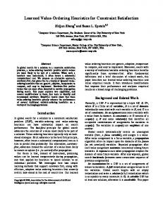
4.3.1.5 Lookahead Strategy The final aspect we can vary is our choice of lookahead strategy which defines the order in which we explore states. The entire search space of states is a tree containing a path from root to node for each combination of possible assignments to the unassigned variables of the QCSP. Our lookahead strategy defines an ordering in which to explore those states, and due to the time limit we will in general not explore the entire tree, but instead merely a sub-tree of it. Four different lookahead strategies were reviewed in section 2.4.5 and for convenience we describe them again here: Depth First (DF): Where one explores as far down each branch as possible before backtracking. Effectively exploring a path to each leaf node in turn. 105

Figure 4.2: Depth-First Tree Traversal Breadth First (BrF): Where all the children of the root are explored first, then all of their children next, and so on. Effectively exploring the entirety of successively deeper levels of the search tree in turn. Best First: Where when a node is explored, its children are evaluated according to some heuristic and added to a list of unexplored nodes, and the unexplored node from the list which currently has the highest estimation is picked next. Minimax with Alpha Beta Pruning (AB): which performs a depth first lookahead but uses minimax reasoning and alpha and beta bounds to prune away parts of the search tree. To help illustrate how these strategies work, we present sample trees and number the nodes in the order a particular strategy would explore them. Depth First, Breadth First and Best First ignore the quantification of variables. Figure 4.2 shows the order in which nodes are explored for Depth First. We see that it explores a path from the root to a leaf node, then backtracks and finds the next path to a leaf node and so on until all paths have been explored. Figure 4.3 shows a Breadth First exploration of the tree. We see that all nodes at each level of the tree are explored completely before moving on to the nodes of the next level. 106

Figure 4.3: Breadth-First Tree Traversal Figure 4.4 shows how the nodes are explored in a Best First strategy. The numbers in square brackets are the heuristic evaluations of the nodes. The first node we explore is the root, which has two children with evaluations 5 and 6, so we add them to our list giving us {6, 5}. We then take the highest evaluated node from the list, which is the node with evaluation 6, and then add it’s children to the list. The children have evaluations 8 and 4, and so the list becomes {8, 5, 4}. We next explore the node with evaluation 8 and add it’s two children to the list, giving us {5, 4, 3, 2}. Next we explore the node with evaluation 5, and so on, continuing until the time limit is reached or all nodes in the tree have been explored. Best First is not very suited to adversarial opponents however. The best move for an existential variable is the one which is most likely to lead to a solution. For the universal however, the best move would be one which causes a failure. The best move for the existential variable is thus what would be considered the worst if it had been a universally quantified variable, and vice versa. To overcome this we introduce a new lookahead strategy, called Partial Best First. Partial Best First (PBF): PBF behaves as best first for existential nodes, inserting the children into the ordered list in accordance with their evaluations. But when exploring a universal variable, the best child (lowest scored evaluation) will be immediately explored and the remaining children are added to the list after all of the unexplored existential nodes. 107

Figure 4.4: Best-First Tree Traversal Implementation : Maintain an list, L, of nodes ordered by their evaluations according to some heuristic. When exploring an existential node, evaluate the children and then add them to L. Then explore the highest ranked node in the list next. When exploring a universal node, evaluate the children and explore the worst ranked child next. Negate the evaluations for the other children and then add them to L.

Figure 4.5 shows the order we explore the same tree as was used to illustrate Best First when we are using Partial Best First. Initially we explore the root node, which is Universal so we immediately explore the best (lowest) evaluated child node and add the other child node to our list after negating it, thus the list of evaluations becomes {−6}. Then when exploring the 2nd node, we add the two children nodes to the list so the list becomes {10, 9, −6}. We then explore the node with the highest evaluation next, which is node 3 with the evaluation of 10. Since the 3rd node is also universal, we immediately explore node 4 which had

the evaluation 6, and add the other child’s evaluation to the list after negating it, which gives us the list {9, −6, −10}. Since node 4 has no children we do not add anything from it to the list, and then again we explore the highest evaluated node from the list, which is the one with evaluation 9. This continues until all nodes have been explored or time runs out. 108

Figure 4.5: Partial Best-First Tree Traversal The effectiveness of PBF will be strongly dependant on how accurate the evaluation of the heuristic is for the universal children. If it correctly identifies the choice the universal player is likely to make then it will perform well, but if it gets it wrong large sub-trees which are irrelevant will be explored and used for reasoning. Figure 4.6 shows how the Minimax with Alpha Beta pruning strategy prunes values from the search space. The order the nodes are explored in is omitted for clarity, but it is the same as for Depth-First. Unlike for Best First (and Partial Best First) all the nodes within the tree are not heuristically evaluated, only the leaf nodes are evaluated. These evaluations are propagated back up using Minimax reasoning as was described back in Section 4.3.1.2. The node A is pruned and does not need to be explored because the previous node explored (B) gave the evaluation of 4, which means that at node C the universal, picking the minimum value, can assign it a value of 4 or less (if further nodes were explored below it and found to give an evaluation below 4). However, at node E the existential can already pick a better value than 4: the value 5 from node D. Thus since we know the universal can force the evaluation of node C to be at most 4, the entire subtree is strictly worse than the subtree we already explored at node D, and so the remainder of the sub-tree rooted at C (in this case, merely the node A) need not be explored. Similarly, the node B and its sub-tree can be pruned too. Since node G already has an evaluation of at least 7 after exploring one branch below it, and the universal at the root will thus not pick it over the other explored branch 109

Figure 4.6: Alpha Beta Pruning Tree Traversal which has an evaluation of 5. We also seek to improve the performance of DF and AB by having them make more use of the information from the heuristics: Intelligent Depth First(IDF) : as DF, but where child nodes are ordered according to heuristics so that they end up being explored in order from best to worst. Intelligent Alpha Beta(IAB) : as AB, but with children order as in IDF. Implementation: If using a stack implementation, the children will be evaluated and then added to the stack in order from worst to best. Thus when popping off the stack they will be removed in order from best to worst. If using a recursive implementation, the children will be evaluated and then the calls to the recursive function will be made in order from the best child to the worst. In Figure 4.7 we show an Intelligent Depth First traversal of the tree. The root is a universal variable, so we explore the child with the lowest evaluation first. The second node is existential, so we explore the child with the highest evaluation first. The third node is universal again so we pick the node with lowest evaluation first, then explore the 4th node which has no children, so we backtrack to the 3rd node and explore it’s unexplored child with the lowest evaluation. The 5th node 110

Figure 4.7: Intelligent Depth-First Tree Traversal

also has no children, so we backtrack to the 3rd node, which has no remaining unexplored children causing us backtrack again to the 2nd node. At the 2nd node we then explore the highest evaluated unexplored node, and so on until the entire tree is explored or time runs out. Intelligent Alpha Beta explores nodes in the exact same manner as IDF, generating heuristic evaluations of all child nodes to order their exploration, but the alpha-beta pruning remains the same as for AB: the only heuristic evaluations used for performing pruning are those propagated up from leaf nodes using minimax reasoning. For AB and IAB, we do not let them search to the bottom of the tree as it is too time consuming and they would not finish within our time limits. Instead, we perform an iteratively deepening form of (I)AB which searches to a fixed depth limit and then increases that depth limit before performing (I)AB lookahead again. We continue until we have searched to the final variable (maximum depth) or we have run out of time. When we run out of time, the results of the last completed (I)AB lookahead are used to make our decision. In our tests we have set the initial depth limit to 2 and at each iteration we increase the depth limit by 1. Also, since the alpha beta pruning is fundamentally tied in with the use of minimax reasoning, we do not allow the use of Maximax or Weighted Estimates state evaluation reasoning with either AB or IAB. They always use minimax reasoning regardless of the type of opponent. 111

Algorithm 23: F indMove(P), returns an int 1: root ← current state of P 2: D ← ∅ 3: Add root to D 4: best value ← first value in domain of Firstuv(root) 5: while D is not empty AND TimeLimit has not been reached do 6: curr state ← remove next state from D 7: if curr state has unassigned variables then 8: prunePureValues(curr state) 9: for each value a in the domain of Firstuv(curr state), AND while TimeLimit has not been reached do 10: child state ← assignPropagateAndEstimate(curr state, a) 11: if getEstimate(child state) != DWO then 12: add child state to D 13: PropagateEvaluations( P,root, curr state) 14: best value ← getBestValue( root ) 15: return best value

4.3.1.6 Complete Approach We now show how all of these different aspects are integrated together in our algorithms to allow actors to perform lookahead reasoning on their current decision during its time limits. We present this as multiple different algorithms for each of the different lookahead strategies, which also invoke the chosen implementation of the other aspects (constraint propagation, state evaluation reasoning, etc.) at certain points. Algorithm 23 shows the general algorithm ”FindMove” used by the Depth First, Breadth First and Best First lookahead strategies when reasoning about moves within limited time. prunePureValues(): is a function which calculates the pure values for the first unassigned variable. If the variable is existential, if a pure value is found, all other values are removed from its domain. If the variable is universal and the opponent is adversarial, each pure value that is identified is pruned from the domain, so long as this will not reduce the size of the domain to 0. The behaviour for universal variables varies for the non-adversarial opponents, as previously described. 112

assignPropagateAndEstimate(): is a function to generate a child state from the curr state. It assigns the value a to the first unassigned variable in curr state, then propagates with the chosen constraint propagator. After propagating it evaluates the newly reached state to give it an estimated score, based on the chosen heuristic. If the assignment caused a failure, the child state receives a special score to indicate a DWO occurred. getBestValue(): is a function which returns the value that leads to the child state with the best estimate. FindMove works as follows. It initially adds the unexplored root state of the problem to data structure D. Then we continue to reason until we have no more unexplored states left (D is empty) or we have run out of time. While reasoning, we remove the next unexplored state (curr state) from D (line 6) and check that it is not a leaf node (i.e. there still exists unassigned variables, line 7). We prune pure values as appropriate (line 8) and then begin exploring the different possible assignments for the first unassigned variable in curr state (lines 9-12). We generate each of the child states of curr state, and then add them to D, if they do not contain failures. After each state is explored, we then propagate up the estimates from its children back to the root in line 13, and update the currently believed best move at line 14. Once we have either run out of time or finished exploring every state possible, we then return the best move possible (line 15). For Intelligent Depth First, we alter the above algorithm to generate all of the children before adding any of them to D. The children are then ordered based on the chosen heuristic before being added to D. Algorithm 24 shows the additional lines which must be added to Alg. 23, replacing lines 9-12 of the old algorithm, to implement the IDF lookahead strategy. We first perform propagation and get estimates for all of the possible child states, in lines 1+2. Then the child states are ordered based on their estimates depending on the quantifier of the variable. If the variable is universal they are ordered in descending order using the function orderDescending (line 4), and if the variable is existential they are ordered in ascending order of evaluation using the function orderAscending (line 6). The ordered child states are then added to the data structure D at lines 7-9. For a universal variable, the states are ordered in 113

Algorithm 24: ExploreIDFChildren 1: for each value a in the domain of Firstuv(curr state), AND while TimeLimit has not been reached do 2: child states[a] ← assignPropagateAndEstimate(curr state, a) 3: if getQuantifier( Firstuv(curr state) ) = ∀ then 4: child states ← orderDescending(child states) 5: else 6: child states ← orderAscending(child states) 7: for each state child state in child states, AND while TimeLimit has not been reached do 8: if getEstimate(child state) != DWO then 9: add child state to D

descending order, the final child added to D is the one with the lowest evaluation, and since the data structure used is a stack, it means this is the first value that will be popped off the stack. Similarly for existential variables, the child with the highest evaluation will be popped off the stack first. For Partial Best First more substantial changes are needed, to account for the different behaviour for differently quantified variables. We again use Algorithm 23 but replace lines 9-13 with a function call to ExplorePBFChildren(curr state), which we describe in Algorithm 25. In this case, D is an ordered list which holds pairs (state, estimate) and the list is ordered based on the values of ’estimate’. getQuantifier(): is a function which returns the quantifier of the passed variable. child states: is an array to store all child states. estimates: is an array to store all estimates for the child states. wipeoutOccurred: is a boolean variable used to store whether a DWO occurred or not. Default value is false. getBestEstimate(): is a function which returns the best estimate from a passed array of estimates negate(): is a function which returns the negation of the passed value. 114

Algorithm 25: ExplorePBFChildren(curr state) 1: if getQuantifier( Firstuv(curr state) ) = ∀ then 2: for each value a in the domain of Firstuv(curr state) AND while TimeLimit has not been reached do 3: child states[a] ← assignPropagateAndEstimate(curr state, a) 4: estimates[a] ← getEstimate(child states[a]) 5: if estimates[a] = DWO then 6: wipeoutOccurred ← true 7: if wipeoutOccurred = false then 8: for each value a in the domain of Firstuv(curr state) do 9: if child states[a] has unassigned variables then 10: if estimates[a] = getBestEstimate( estimates ) then 11: prunePureValues(child states[a]) 12: explorePBFChildren(child states[a]) 13: else 14: add the pair (child states[a], negate(estimates[a]) ) to D 15: else 16: for each value a in the domain of Firstuv(curr state) do 17: child state ← assignPropagateAndEstimate(curr state, a) 18: if getEstimate(child state) != DWO then 19: if child state has unassigned variables then 20: add the pair (child state, getEstimate(child state) ) to D 21: PropagateEvaluations( P,root, curr state)

In explorePBFChildren(), existential variables are still treated as before (lines 16-20) and after exploring we still propagate the estimates back up to the root (line 21). However, universal variables are treated differently. Firstly the estimates for all of the child states are calculated and stored (lines 2-4). If a failure occurs for any of the values we take note of it and do not further explore any of the states (lines 5-7). If no failure occurred, we will explore the best child (line 10) and the rest of the children are added to D (line 14). We negate their estimation for the purposes of their ordering in D, but the actual estimate stored in the state is not negated (i.e. the value for use with Minimax, Weighted Estimates or Maximax when propagating up to the root is not negated). While all the lookahead strategies so far support stopping at any time during search and then returning the best move found so far, for Alpha Beta this is not 115

supported. Since we perform iterative deepening, in which repeated searches of increasing depth are performed, we do not take the best move found so far during the current search, but instead we use the best move found by the most recently completed search. We assume that at least one AB search can be completed within the time limit. Our initial depth is set to 2, which we have found can always be completed long before any of the time limits used in our tests. For our implementation of AB and IAB we do not maintain a data structure D, but instead use recursive function calls, as it allows the alpha and beta bounds to be maintained more easily. The recursive calls explores node in the same order as maintaining a stack for Depth First would, minus the nodes that are pruned by the alpha and beta bounds. Algorithm 26 shows our implementation of this iterative deepening behaviour, while Alg. 27 shows the recursive function used to implement the alpha beta pruning. scores: is an array for storing the respective scores of each value assignment to the first unassigned variable. SOL: is a special score indicating that all variables have been assigned without conflict, i.e. a solution has been reached. It is the best possible result for an existential, and the worst possible for an adversarial universal. getBestMove() is a function which returns which value is the best move, based upon the score for each value within the passed array. Algorithm 26 the prunePureValues() function always performs as though the opponent is adversarial regardless of what it may actually be, removing pure values from the domain of universal variables, as AB’s reasoning is based on Minimax and so these pure values would be pruned by the alpha beta bounds anyway, since a pure universal value is strictly worse than any other choice for an adversarial opponent. The algorithm functions by performing an AB search up to the current depth limit for each of the possible values for the first unassigned variable at the root state (line 15). Special cases of failures (line 12) and solutions (line 17) do not need further searching. The scores resulting from each AB search are stored and then compared to deduce which move has the best overall score (line 19), this will only be performed if the AB searches were fully completed and not 116

Algorithm 26: F indMoveAB(P), returns an int 1: root ← current state of P 2: prunePureValues(root) 3: while curr depthLimit < maxDepth AND TimeLimit has not been reached do 4: Alpha = -∞ 5: Beta = ∞ 6: for each value a in the domain of Firstuv(root), AND while TimeLimit has not been reached do 7: child state ← assignPropagateAndEstimate(root, a) 8: if getEstimate(child state) = DWO then 9: if getQuantifier(Firstuv(root)) = ∀ then 10: return bestMove ← a 11: else 12: scores[a] ← DWO 13: else 14: if child state has unassigned variables then 15: scores[a] ← alphaBeta(child state, curr depthLimit, Alpha, Beta) 16: else 17: scores[a] ← SOL 18: if TimeLimit has not been reached then 19: bestMove ← getBestMove(scores) 20: curr depthLimit ← curr depthLimit+1 21: return bestMove interrupted due to the time limit. Then, as long as time remains and the entire problem has not been searched, the algorithm loops, to perform it all again, but at an increased depth limit. When restarting the search we also reset the Alpha and Beta bounds to their original values (lines 4+5). Once the time limit has been exceeded, or the entire problem has been searched, we then return the best move from the last completed AB search. depthOf() is a function which returns the depth of the passed variable. Algorithm 27 performs the recursive Alpha Beta lookahead. The base case is when the depth limit is reached (lines 1+2), in which case we return the heuristic estimate of the state. Otherwise, we perform an Alpha Beta search for each of the children of the first unassigned variable, and update the Alpha (lines 14+15) 117

Algorithm 27: alphaBeta(curr state, curr depthLimit, Alpha, Beta), returns an int 1: if depthOf (Firstuv(curr state)) = curr depthLimit then 2: return getEstimate(curr state) 3: prunePureValues(curr state) 4: if getQuantifier(Firstuv(curr state)) = ∃ then 5: for each value a in the domain of Firstuv(root), AND while TimeLimit has not been reached do 6: child state ← assignPropagateAndEstimate(curr state, a) 7: if getEstimate(child state) = DWO then 8: score ← DWO 9: else 10: if child state has unassigned variables then 11: score ← alphaBeta(child state, curr depthLimit, Alpha, Beta) 12: else 13: score ← SOL 14: if score > Alpha then 15: Alpha ← score 16: if Alpha ≥ Beta then 17: return Alpha 18: return Alpha 19: else 20: for each value a in the domain of Firstuv(root), AND while TimeLimit has not been reached do 21: child state ← assignPropagateAndEstimate(curr state, a) 22: if getEstimate(child state) = DWO then 23: score ← DWO 24: else 25: if child state has unassigned variables then 26: score ← alphaBeta(child state, curr depthLimit, Alpha, Beta) 27: else 28: score ← SOL 29: if score < Beta then 30: Beta ← score 31: if Alpha ≥ Beta then 32: return Beta 33: return Beta

or Beta (lines 28+29) bounds as appropriate depending on the quantifier of the 118

variable. If the update causes Alpha ≥ Beta (lines 16+30), then we have detected that an earlier explored decision renders the current search redundant, as a better choice for the existential or universal exists and thus this area of the tree will never be reached. We then return the Alpha or Beta bound as appropriate. For Intelligent Alpha Beta (IAB), we alter Algs. 26 and 27 so that in each instance where child states are explored, we instead generate heuristic estimates for all of the child states first. We then call alphaBeta() on the children in order of those estimates. Algorithm 28 shows the modified version of AB’s Alg. 26. Note that the order is done in the opposite order to how it was for IDF, since there is no stack push and pop operations this time, the states are instead handled directly in the order they were ordered in. The alphaBeta algorithm (Alg. 27) also must be modified for IAB. We replace lines 5+6 with the pseudocode shown in Algorithm 29. This orders the child states in descending order, so that the one with the highest evaluation is explored first. Lines 20+21 for the universal case must also be replaced with the same pseudocode, except the ordering function called is orderAscending instead of descending. We have now shown the algorithms for using each of the different types of lookahead strategy, enforcing constraint propagation and state evaluation reasoning, and what heuristics we are using to evaluate states. We now empirically evaluate the different possible combinations of the different implementations for these aspects.

4.4 Experiments We tested on randomly generated binary QCSPs with strictly alternating quantifiers, using the generator described in section 3.4 which prevents the flaws described in [62]. For each value of Q∃∃ we generated 50 random problems. We use the number of solutions achieved as a measure of how successful the actors are at reaching their objectives, considering any length of partial assignment that leads to a failure as an equally bad (or good, for an adversarial universal) non-solution. We tested on all possible combinations of lookahead strategy and heuristic state eval119

Algorithm 28: F indMoveIAB(P), returns an int 1: root ← current state of P 2: prunePureValues(root) 3: while curr depthLimit < maxDepth AND TimeLimit has not been reached do 4: Alpha = -∞ 5: Beta = ∞ 6: for each value a in the domain of Firstuv(root), AND while TimeLimit has not been reached do 7: child states[a] ← assignPropagateAndEstimate(root, a) 8: if getEstimate(child state) = DWO then 9: if getQuantifier(Firstuv(root)) = ∀ then 10: return bestMove ← a 11: if getQuantifier( Firstuv(root) ) = ∀ then 12: child states ← orderAscending(child states) 13: else 14: child states ← orderDecending(child states) 15: for each state child state in child states, AND while TimeLimit has not been reached do 16: if getEstimate(child state) != DWO then 17: if child state has unassigned variables then 18: scores[a] ← alphaBeta(child state, curr depthLimit, Alpha, Beta) 19: else 20: scores[a] ← SOL 21: if TimeLimit has not been reached then 22: bestMove ← getBestMove(scores) 23: curr depthLimit ← curr depthLimit+1 24: return bestMove Algorithm 29: 1: for each value a in the domain of Firstuv(curr state), AND while TimeLimit has not been reached do 2: child states[a] ← assignPropagateAndEstimate(curr state, a) 3: child states ← orderDescending(child states) 4: for each state child state in child states, AND while TimeLimit has not been reached do 5: continue to line 7 of algorithm alphaBeta

120

uation and in our graphs we include those combinations which performed worst and best for any plot point, and any others which gave interesting behaviour. The other combinations which have middling performance between the best and worst are omitted from our graphs. Both participants receive the same time limit per decision unless explicitly stated otherwise.

We implemented our system in Java. The existential and universal participants each maintain their own distinct copy of the QCSP problem and reason upon this model, so they are not aware of what reasoning their opponent performs. We ran all tests on a single PC with both the existential participant and the universal participant performing lookahead in parallel. Each participant is allocated an equal priority thread to perform its lookahead reasoning in, and the only communication between them is either to announce their decisions on what value to assign to the current variable, or to announce when a domain wipe out has been reached and the existential has failed. As a result the actual cpu time each receives per move is approximately half of the time limit, since they are sharing a single core. In our implementation, we store states (i.e. the values still contained in domains) as we explore them during lookahead, under the assumption that the time limit is short enough that we cannot run out of memory space during it. If the time limits are longer, less saving of states and more recomputing may be necessary.

We found FC to always give inferior results to MAC, and we show an example of this in Figure 4.8. The figure compares performance against an adversarial opponent, where all that is varied is which type of propagation the universal actor and existential actor are using. We can clearly see that if the opponent uses MAC, then using FC will greatly degrade our performance. This is because the reduced pruning of FC causes the heuristic evaluations of states to be less accurate and makes our decisions less informed. As such our best option is to always use MAC as the stronger propagation benefits us against adversarial opponents, and for making more informed decisions in general. While the figure only illustrates this for one particular lookahead setup (using Alpha Beta), our testing found FC to be inferior in all cases. 121

Constraint Propagation Comparison (All using Alpha Beta with timelimit) 50

40

Solutions

30

20

10 Existential FC vs Universal FC Existential FC vs Universal MAC Existential MAC vs Universal MAC 0 15

20

25

30 Qee

35

40

45

Figure 4.8: n = 20, b = 1, d = 8, p = 0.20, q∀∃ = 1/2, T imeLimit = 1000ms

4.4.1 Empirical Evaluation when the Universal Actor is Adversarial In our tests with an adversarial opponent, both participants use MAC for propagation. We have already explained why MAC is best for the existential, and for the universal it is used because it gives better performance than FC as the comparison showed. Our first tests are against a complete searching universal who is selecting values perfectly and will always cause a failure if the existential assigns any value which is not part of a winning strategy. Figure 4.9, shows the performance of the different lookahead methods against such a universal opponent, who is using a complete alpha beta pruning lookahead that searches to the end of the search tree with no time limit on 20 variable problems. The actual choice of lookahead strategy here for the universal is irrelevant, as any of our strategies will search the entire search space when there is no time limit and give the same results. Existential players are restricted to still have the same time limit for looking ahead during the universal player’s moves as they do on their own moves so that they cannot 122

Against Universal using Alpha Beta with no timelimit 50

40

Solutions

30

20

10

DF IDF PP PBF PP AB IAB Problems with a Winning Strategy

0 25

30

35 Qee

40

45

Figure 4.9: n = 20, b = 1, d = 8, p = 0.20, q∀∃ = 1/2, T imeLimit = 1000ms also perform a complete lookahead. The plot for the number of problems with a winning strategy is the optimal performance one could expect to achieve against this perfect opponent. None of our heuristic+lookahead combinations achieves this optimal and we would not expect them to against a perfect opponent, although PBF using the proportional promise of the DGP (PP) does manage to match it for some of the values of Q∃∃ . We observe that IAB performs more poorly than AB on these problems, as calculating the value ordering is wasting time for no gain in pruning of the search space, or possibly pruning even less. All remaining figures are against incomplete opponents who share the same time limit per decision as the existential player. Figure 4.10 shows our average performance against a universal opponent using depth-first lookahead, also on 20 variable problems. As we saw in Fig. 4.9, DF is a weak heuristic+lookahead combination, and so this universal opponent likely is performing poor decisions. We sometimes can achieve a solution even when the QCSP has no winning strategy against such a poor universal opponent. We also see that at Q∃∃ = 30 where the problems are more difficult, IAB is more 123

Against Universal using Depth First with timelimit 50

40

Solutions

30

20

10

DF IDF PP PBF PP AB IAB Problems with a Winning Strategy

0 25

30

35 Qee

40

45

Figure 4.10: n = 20, b = 1, d = 8, p = 0.20, q∀∃ = 1/2, T imeLimit = 1000ms effective than AB. Both figures 4.9 and 4.10 are on small problems, in which we can calculate winning strategies to the QCSP in reasonable time. We find that on these smaller easier problems, AB often outperforms IAB as there is not much scope to improve the amount of pruning done by AB and so the added value ordering’s overhead causes it to perform more poorly. PBF PP also performs very well on these smaller problems, but it has scaling issues on larger problems. Figure 4.11 is on 51 variable problems against a depth first opponent, and shows that PBF PP does not scale well at all. On the other hand, as the problem’s size and difficulty increases, IAB becomes an increasingly better choice. The amount of pruning possible is greatly increased by the value ordering and significantly deeper levels can be explored than that of AB without value ordering. We do not include the number of winning strategies in the graphs of these larger problems, as it was not possible to calculate them in reasonable time. Figure 4.12 is against a universal using IAB, again on 51 variable problems. We see that by altering the universal’s heuristic+lookahead combination we significantly increase its effectiveness at reaching its objective, to cause failures and 124

Against Universal using Depth First with timelimit 50

40

Solutions

30

20

10 DF IDF PP PBF PP AB IAB 0 70

75

80

85

90

95

Qee

Figure 4.11: n = 51, b = 1, d = 8, p = 0.20, q∀∃ = 1/2, T imeLimit = 1000ms prevent solutions, against all the strategies of the existential. As the universal opponent is improved, IAB for the existential still maintains its lead in performance.

4.4.2 Empirical Evaluation when the Universal Actor is Random We next investigate the effectiveness of our approach against a universal who is picking randomly from the point of view of the existential. The universal can have a hidden objective which is neither to cause a solution to be reached or a failure to occur, of which the existential is not explicitly aware. In our actual tests in this section, the universal is truly picking values randomly, following a uniform random distribution. For the tests against random opponents, we reduced the time limit to 500ms as it is significantly easier to do better against a non-adversarial opponent and a limit of 1000ms makes differences between the methods less visible. We also increase the number of test cases to 100 as a randomly choosing opponent introduces more variance into the results and a larger 125

Against Universal using Intelligent Alpha Beta with timelimit 50

40

Solutions

30

20

10 DF IDF PP PBF PP AB IAB 0 70

75

80

85

90

95

Qee

Figure 4.12: n = 51, b = 1, d = 8, p = 0.20, q∀∃ = 1/2, T imeLimit = 1000ms sample space reduces this variance. We compare the best results using Minimax to those using Weighted Estimates, to give an insight into the improvement WE provides. Heuristic+lookahead combinations not explicitly stated as using WE are using Minimax. Figure 4.13 shows our results with both participants using MAC. We see that those using WE achieve solutions significantly more often than the amount of problems which had a winning strategy. The version of AB shown in the tests for this section will give up when detecting that all values lead to a failure, while the version of IAB shown picks randomly amongst those values which do not immediately cause a failure. We see that this random selection give a large performance boost to IAB over AB as it gives up less frequently, and that IAB is even superior to the WE combinations for many values of Q∃∃ . Figure 4.14 shows the same tests but using EQAC instead for propagation for both actors. We observe moderate improvements to the performance of the lookahead methods using WE as we would expect when using a propagation algorithm which does not remove solutions against a non adversarial opponent. Minimax 126

Against Universal using Random, using MAC 100

80

Solutions

60

40

DF BF AB IAB BF PP WE PBF GM WE Problems with a Winning Strategy

20

0 15

20

25

30 Qee

35

40

45

Figure 4.13: n = 20, b = 1, d = 8, p = 0.20, q∀∃ = 1/2, T imeLimit = 500ms does not show gains from using EQAC, since it would dismiss as being poor any choices not pruned by EQAC which would have been pruned by MAC. IAB does not benefit from EQAC, because it is using Minimax reasoning which prevents any of the states explored by EQAC, that MAC would not explore, from having their evaluations reach the root. This is because at a universal variable, if one value is a failure, that value will always be the one returned by Minimax, regardless of if you performed more reasoning on the other values or not.

4.4.3 Empirical Evaluation when the Universal Actor is Benevolent Finally we investigate benevolent universals, who may have their own objective which they are seeking to maximise and as part of that they also require that a solution be reached. Similarly to the random universal experiments, again reduce the time limit to 500ms to make the difference in performance between different strategies more visible. We keep the number of test cases at each value of Q∃∃ at 127

Against Universal using Random, using EQAC 100

80

Solutions

60

40

DF BF AB IAB BF PP WE PBF GM WE Problems with a Winning Strategy

20

0 15

20

25

30 Qee

35

40

45

Figure 4.14: n = 20, b = 1, d = 8, p = 0.20, q∀∃ = 1/2, T imeLimit = 500ms 50, as for the adversarial tests. We use maximax (MM) reasoning to improve performance against benevolent opponents. Figure 4.15 shows results while using MAC propagation against a universal using breadth-first lookahead with maximax. We see that almost all lookahead methods using maximax perform very well, with no clearly discernable best method. Once again we achieve significantly more solutions than the number of problems which had a winning strategy. By swapping propagation to EQAC, as shown in Figure 4.16, we can get even larger amounts of solutions. All lookahead methods receive a large increase in number of solutions achieved, with BF using MM and IAB doing best at low and mid range values of Q∃∃ and IDF PP MM performing best at many high Q∃∃ values.

4.4.4 Experimental Summary We have shown that by altering lookahead strategy, constraint propagation and state evaluation reasoning we can provide varying performance for the actors, and 128

Against Universal using Breadth First with Maximax with timelimit, using MAC 50

40

Solutions

30

20

DF AB IAB BF MM PBF PP MM IDF PP MM Problems with a Winning Strategy

10

0 15

20

25

30 Qee

35

40

45

Figure 4.15: n = 20, b = 1, d = 8, p = 0.20, q∀∃ = 1/2, T imeLimit = 500ms Against Universal using Breadth First with Maximax with timelimit, using EQAC 50

40

Solutions

30

20

DF AB IAB BF MM PBF PP MM IDF PP MM Problems with a Winning Strategy

10

0 15

20

25

30 Qee

35

40

45

Figure 4.16: n = 20, b = 1, d = 8, p = 0.20, q∀∃ = 1/2, T imeLimit = 500ms 129

that good combinations of these perform consistently more effectively allowing the actors to reach their goals more often. In particular, shown that versus an adversarial opponent, using IAB is the most effective lookahead method for the existential on larger more difficult problems, where the additional value ordering over AB can have a large positive effect on the amount of pruning the alpha and beta bounds allow. On smaller problems we find PBF to be most effective for the existential, but have shown it to scale poorly as problem size is increased. It scales poorly as it bases its search around the heuristic evaluation of the ’best’ value for a universal variable. When the size of the problem is increased, the accuracy of the heuristic evaluations is reduced and PBF ends up exploring inaccurate choices more often, and bases its decisions upon them. We also showed that against non-adversarial opponents we can frequently expect to form a solution even when there is no winning strategy. Using appropriate reasoning like Weighted Estimates or Maximax improves our performance significantly, and synergises well with changing to a propagation algorithm (EQAC) that maximises pruning while not pruning any solutions from the QCSP.

4.5 Conclusions In this chapter, we have taken QCSPs as being a model of Online CSP, where a winning strategy to the QCSP defines a strategy to guarantee reaching a solution to the Online CSP. For the case of solving Realtime Online CSPs, in which we are limited in the time to make each decision, we have defined and explored the process of Realtime Online Solving of Quantified Constraint Satisfaction Problems. Realtime online solving of QCSPs is necessary when a problem imposes time restrictions on the decisions and does not afford us enough time to find a winning strategy to the entire QCSP. We have explored using an approach of game-tree search from A.I. Game Playing adversarial reasoning within our limited time, to help us reach solutions when performing realtime online solving of QCSPs. At each decision, we perform a lookahead search, using constraint propagation to prune the search space and different search strategies to decide which portion of the pruned search space to explore. We use ordering heuristic estimations to guide some of the search strategies, and to evaluate the quality of the explored 130

states. These evaluations are then propagated back up the search tree to the root, to let us decide which value to assign the current variable. Taking this approach, we have shown how different lookahead strategies and different means of propagating the results of lookahead search back to the root should be used depending on the opponent. We have shown the choice of constraint propagation to have an important impact on the performance of an actor. We introduced a new level of consistency, Existential Quantified Arc Consistency, specifically designed to not prune solutions from the QCSP, which is suitable when facing non-adversarial universal actors and showed the clear improvement to performance it affords us. We demonstrated the need for modifying heuristics to allow comparison between states at different depths of the search tree, and provided two possible modifications to Dynamic Geelen’s Promise which achieve this: the Geometric Mean, and the Proportional Promise. The aim of this chapter was to show that our approach of using value ordering heuristics in combination with A.I. game playing reasoning allows us, through use of effective combinations of constraint propagation, lookahead strategy and state evaluation reasoning, to improve the performance of the actors in a QCSP with limited time per decision. We have successfully shown that it can give good performance on a selection of randomly generated binary QCSP. On small problems, we have shown that we do not perform significantly worse than a complete search would when facing a perfect opponent, and that against a weaker opponent we can sometimes find solutions even when no winning strategy exists. We have modeled random QCSPs which are too large to solve and showed that realtime online solving of QCSP can be applied to them, reaching solutions interactively within short time limits. For non-adversarial opponents, we have shown impressive performance from the approach, managing to reach solutions far more often than winning strategies exist.

131

Chapter 5 Realtime Online Solving of QCSPs applied to Online Bin Packing 5.1 Introduction In this chapter, we apply Realtime Online Solving of QCSPs through Game-Tree Search to problems with structure and more complex constraints: variants of the Online Bin Packing problem, to show that the good performance seen in the previous chapter is not limited merely to randomly generated problems. We show that with good value ordering heuristic and lookahead combinations the approach improves the performance of the existential solving actor over that of an existential using a strategy like Best Fit without lookahead. It is necessary to show that the existential does well against strong adversarial opposition, so we also focus on improving the universal actor’s decisions and show that we can provide significantly stronger opponents than a strategy of Largest First without lookahead and that our existential actors perform better than Best Fit against these stronger universals. When modeling practical applications, the rules of the problem often require that illegal or invalid moves be pruned from the domains of universal variables as a result of earlier decisions, as previously described in Section 2.3.5. In Section 5.2 we introduce a system for modifying a model which was designed as if all the variables were existentially quantified, to introduce shadow variables where nec132

essary so that the model is valid when the quantifiers of the variables are correctly taken into account. This allows the universally quantified variables to represent ”for all legal moves” as opposed to ”for all moves”. Section 5.3 presents our models for two variants of online bin packing problems. We present the models initially ignoring the quantifiers and then provide the modified versions which includes shadow variables, following the previously described approach. The models use non-binary constraints and we present two useful new quantified non-binary consistencies, Existential Quantified Generalised Arc Consistency which is a a modification of SQGAC (reviewed in Section 5.4.2) and provides a reduced level of propagation but does not remove solutions, similar to EQAC for binary constraints which was introduced in Section 4.3.1.3, and also QnFC0 a quantified version of non-binary forward checking which performs a very weak level of consistency but is fast to maintain. Section 5.4.1 describes new heuristics designed for online bin packing problems based upon first fit and best fit. We experiment on small and larger problems and present the results in Section 5.5. Based on the initial results, we introduce a new heuristic, MinSpace, for the Type2 problems and show it to be significantly more effective choice for the universal than the other heuristics, and also much stronger in comparison with the Largest First strategy of picking values without lookahead.

5.2 Modeling with Shadow Variables As was previously discussed in Section 2.3.5, when attempting to model many ”natural” problems as QCSPs, a common issue occurs. Earlier choices can often preclude future choices, or choices may only be possible if a certain state has been reached. For example in the game of Chess, a pawn can only be moved to position e7 if it was already moved to e6 on an earlier move, or if it were already moved to d6 or f 6 and there is an opposing piece for it to capture at e7. If we are modeling the moves of one of the players as the universal variables of the problem, then the domain of those universal variables must include the value for moving the pawn to e7. But if the prerequisite moves have not yet been played the universal player should not be allowed to play the move at that turn. The rules of Chess require 133

that we prune these illegal moves from the domain of the universal for their next turn, but removing a value from the domain of a universal variable is considered a failure and causes a backtrack in QCSPs. In general, when modeling QCSPs, it is frequently found that a problem has similar rules requiring us to remove illegal choices from the domain of a universally quantified variable and they need to be removable without causing a backtrack. In order to overcome this issue the three different methods reviewed in Section 2.3.5 have been proposed, and in this section we provide an automated system for implementing Nightingale’s shadow variable approach[92] to pruning illegal values from universal variables. Since our solver implementation is based upon QCSP-Solve and supports pure value pruning, modeling the problem with shadow variables works naturally, but the value ordering and lookahead reasoning methods we use should work with an implementation based on QCSP+ too. We assume that a model containing constraints of arbitrary arity is created ignoring the pruning issues caused by the quantification of the variables and then show how to modify it to prune appropriately from the universal domains through exploitation of the pure value rule. This approach is suitable for modeling QCSPs in general, and not limited to modeling for realtime online solving of QCSPs.

5.2.1 Introducing Shadow Variables to a Model It is important to distinguish that there are two types of constraints that a universal variable can be a part of: those which are enforcing the rules of the game (what we shall call a rule-constraint), which results in the illegal moves we want to prune, and also those which are constraints of the problem (what we shall call a standardconstraint), where an invalid value should still cause a failure. It is assumed that the person modeling a problem has enough knowledge to identify to which of these types a constraint belongs. Only variables earlier in the variable sequence than the universal variable should be a part of a rule, as it is only earlier decisions that render moves legal or illegal. For every variable vi , where Qi = ∀ and there exists at least one rule-constraint over the variable vi , we introduce a new shadow variable ∃svj immediately after it in the variable sequence, with Dj = Di . We must then change all of the constraints that the variable vi was involved in. Note 134

that if no rule-constraints exist over a universal variable, a shadow variable should not be added for it, and the standard-constraints over it need not be altered. We initially give descriptions of how we modify the different possible types of constraints containing only a single universal variable. Then we show how to convert a constraint containing multiple universal variables into multiple constraints containing only single universal variables, upon which the previously mentioned modifications can then be applied. 5.2.1.1 Standard-Constraints If we have a standard-constraint C over the variables ∃x1 ..∃xn ∀v1 ∃xn+1 ..∃xm , where there may be 0 existential variables before or after the universal, then to modify C to work with shadow variables, we need merely replace the universal variable with the shadow variable. Thus this constraint is changed to be over the variables ∃x1 ..∃xn ∃sv1 ∃xn+1 ..∃xm . Algorithm 30 provides pseudocode for performing this operation when given a constraint Ck which contains the single universal variable v1 . For all these algorithms we assume that the shadow variable sv1 , which has a domain containing all the values in Dv1 , has already been added to the problem P. Algorithm 30: StandardConstraintSV(P, Ck ) 1: Create new constraint Cj over the variables ∃x1 ..∃xn ∃sv1 ∃xn+1 ..∃xm , with CjS = ∅ 2: for each value a ∈ Dv1 do 3: for each tuple t = (tx1 , .., txn , a, txn+1 , .., txm ) ∈ CkS do 4: CjS = CjS ∪ t 5: remove Ck from P 6: add Cj to P

5.2.1.2 Rule-Constraints If we have a rule-constraint R, over the variables VR = {x1 , .., xn , v1 } with quantifiers ∃x1 ..∃xn ∀v1 then we must convert it to a new constraint sR over the variables VsR = {x1 , .., xn , v1 , sv1 } with quantifiers ∃x1 ..∃xn ∀v1 ∃sv1 . We seek to make all 135

invalid universal values in R become pure values in the new constraint sR. Table 5.1 shows the truth table for an example rule-constraint R which states that variables x and y must take different values, where D(x) = D(y) = 0, 1, 2. Any tuple which is not valid, needs to cause that value of y to be pure in sR. Table 5.1: Constraint R ∃x ∀y Valid Tuple (a) 0 0 N (b) 0 1 Y (c) 0 2 Y (d) 1 0 Y (e) 1 1 N (f) 1 2 Y (g) 2 0 Y (h) 2 1 Y (i) 2 2 N Table 5.2 shows the tuples generated for sR from the tuple (a), a non-satisfying tuple, in R. For every value in the domain of sy the tuples will satisfy the new constraint sR. This means that once 0 has been assigned to x the value 0 becomes pure for y. Table 5.3 shows the tuples generated for sR from the tuple (b) which was a satisfying tuple in R. When the value of sy = y it is a satisfying tuple, for all other values of sy the tuples do not satisfy the constraint sR. This enforces the requirement that when we select a value for the universal y that the shadow variable sy will take the same value, which is necessary for the standard-constraints over sy to prune the universal as they were originally intended to. More formally, for each tuple t assigning values to variables VR of constraint R, there will be n tuples t′1 ..t′n where t′i |VR = t assigning values to variables VsR of constraint sR, where n is the size of the domain of the universal variable y. If t satisfies the constraint R, then t′i will satisfy the constraint sR if sy = y, otherwise it will not

satisfy it. If t does not satisfy the constraint R, then t′i will satisfy the constraint sR, for all i. For extensionally defined constraints, Algorithm 31 describes how to do this in pseudocode for a given rule constraint Ck over variables ∃x1 ..∃xn ∀v1 .

For intensionally defined constraints, if the constraint is defined by the expression expr, then the new constraint replacing it should state: (expr) ⇒ (sy = y). 136

Table 5.2: Tuple (a) added to constraint sR ∃x ∀y ∃sy Valid Tuple 0 0 0 Y 0 0 1 Y 0 0 2 Y Table 5.3: Tuple (b) added to constraint sR ∃x ∀y ∃sy Valid Tuple 0 1 0 N 0 1 1 Y 0 1 2 N Algorithm 31: RuleConstraintSV(P, Ck ) 1: Create new constraint Cj over the variables ∃x1 ..∃xn ∀v1 ∃sv1 , with CjS = ∅ 2: for each value a ∈ Dv1 do 3: for each tuple t = (tx1 , .., txn , a) ∈ Dx1 × .. × Dxn × {a} do 4: if t ∈ CkS then 5: CjS = CjS ∪ (tx1 , .., txn , a, a) 6: else 7: for each value b ∈ Dsv1 do 8: CjS = CjS ∪ (tx1 , .., txn , a, b) 9: remove Ck from P 10: add Cj to P If a standard constraint removes a value from the domain of sy, if that value is pure in y then it will remain pure as all the remaining values in the domain of sy are still supported. Thus a standard-constraint over sy will not interfere with the pure value functionality of the rule-constraint. If the value a ∈ Dsy removed from sy is not a pure value in y, then a ∈ Dy will lose its only support and be

pruned from the domain of y, causing a failure. Thus a rule-constraint maintains the desired functionality of the standard-constraints.

5.2.1.3 Multiple Rule-Constraints on the same Universal If we have multiple rule constraints over the same universal variable, it is necessary to combine them into one larger constraint. If we have two constraints R1 137

over the variables VR1 = {xa , .., xb , y} with quantifiers ∃xa ..xb ∀y and R2 over the variables VR2 = {xl , ..xm , y} with quantifiers∃xl ..xm ∀y and we must form a combined shadow rule-constraint sR1+2 over the variables VsR1+2 = VR1 ∪ VR2 ∪ sy with quantifiers ∃xa ..xb , xl ..xm ∀y∃sy to replace them. For every tuple t1 which does not satisfy the constraint R1 , in the combined shadow constraint sR1+2 any

tuple t′1 where t′1 |VR1 = t, will satisfy the constraint sR1+2 . Similarly for every tuple t2 which does not satisfy R2 , any tuple t′2 where t′2 |VR1 = t, will satisfy the

constraint sR1+2 . For all other tuples in sR1+2 , they will satisfy the constraint if and only if the value of y = sy.

In Algorithm 32 we show how two extensionally defined constraints Ck1 over variables Xk1 = {∃xi ..∃xn ∀v1 } and Ck2 over variables Xk2 = {∃xl ..∃xm ∀v1 } can be merged. The algorithm assumes a particular ordering (xi , ..xn , xl , ..xm , v1 ) for the variables but can easily be modified for whatever the actual ordering of the variables in the quantifier sequence may be. To improve legibility of the al-

gorithm, we denote as ×Xj the cartesian product of the domains of the set of variables Xj . For intensional constraints, if constraint R1 is defined by expr 1 and constraint R2 is defined by expr 2 , then the new constraint replacing them should state: ( expr 1 & expr 2 ) ⇒ (sy = y). Table 5.4 shows two sample constraints R1 and R2 over variables x1 , x2 and y with D(x1 ) = D(x2 ) = D(y) = 0, 1 and table 5.5 shows the combined constraint sR1+2 which replaces them.

5.2.1.4 Constraints which are both Rule and Standard When modeling a problem initially it can be convenient use a single global constraint to express both a rule (as we want it to prune illegal values from a universal variable) and a standard constraint (as it has more variables after the universal variable) at the same time. This is often the case for example when using an allDifferent constraint: We wish to enforce a rule on the decisions such that each choice cannot be the same as the ones preceding it, however the universal variable representing one decision is not the final variable/decision in the problem. These constraints, which both express a rule and a standard constraint, are just a shorthand used instead of describing the two constraints separately and we must extract 138

Algorithm 32: MultipleRuleConstraintSV(P, Ck1 , Ck2 ) 1: Create new constraint Cj over the variables Xj = {∃xi , ..∃xn , ∃xl , ..∃xm , ∀v1 , ∃sv1 } with CjS = ∅ 2: for each value a ∈ Dv1 do 3: for each tuple t1 = (txi , .., txn , a) ∈ Dxi × .. × Dxn × {a} do 4: if t1 ∈ CkS1 then 5: for each tuple t2 = (txi , .., txn , txl , .., txm , a, a) ∈ ×Xj where t2 |Xk1 = t1 do 6: CjS = CjS ∪ t2 7: else 8: for each value b ∈ Dsv1 do 9: for each tuple t2 = (txi , .., txn , txl , .., txm , a, b) ∈ ×Xj where t2 |Xk1 = t1 do 10: CjS = CjS ∪ t2 11: for each tuple t1 = (txl , .., txm , a) ∈ Dxl × .. × Dxm × {a} do 12: if t1 ∈ CkS2 then 13: for each tuple t2 = (txi , .., txn , txl , .., txm , a, a) ∈ ×Xj where t2 |Xk2 = t1 do 14: CjS = CjS ∪ t2 15: else 16: for each value b ∈ Dsv1 do 17: for each tuple t2 = (txi , .., txn , txl , .., txm , a, b) ∈ ×Xj where t2 |Xk1 = t1 do 18: CjS = CjS ∪ t2 19: remove Ck1 from P 20: remove Ck2 from P 21: add Cj to P the two constraint from them in order to create a correct shadow variable model. Any constraint with a single universal variable which is not the final variable is considered to be of this type. The automated system for splitting constraints with multiple universal variables (see Section 5.2.1.5) often generates constraints of this type which need to be processed. We take as an example an allDifferent constraint over variables ∃x∀y∃z. We must split the constraint into two constraints: the standard-constraint which contains all of the variables and is identical to the original constraint, and the ruleconstraint which includes the existential variables necessary for enforcing the rule 139

∃x1 0 0 1 1

∃x1 0 0 0 0 0 0 0 0

∃x2 0 0 0 0 1 1 1 1

∀y 0 0 1 1 0 0 1 1

Table 5.4: Constraints R1 and R2 R1 R2 ∀y Valid Tuple ∃x2 ∀y Valid Tuple 0 N 0 0 Y 1 Y 0 1 Y 0 Y 1 0 N 1 N 1 1 N

Table 5.5: Constraint sR1+2 ∃sy Valid Tuple ∃x1 ∃x2 ∀y 0 Y 1 0 0 1 Y 1 0 0 0 N 1 0 1 1 Y 1 0 1 0 Y 1 1 0 1 Y 1 1 0 0 Y 1 1 1 1 Y 1 1 1

∃sy 0 1 0 1 0 1 0 1

Valid Tuple Y N Y Y Y Y Y Y

(those preceding the universal variable), as well as the universal variable. In this case, the rule-constraint we need to extract, R1 , would be over the variables ∃x∀y.

A tuple t in the new rule-constraint satisfies the rule-constraint if in the original constraint there existed a satisfying tuple t′ , where t′ |VR1 = t, to the original constraint. If no such tuple exists, the tuple t in the new rule-constraint does not satisfy the constraint.

Algorithm 33 shows how we can generate the rule constraint from a constraint Ck which is both a standard-constraint and a rule-constraint. We assume Ck is over the variables Xk = {∃xl , .., ∃xm ∀v1 ∃xm+1 .., ∃xo } and that the existential variables involved in the rule-constraint part are {∃xl , .., ∃xm }. Extracting the rule-constraint from an intensionally defined constraint can be a non-trivial task and relies on thorough understanding of the rule the constraint was expressing. Once the rule-constraint is generated, it and the standard-constraint can both be processed as already described to generate appropriate shadow variable constraints. 140

Algorithm 33: ExtractRuleConstraint(P, Ck ), returns a constraint 1: Create new constraint Cj over the variables Xj = {∃xl ..∃xm ∀v1 }, with CjS = ∅ 2: for each tuple tj ∈ ×Xj do 3: for each tuple tk ∈ ×Xk where tk |Xj = tj do 4: if tk ∈ CkS then 5: CjS = CjS ∪ tj 6: return Cj

5.2.1.5 Constraints with multiple Universal Variables All of the types of constraints described so far have assumed that merely one universal variable is a part of the constraint. If we have multiple universal variables we need generate constraints with only 1 universal in them. We generate one new constraint for each of the universals in the original constraint. In these new constraints, they are still constrained by all of the same variables, with the exception that instead of being constrained by the other universals, they are constrained by their shadow variables instead. As an example, if we take a constraint C over the variables ∃x1 ∀y1 ∃x2 ∀y2 ∃x3 we replace it with two constraints C1 and

C2 . Where C1 is over the variables ∃x1 ∀y1 ∃x2 ∃sy2 ∃x3 and C2 is over the variables ∃x1 ∃sy1 ∃x2 ∀y2 ∃x3 , where sy1 and sy2 are the shadow variables of y1 and

y2 respectively.

Algorithm 34 shows how to convert a constraint Ck with at least 2 universal variables into multiple constraints with only one universal. The variables of the created constraints Cv are ordered such that if the shadow variables are replaced with their respective universal variables, they would then be identical to that of Xk . These newly created constraints are then processed as already described. However it is likely that a number of redundant identical shadow variable versions of standard-constraints are generated (in this example, 2 identical constraints over ∃x1 ∃sy1 ∃x2 ∃sy2 ∃x3 would be created) and only 1 of them need be retained. We also note that in the special case of all the variables of the original constraint being universally quantified, there is no need to retain any of the standard-constraints. The rule-constraints will render any value of universal yi as a pure value if the 141

Algorithm 34: ExtractSingleUniversalConstraints(P, Ck ), returns a set of constraints 1: constraints = ∅ 2: for each variable vi ∈ Xk do 3: Create new constraint Cv over the existential variables of Xk , vi , and the shadow variables of the universal variables of Xk , with CvS = ∅ 4: for each tuple t ∈ CkS do 5: CvS = CvS ∪ t 6: constraints = constraints ∪Cv 7: return constraints standard-constraints would prune that value from a shadow variable syi, so any pruning performed by the standard-constraints will have no effect on the decision variables (the universal variables). Following this system, any model with extensionally defined constraints can be converted into a shadow variable model suitable for QCSP. Intensionally defined constraints can also be converted, if the rule-constraints can be correctly extracted from the combination rule-standard constraints. The generated shadow variable model is valid, but it is not necessarily the only possible shadow variable model and other models may perform more or less efficiently than that created by this system.

5.3 Modeling Online Bin Packing We model two types of online bin packing problems, in which the universal actor is selecting the sizes of packets and the existential actor is choosing the bin in which to place the packet before the next packet arrives (i.e. is picked by the universal). The number of bins is fixed, and the existential succeeds (solves the QCSP) if all of the packets are successfully placed into the limited bins without overflow. The adversarial universal succeeds if the packets cannot be placed into the bins without overflow. The basic model is common to both problems and we describe it first, introducing shadow variables after first describing the model ignoring the modeling issues of the quantifiers. A known number of packets m will be chosen, and there 142

is a fixed number of bins k, each of the same capacity c. We use state variables for each bin to record how much capacity it has left, we have decision variables for the universal which determine the size of each packet, and decision variables for the existential to state the bin into which the current packet will be placed. As an example, the variables for the j th packet choice are ∃a(j−1)b1 , a(j−1)b2 , . . . , a(j−1)bk , ∀pj , ∃lj , a(j)b1 , a(j)b2 , . . . , a(j)bk where a(j−1)bi is the state of bin bi before the j th packet arrives, pj is the size of the j th packet, lj is the bin the j th packet is placed into, and a(j)bi is the state of bin bi after the j th packet has been placed. Each state variable a(j)bi stores the empty space left in a particular bin at that point. The following constraints for each j and i ensure the state variables are consistent: (lj = bi ) ⇒ (a(j)bi = a(j−1)bi − pj ) (lj 6= bi ) ⇒ (a(j)bi = a(j−1)bi ) When we introduce shadow variables after each universal variable, the variables for the j th packet choice become:

∃a(j−1)b1 , a(j−1)b2 , . . . , a(j−1)bk ∀pj ∃spj ∃lj a(j)b1 , a(j)b2 , . . . , a(j)bk spj is the existential shadow variable for universal variable pj . Since these constraints common to both models are standard-constraints, they are altered to act on the shadow variables instead of the universals as follows:

(lj = bi ) ⇒ (a(j)bi = a(j−1)bi − spj ) (lj 6= bi ) ⇒ (a(j)bi = a(j−1)bi ) We use the pure value rule to prune invalid values from the universal domains. While performing lookahead, we only check for pure values for the next unassigned variable. Our shadow variable model results in all constraints which con143

tain a universal variable having the universal variable as the second last variable, and its shadow as the final variable. Thus when checking whether a universal is a pure value, we are merely required to check if the value is supported by every value in the domain of the shadow variable or not. Since a universal value pruned as a pure value is an invalid value, according to the rules of the problem and as a result of the earlier made decisions, we make the alteration that if all universal values are pure we consider it as being a failure. To avoid the situation where valid universal values are pruned as pure values, we include a dummy value in the domains of the universal (and shadow) variables. This value is not pruned by any of the constraints in the problem, and so will always be present in the shadow variable’s domain and prevent a valid universal value being considered as pure. We use the value 0 for the online bin packing problems to serve this role, as the capacity constraints which ensure the state variables are consistent will always allow a packet of size 0 and never prune it. Thus, the domains of the universal variables are {0, 1, 2, .., c} in all problems.

5.3.1 Type-1 problems In the first type of online bin packing problems, the universal and existential players both share the same problem. The universal player has a fixed list of o packets of non-distinct sizes varying from 1 to c, with m as the total number of packets being provided and c is also the capacity of the bins. The list of packets for the universal is strictly larger than the number of packets it must pick, i.e. o > m, so it must choose both the sizes and ordering of packets to send. However, the subset of packets it can pick is restricted by an upper bound B on their combined size. For a problem with a given list of packets and upper bound B, by testing with a randomly picking universal and a strong adversarial universal we can evaluate the existential’s performance against approximations of both average case and worst-case order scenarios respectively. We can represent the fixed list of packets with a global cardinality constraint over the universal pj variables: gcc(p1, p2 , . . . , pm , vs1 , vs2 , . . . , vst ). 144

The domain for each pj is a set {s1 , s2 , ..., st } of possible sizes, and the vsi are variables, each of which has its own upper bound and a lower bound of 0. The constraint states that each value si must have cardinality of vsi in the set of values taken by the pj variables. E.g. if vs1 = {0, 1, 2} then 0, 1 or 2 of the pj variables may take the value s1 . The upper bound B on the combined sizes of the packets can be represented as a global sum constraint as follows: Σm j=1 pj ≤ B Combining the fixed list and the upper bound gives us the actual constraint for the Type-1 problems: gcc(p1, p2 , . . . , pm , vs1 , vs2 , . . . , vst ) AND Σm n=1 pn ≤ B In these type-1 problems, the universal has freedom as to what values to pick and in what order, and our aim is to show that by exploiting constraint propagation, lookahead and heuristics the universal can have a significant effect on the success rate of the existential, and similarly that the existential can perform better against a strong universal by also using those techniques. Before we can use the model we must first convert these constraints to shadow variable versions, to enable illegal values to be pruned from the universal domains. The gcc constraint, which is a rule-constraint over multiple universals, is first split into multiple gcc constraints, one for each universal variable pi constraining it with only the shadow variables of the other universal variables:

gcc(sp1 , sp2 , . . . , spi−1 , pi , spi+1 , . . . , spm , vs1 , vs2 , . . . , vst ) These are both standard-constraints and partially rule-constraints, so the ruleconstraints, which constrain the universal pi and the shadow variables of the universal variables before it in the quantification sequence, must be extracted. The standard-constraints are redundant and can be removed, as the rule-constraint for the final universal variable pm covers them. Then these gcc rule-constraints are 145

altered using the shadow variable of the universal to make the universal pure when values are illegal. Thus for each universal variable pi a shadow variable gcc ruleconstraint would look like:

(gcc(sp1, sp2 , . . . , spi−1 , pi , vs1 , vs2 , . . . , vst )) ⇒ (spi = pi ) Similarly, the global sum constraint is split, following the system previously provided, to sum constraints on each universal and the shadow variables of the universals before it.

((Σi−1 j=1 spj ) + pi ) ≤ B Since we know that the packets are a minimum of size 1 and that the sum of all of the packets is meant to be below or equal to B, we can slightly improve these sum constraints as below:

((Σi−1 j=1 spj ) + pi + |iuvpi |) ≤ B |iuvpi | is the number of inner universal variables pi has, i.e. the number of remaining packets after decision pi , which is a constant. We know that the sum of the earlier variables and the current universal variable and the inner universal variables must be far enough below B, and so |iuvpi | is the minimum possible sum of the sizes of the inner universal variables since they all must have a size of at least 1 each. Then adding in the universal’s shadow variable to allow pruning of illegal values, we end with the constraints of the form:

i−1 (((Σj=1 spj ) + pi + |iuvpi |) ≤ B) ⇒ (spi = pi )

Then the final form of the constraint for each universal pi , which contains both the list restriction and the upper bound restriction is as follows: 146

(gcc(sp1 , sp2 , . . . , spi−1 , pi , vs1 , vs2 , . . . , vst ) AND ((Σi−1 j=1 spj ) + pi + |iuvpi |) ≤ B) ⇒ (spi = pi ) While many efficient special purpose propagators for global constraints like gcc exist[70] in CSP, these propagators have yet to be extended to QCSP. As such, instead of making use of any special propagators for global constraints we use generic non-binary propagators like Nightingale’s SQGAC to propagate all constraints.

5.3.2 Type-2 problems The second type of online bin packing problems are designed to investigate the strength of our approach when the existential has an inferior view of the problem to the universal. The universal player has a fixed list of m packets of non-distinct sizes varying from 1 to c, where m is also the total number of packets being provided and c is the capacity of the bins, and must merely decide what order in which to provide the packets to the existential player. The existential player does not know the sizes of the packets before they arrive, but does know an upper bound on the total sum of all their sizes. Thus the existential is less informed than the universal and the two actors actually have slightly different synchronized problem models in which they reason and pick their values. For the universal’s view, we again represent the fixed list of packets with a global cardinality constraint over the universal pj variables: gcc(p1 , p2 , . . . , pm , cs1 , cs2 , . . . , cst ). The domain for each pj is a set {s1 , s2 , ..., st } of possible sizes, and the csi state exactly how many of the pj must take each value si . Note that the csi in this case are constants, rather than constrained variables, as we know the number of packets of each size present in the list, and all packets in the list must be used. The existential player does not see the gcc constraint; instead it sees a less restrictive 147

global sum constraint: Σm j=1 pj ≤ B where the variable B is defined as being B = Σtu=1 (su ∗ csu ), i.e. it is exactly equal to the sum of the sizes of the packets in the list. As for the Type-1 problems, we must introduce shadow variables, and the shadow variable rule-constraint form of the gcc constraint for each universal variable pi looks like:

(gcc(sp1, sp2 , . . . , spi−1 , pi , vs1 , vs2 , . . . , vst )) ⇒ (spi = pi )

Note that the vsi are variables, whose domains range from {0, 1, . . . , csi }, since we do not know the number of packets of each size that will have been chosen before each pi . This is an example of why extracting a rule-constraint from an intensionally expressed constraint which is both a standard-constraint and partially a rule-constraint can be non-trivial: if we had left the cardinalities as the constants csi instead of changing them to variables, then it would not perform correctly. For the existential’s view, the global sum constraint is split as shown previously for Type-1, giving us:

(((Σi−1 j=1 spj ) + pi + |iuvpi |) ≤ upperBound) ⇒ (spi = pi )

In the Type-2 problems, our aim is to show that the existential player can improve over strategies like First Fit or Best Fit, even when its perception of the problem is more restricted than that of the opponent. 148

5.4 Realtime Online Solving of Online Bin Packing QCSPs When realtime online solving these two variants of online bin packing QCSPs, we use the same lookahead strategies (DF, IDF, BrF, PBF, AB, IAB) and means of propagating estimates up the tree to the root (Minimax, Weighted Estimates) as on the randomly generated binary QCSPs in the previous chapter. However we introduce new heuristics specific to online bin packing problems and also new propagation, for non-binary constraints in general.

5.4.1 Heuristics for Online Bin Packing We developed two heuristics for online bin packing, based upon the principals of First Fit (FF) and Best Fit (BF). The Ordered Fitting (OF) heuristic is based on First Fit, and prefers states in which the first bin is the most filled, the second bin is the second most filled, etc.. For a problem with a set of k bins, b = {b1 , b2 , .., bk } of maximum capacity c, where fi is how full the ith bin is, we calculate OF as Σki=1 fi ∗ ck−i .

The Heavily Filled (HF) heuristic is based on Best Fit, and prefers states in which bins are as highly filled as possible and the rest empty, to those in which

many bins are only partially filled. We calculate HF as:

HF =

  1

for (fi ) = 0 (empty bin),

p  Σk fi /c for (fi ) > 0 i=1 The values of fi are calculated as follows: If the current first unassigned decision variable lj is existential, then the fullness of each bin fi can be calculated from c the initial capacity of each bin and a(j−1)b1 , .., a(j−1)bk the emptiness of each bin before placing the packet chosen at the previous universal decision. The heuristic then behaves as if the unplaced packet were put into the appropriate bin: the first bin with space for OF, and the best fitting bin for HF. That bin has its fi fullness increased as appropriate for if 149

Figure 5.1: Behaviour of Ordered Fitting (OF) the packet were placed inside it, and then the heuristic evaluates the entire state using the above formula. If the current first unassigned decision variable pj is universal, then the fullness of each bin fi can be calculated from c the initial capacity of each bin and a(j−1)b1 , .., a(j−1)bk the emptiness of each bin. The heuristic then evaluates the entire state using the above formula. As with the other heuristics used in Chapter 4, on an existential variable the highest evaluation is considered the best, while on a universal variable for an adversarial opponent the lowest evaluation would be considered the best. If no lookahead is performed, Ordered Fitting performs as First Fit, placing packets into the first bin they fit into, and Heavily Filled performs as Best Fit, placing into the fullest bin that can fit the packet. In Figure 5.1 we illustrate an example of how OF functions when it has deduced that a given stream of packets is incoming, assuming that it has performed a lookahead exploring all possible combinations of positions it could place those packets. If the lookahead only explored some of those states it may result in different decisions being made. In the initial state the first bin is 5/10ths full and the second bin is 6/10ths full. The lookahead has deduced that 3 packets of sizes 1,2 and 8 are coming. OF will 150

Figure 5.2: Behaviour of Heavily Filled (HF) attempt to maximise the fullness of the first bin before that of subsequent bins, so it places both the size-1 and the size-2 packet into the first bin, and then since the size-8 packet does not fit into either of the bins, it would have to place it into a third bin. For the same problem, Heavily Fitted performs quite differently as shown in Figure 5.2. HF prefers fuller bins, regardless of their order, and so the size-2 and size-8 packets would be placed into a third bin, to fill it perfectly. Then the size-1 packet is placed into the 2nd bin, since it is fuller than the first bin. Since the lookahead has predicted those 3 sizes of packet, their ordering does not matter as the heuristics will result in the same placement regardless. However if no lookahead were used, as for example with Best Fit, the ordering would affect their placement. If the order of packets arriving was 8, 2, 1 then BF would place them the same way as HF did in Figure 5.2. If however the ordering was 2, 1, 8 then BF would place them as in Figure 5.3. The first packet which is of size 2 would be placed into the second bin, as that is the fullest bin into which it can fit. Similarily, the second packet which is of size 1 would also be placed into the second bin. Then the third packet which is of size 8 would be placed into the third bin as it does not fit into either of the other bins. 151

Figure 5.3: Behaviour of Best Fit (BF) on the packet ordering 2, 1, 8

Thus, BF would be worse than HF for the ordering 2, 1, 8 since HF achieves a perfectly filled bin, which is optimal, while BF does not. But this is dependant on the lookahead allowing HF to deduce the packet sizes correctly which may not always be accurate. For this particular problem regardless of the ordering OF and First Fit would perform identically, but different packet orderings on other problems may result in different performance from the two similar to HF and BF. As with DGP in Section 4.3.1.1, we need to modify the heuristics to allow states at different depths of the search tree to be comparable. For these online bin packing heuristics, we use the Geometric Mean(GM) calculated as the nth root of the evaluation given by the heuristic, where n is the number of packets which have arrived. We also test using DGP and also the Proportional Promise (PP) and Geometric Mean (GM) modifications of DGP, in addition to the 2 new online bin packing heuristics. 152

5.4.2 Constraint Propagation for Non-Binary QCSPs We use three types of constraint propagation on the online bin packing problems: Strongly Quantified Generalised Arc Consistency (SQGAC), Existential Quantified Generalised Arc Consistency (EQGAC) and Quantified Non-binary Forward Checking 0 (QnFC0). SQGAC was defined by Nightingale[92] and we presented his algorithm for enforcing it in Section 2.3.2.1. EQGAC and QnFC0 are both new contributions of this thesis. For convenience the definition of SQGAC is reproduced here. Definition 5.4.1 (Strongly Quantified Generalised Arc Consistency (SQGAC)). M is a multiple winning strategy tree representing all the winning strategies W IN Pk for constraint Ck . Ck is SQGAC iff for each variable xki ∈ Xk and value a ∈ Dk , a vertex labeled xki 7→ a is contained in M. 5.4.2.1 Existential Quantified Generalised Arc Consistency SQGAC is a stronger level of consistency than GAC, ensuring that values which are not part of a winning strategy are pruned. However as we have seen for random binary problems in the previous chapter, retaining values which are part of solutions even if not part of a winning strategy can be desirable against non adversarial universal actors. Therefore, we define a new level of consistency, Existential Quantified Generalised Arc Consistency (EQGAC) for non-binary constraints which ensures existential variables’ values which are not part of a solution are pruned, whose implementation is based upon SQGAC-propagate. We define EQGAC as follows: Definition 5.4.2 (EQGAC (Variable)). A Variable xi is Existential Quantified Generalised Arc Consistent (EQGAC) if Qi = ∀, or if every value a ∈ Di is EQGAC consistent. Definition 5.4.3 (EQGAC (Value)). A value a in the domain of xi is Existential Quantified Generalised Arc Consistent (EQGAC) if Qi = ∀, or if for every constraint Ck for which xi ∈ Xk , there exists a tuple t ∈ CkS , s.t. each tuple element tj ∈ Dj and ti = a. 153

Definition 5.4.4 (EQGAC (Constraint)). A Constraint Ck is Existential Quantified Generalised Arc Consistent (EQGAC) if for every xi with Qi = ∃, where xi ∈ Xk , ∀a ∈ Di , ∃ a tuple t ∈ CkS , s.t. each tuple element tj ∈ Dj and ti = a.

Definition 5.4.5 (EQGAC (QCSP)). A QCSP P is Existential Quantified Generalised Arc Consistent (EQGAC) if every constraint Ck ∈ C is EQGAC consistent. All universal variables’ values are thus consistent, and a value for an existential variable is consistent if the value is part of a satisfying tuple for every constraint on that variable. Similarly to SQGAC, we maintain a tree Mk which is a multiple solution tree, representing all the solutions solPk for each constraint Ck . It is important to distinguish this from the ”solution trees” used by Verger and Bessi`ere [13], which were actually trees representing a winning strategy. A Multiple Solution Tree (MST) contains all solutions, even those not part of any winning strategy. Algorithm 35 gives a high level description of an algorithm for enforcing EQGAC consistency on arbitrary non-binary constraints: Algorithm 35: High Level Description of EQGAC-propagate(xki , a), returns a boolean 1: Consider MST = hV, E, r, Li : 2: (1) Remove all vertices labelled xki ← a from V and all edges including a vertex labelled xki ← a from E, and remove all subtrees which become disconnected from the root, r. 3: (2) Repeat the following to exhaustion: 4: Remove all vertices b with no children if b is not labelled with the final variable xkr . 5: (3) Any existential assignment no longer contained in the tree is pruned. If any domain is emptied, return false, otherwise return true. It has two important differences to SQGAC. Firstly, we only prune values from existential variables, the universal domains are never pruned by constraint propagation. Secondly, when a vertex representing an assignment to a universal variable is removed, we do not remove all of its siblings from the tree. These changes prevent the removal of solutions which are not part of a winning strategy. In SQGAC, such solutions get pruned because there exists a sibling of 154

one of the universal variable assignments in the solution, which is not supported (if no such unsupported sibling existed, that would make it part of a winning strategy). So by not pruning all children of a universal if one is unsupported, we can retain all the solutions which are not part of a winning strategy. And since the rest of the functionality of SQGAC is still present, we also retain all solutions which are part of a winning strategy too. We do not prune from universal domains which would cause a backtrack during lookahead search, since we are assuming we are facing non-adversarial opponents when we choose to use EQGAC propagation. Even if a value in a universal domain is not supported it can still be possible to reach a solution, as seen in the previous chapter using EQAC on binary QCSPs. We implement EQGAC-propagate using the same style of tree structure as Nightingale’s SQGAC-propagate. The vertices contain the same information as they did for SQGAC-propagate, and we also maintain a doubly linked list with headers for each assignment label. However removeVertex must be altered slightly to behave differently to maintain the MST. Universal values must never be pruned, as all are consistent according to the definition of EQGAC and Algorithm 36 shows the updated algorithm, which only adds existential assignments to the removeList. restoreVertex remains unchanged, as it does not cause any removals from domains. The concrete version of EQGAC-propagate is given in Algorithm 37. It performs as SQGAC, but does not prune all the siblings of a universal assignment if that assignment is pruned from the MST. In general, EQGAC performs less pruning than SQGAC, but it does not prune any solutions from the problem. This is a desirable property against non-adversarial universal actors, when performing realtime online solving of QCSPs. SQGAC applied to binary constraints is equivalent to AC for QCSPs[92], and EQGAC applied to binary constraints is equivalent to EQAC, since EQAC also never prunes universal values and only prunes existential values which are not supported by any values at all in some constraint, i.e. values which are not part of any solution to a constraint. In a standard QCSP solving performing top-down search, they are effectively performing a depth-first traversal of the search tree, and backtracking by restoring 155

Algorithm 36: (EQGAC) removeVertex(vertex : ver, inoutlist : removeList) 1: ver.p.cver.val ← nil {disconnect from the parent} 2: ver.p.nc ← ver.p.nc − 1 3: if ver.right = nil and ver.lef t = list(xver.var ← ver.val): then {ver is the last vertex with ver.var and ver.val} 4: if getQuantifier( ver.var ) = ∃ then {is not universal} 5: Add xver.var ← ver.val to removeList {therefore add to removeList} 6: if ver.right 6= nil then {disconnect ver from the list} 7: ver.right.lef t ← ver.lef t 8: if ver.lef t 6= nil then 9: ver.lef t.right ← ver.right 10: for all children ver.cj do {remove all children as well} 11: removeVertex(ver.cj ,removeList) Algorithm 37: EQGAC-propagate(xki , a), returns a boolean 1: removeList ← ∅ 2: for all ver ∈ list(xki ← a) do {iterate through the list} 3: while ver.p.nc = 1 or [∀(ver.var) and ver.val ∈ Dver.var ] : do 4: if ver.p.nc = 1 then {this vertex has no siblings 2} 5: ver ← ver.p 6: removeVertex(ver,removeList) 7: for all xkj ← b ∈ removeList do 8: if not exclude(xkj , b) then 9: return false 10: return true

the relevant vertices to the tree structure maintained by SQGAC and EQGAC effectively moves us back one level of the tree at a time. All movement between states is between directly connected nodes of the search tree. However, when performing lookahead game-tree search we are often not performing a depth-first search, and the next node chosen to explore may not be directly connected to the previous one. While we save the states of the domains of all variables at each explored node of the search tree, we cannot afford to do this for the tree structures maintained for every constraint by EQGAC and SQGAC, as they are time consuming to copy and too large to store. To overcome this, we save the 156

state of the tree structure at merely the root node of the current lookahead gametree, and repropagate decisions made to reach the new node we wish to explore. 5.4.2.2 Quantified Non-binary Forward Checking Both SQGAC and EQGAC require the creation and maintenance of a large tree data structure for each constraint in the problem. As problem size increases, the overhead of using these propagators rapidly increases. To combat this scaling issue, we introduce another new level of consistency which is low-cost to implement, though at the cost of providing very weak pruning. This new level of consistency which we call Quantified non-binary Forward Checking (QnFC0) is an extension of nFC0 [17], one of Bessi`ere et al.’s numerous versions of forward checking for non-binary CSPs. Definition 5.4.6 gives the definition of an algorithm to enforce nFC0. Definition 5.4.6 (Algorithm for enforcing nFC0). After assigning the current variable, apply arc consistency on all constraints involving the current variable and exactly one future variable. If the future variable’s domain is not emptied, continue with a new variable, otherwise backtrack. Extending the algorithm to enforce nFC0 to take account of quantifiers merely requires altering how we handle removals from the single future domain. If the domain is existential, proceed as with nFC0. If the domain is universal then we must backtrack. Modifying it thusly, we get we get an algorithm for maintaining Quantified nFC0 (QnFC0) which is defined in Definition 5.4.7: Definition 5.4.7 (Algorithm for enforcing QnFC0). After assigning the current variable, apply arc consistency on all constraints involving the current variable, past variables and exactly one future variable. If the future variable is existentially quantified, if the domain is not emptied, continue with a new variable, otherwise backtrack. If the future variable is universally quantified, if any value is removed from the domain, backtrack immediately, otherwise continue with a new variable. For our online bin packing problems and any models generated using our automated system to introduce shadow variables, QnFC0 shares EQGAC’s property 157

of not pruning any solutions. When we add in shadow variables, it means that every constraint still containing a universal variable will always contains its shadow variable immediately after it in the sequence as well. As a result of this, QnFC0 can only prune from existential domains and never from universal domains, and so, as with FC on binary QCSPs, it cannot prune away solutions. However, in general, the amount of values it does prune is significantly lower than those pruned by EQGAC.

5.5 Experimental Evaluation on Online Bin Packing Problems We now show the results of our tests on Online Bin Packing problems. We ran using the same system as for the random binary realtime online tests in Chapter 4. There are two notable differences compared to that system. Firstly, the two participants do not necessarily share exactly the same model, though decisions made by the participants in their model are always valid in the other’s model too. Secondly, the cost of maintaining copies of the SQGAC/EQGAC trees for all constraints at every search node during lookahead search is too high, both in terms of space to store them and time to copy them. As a result, we only store the states of the trees at the current root node of search, and re-calculate the state of the trees for each explored assignment to future variables. The state of the domains for each explored future state is still saved. We present results for 50 tests run at each upper bound on the total size of packets chosen by the universal. The lists of packets available for the universal to choose from are generated using a uniform random distribution. For Type1 problems we ensure that the sum of the generated list is exactly equal to the upper bound. For Type2 problems we only ensure that at least one combination of packets exists in the list which is below or equal to the upper bound. The number of packets is m, the number of bins is fixed k, and the capacity of bins/maximum packet size is c, where the domains of the universal variables are {0, 1, 2, .., c} for the pure value related reasons discussed earlier, even though actual packet sizes vary from 1 to c. The existential actor has a time limit per 158

decision of tl∃ milliseconds. The universal actor always has a 1000ms time limit. We consider it a success for the existential actor (and a failure for an adversarial universal actor) if all packets are successfully placed into the limited bins. If a packet cannot fit into any bin a domain wipe out occurs, and we consider it a failure for the existential actor (and a success for an adversarial universal actor). The variables storing the states of the bins are automatically assigned through propagation as a result of the universal’s decisions picking packet sizes, and the existential selecting which bin in which to place them. The actors do not get to spend any time performing lookahead before assigning these state variables their values. The actors only get time to perform lookahead search when assigning values to the decision variables: the universal variables for the selection of packet sizes, and the existential variables for selection of which bin in which to place them. In our graphs, we omit many of the lookahead+heuristic combinations for readability. In general, we show the best performing combination from each of 3 classes: Alpha Beta based lookaheads, combinations using Minimax and combinations using Weighted Estimates. As a baseline, we compared our existential actors against existentials using Best Fit and First Fit, which both perform no lookahead and place the current packet into the fullest bin which can fit it, or the first bin it can fit in respectively. As described in our review, Best Fit has very strong performance on the uniform average case of online bin packing problems[80], so matching its performance is our expected result when testing against a random universal actor. While against an adversarial universal, we expect to out perform BF, especially against stronger adversarials. The First Fit strategy is equivalent to picking the lexicographically first value for choice of bin which does not cause a failure if we apply constraint propagation after assigning it. We generally omit First Fit from the graphs, as it was strictly worse than Best Fit in all our test cases. Figure 5.4 shows a sample comparison of how the different constraint propagators perform in terms of solutions reached by the existential when facing the same universal. We can see that QnFC0 is worse, as expected, than SQGAC and EQGAC due to the reduced pruning it performs, and at times it is even worse than BF. This trend was present in all of our tests, although at times the performance 159

Propagation Comparison against an IAB FF Universal 50

40

30

20

10 IAB DGP (SQGAC) IDF DGP WE (EQGAC) IAB DGP (QnFC0) IDF DGP (QnFC0) BF 0 20

19.5

19

18.5

18 Upperbound

17.5

17

16.5

16

Figure 5.4: Type-2 problems: m = 4, k = 2, c = 10, tl∃ = 1000ms was a lot closer with QnFC0 almost equal to EQGAC or SQGAC. And so, on the smaller problems (4 and 5 packet problems, containing 22 and 33 variables respectively) in which using SQGAC and EQGAC is still viable, we will only show the results of SQGAC and EQGAC. On these problems for the existential actor, the Alpha Beta based lookaheads (AB and IAB) always use SQGAC. The lookahead+heuristic combinations using Minimax (MM) also use SQGAC, while the lookahead+heuristic combinations using Weighted Estimates (WE) use EQGAC. The universal actor always uses SQGAC propagation on the smaller problems. For the larger problems (10 packet problems, containing 96 variables) we use QnFC0 exclusively. As we raised the size of problems, the preprocessing time taken to generate the tree structures for SQGAC and EQGAC became progressively slower. When trying to generate problems with 5 packets and domains of size 11, the preprocessing time was already above 5 seconds while the time per decision is limited to 1 second, which meant that SQGAC/EQGAC were unsuitable for modeling such problems. For 10 packet problems the tree structures needing to be generated exceeded the runtime memory limits and could not be stored at 160

Against a Random Universal 50

40

Wins

30

20

10 IAB HF PBF GM-HF WE PBF GM-HF MM BF 0 20

19.5

19

18.5

18 Upperbound

17.5

17

16.5

16

Figure 5.5: Type-1 problems: m = 4, k = 2, c = 10, tl∃ = 1000ms all, rendering the use of SQGAC/EQGAC impossible. On the 4 and 5 packet problems, for our combinations using WE we use EQGAC propagation and for the combinations using MM or AB we use SQGAC propagation. In the 10 packet problems all combinations use QnFC0.

5.5.1 Type-1 Problems - Experimental Results We performed our testing on three sizes of problems: 4 packet problems with packet sizes varying from 1 to 10, 5 packet problems with packet sizes varying from 1 to 8, and 10 packet problems with packet sizes varying from 1 to 10. The number of packet sizes for 5 packet problems was reduced as SQGAC and EQGAC were too slow to preprocess 10 packet sizes. For all of the tests in this section, we generated a list of packets for the universal to choose from which was double the size of the number of packets to be chosen, i.e. list size = 2 × m. We first show our results on small problems against random universals. In Figure 5.5 which shows 4 packet problems, we can see that we achieve 161

Against a Random Universal 50

40

Wins

30

20

10 IAB OF PBF PP WE IDF DGP MM BF 0 24

23

22

21

20

19

Upperbound

Figure 5.6: Type-1 problems: m = 5, k = 3, c = 8, tl∃ = 1000ms a good improvement over BF for a number of upper bounds. On the 5 packet problems, shown in Figure 5.6 we see that we achieve less of an improvement, sometimes slipping below BF for the Alpha Beta and Minimax combinations, but the Weighted Estimates still perform well against BF, offering a small improvement for most upper bounds. Figure 5.7 shows our performance on larger 10 packet problems. While we do manage to perform as good as BF on a number of upper bounds, we do drop below too, most noticeably at upper bound 56. Comparing to FF, the WE and MM combinations perform as good or better than it for all upper bounds. So we are performing better than lexicographically picking, but not as well as the static heuristic BF does. In Figure 5.8, we show our performance on the same large 10 packet problems, but this with the existential being given 5 seconds per decision instead of 1. We see that the larger time limit does give some small improvements, at 3 different values of upperBound we see a small improvement over BF by different combinations, but still none of them is consistently better. If we could use a stronger 162

Against a Random Universal 50

40

Wins

30

20

10

AB OF IAB OF IDF GM-OF WE IDF GM-HF MM FF BF

0 60

59

58

57

56 55 Upperbound

54

53

52

51

Figure 5.7: Type-1 problems: m = 10, k = 6, c = 10, tl∃ = 1000ms consistency than QnFC0 we would likely match or surpass the performance of BF as we did at lower problem sizes, where SQGAC and EQGAC gave consistently better performance than BF, while QnFC0 was often only performing close to equal to BF. As work on efficiently solving QCSPs further advances we can expect the performance of our approach here to improve too. We now look at our performance on Type-1 problems against an adversarial opponent using IAB OF. Figures 5.9 and 5.10 show the results on small 4 and 5 packet problems. In both we can see consistent performance far above BF, especially at the higher upper bounds which are more difficult problems for the existential to win on. Again we scale up to larger 10 packet problems to confirm whether or not this good performance is maintained. However, as Figure 5.11 shows, the results are very surprising. We see a wide variety of results for different combinations. Some are barely beating the weaker First Fit strategy, while some like IAB HF are providing a strong improvement over BF at higher upper bounds though dropping at the lower upper bounds. The set of combinations using DGP (and PP variations of 163

Against a Random Universal 50

40

Wins

30

20

AB OF IAB OF DF DGP IDF GM-OF WE IDF GM-HF MM FF BF

10

0 60

59

58

57

56 55 Upperbound

54

53

52

51

Figure 5.8: Type-1 problems: m = 10, k = 6, c = 10, tl∃ = 5000ms Against an IAB OF Universal 50

40

Wins

30

20

10 AB HF IDF GM-OF PBF GM-OF WE PBF GM-OF MM BF 0 20

19.5

19

18.5

18

17.5

17

16.5

Upperbound

Figure 5.9: Type-1 problems: m = 4, k = 2, c = 10, tl∃ = 1000ms 164

16

Against an IAB OF Universal 50

40

Wins

30

20

IAB DGP IAB OF PBF PP WE PBF GM-HF WE PBF PP MM PBF GM-HF MM BF

10

0 24

23

22

21

20

19

Upperbound

Figure 5.10: Type-1 problems: m = 5, k = 3, c = 8, tl∃ = 1000ms it) are performing exceptionally well at all upper bounds. After further investigation, we deduced that the good behaviour of the DGP based combinations was due to them exploiting a flaw in the reasoning of an IAB OF universal actor. However we can still see that combinations like IAB HF still perform much better than BF on high upper bounds, even without exploiting the flaw. The IAB OF universal believes that the existential prefers situations in which the first bin is fullest, and so attempts to avoid that. In general, a 1000ms time limit allows approximately 3 ply of lookahead, if performing an alpha-beta lookahead. This is enough for the universal to estimate how the existential will decide to place the first packet and also to reason about what second packet it should send. After lookahead its likely decision is to pick a small item, say of size 3 with bins of capacity 10, which it expects the existential to place into the first bin. It can then follow this by placing a packet of size 8 which will not fit into the first bin and so the existential must place it in the second bin. This is ideal as the universal’s reasoning leads it to believe that having 4 or more in the first bin is better for the existential than having 3 or less and any amount in the later bins, due to how the 165

Against an IAB OF Universal 50

40

Wins

30

20

IAB DGP IAB HF PBF PP WE IDF GM-HF WE PBF PP MM IDF GM-HF MM FF BF

10

0 60

59

58

57

56 55 Upperbound

54

53

52

51

Figure 5.11: Type-1 problems: m = 10, k = 6, c = 10, tl∃ = 1000ms OF heuristic is calculated. However this reasoning proves faulty against the DGP based heuristics, as due to their particular implementation, they tend to put the first packet into the final bin instead of the first. After the first packet is placed into the final bin, the IAB OF universal again reaches the same conclusion, that the best thing to do is place a small packet into the first bin and then follow up with a large packet that will not fit into the first bin. As such, it continues to pick a stream of small packets until none remain and makes it very easy for the existential to place all packets into the bins. This shows why it is important that we identify strong universal actors to test against, as using IAB OF which is originally designed as an existential approach and performs well in that regard, is not necessarily a strong universal approach on these problems, even though it appears reasonably strong against BF. If we did not improve the universal actor’s performance, we would draw the conclusion that DGP combinations are always the best for Type-1 problems, which could prove to be a faulty conclusion. We focus on improving the universal in Section 5.5.3, 166

Against a Random Universal 50

40

Wins

30

20

10 IAB HF PBF PP WE PBF OF MM BF 0 20

19.5

19

18.5

18 Upperbound

17.5

17

16.5

16

Figure 5.12: Type-2 problems: m = 4, k = 2, c = 10, tl∃ = 1000ms after first looking at our initial performance in Type-2 problems.

5.5.2 Type-2 Problems - Experimental Results We now show our results for the Type-2 problems, in which the universal has a complete view of the problem, while the existential is reasoning in an inaccurate problem model where it does not know the actual possible packet sizes and merely knows their upperbound. We begin again by showing our results on the smaller 4 and 5 packet problems, with Figures 5.12 and 5.13 showing our performance against a universal actor using random selection. We see a consistent good performance compared to Best Fit in the 4 packet 2 bin problems. All of the heuristics are equal or better than BF for all upper bounds, with the Weighted Estimate combination slightly better at the highest bound, and the Minimax combination the weakest. However as we scale up the problem size to 5 packets with 3 bins, we see that we do not maintain this good performance. Some of the heuristics do worse than BF at many upper bounds. It 167

Against a Random Universal 50

40

Wins

30

20

10 IAB OF PBF PP WE IDF GM-HF MM BF 0 24

23

22

21

20

19

Upperbound

Figure 5.13: Type-2 problems: m = 5, k = 3, c = 8, tl∃ = 1000ms appears likely that our approach is not an improvement over BF as we scale up to larger problems, when facing a random opponent. However, as shown by Figures 5.14 and 5.15, against an adversarial opponent using IAB OF our approach seems quite effective, even as we scale up to the 5 packet problems, giving large consistent improvements over BF at the different upper bounds. We note that even though the opponent is adversarial, the WE combinations sometimes perform better than MM combinations. This is not an indication that the universal is weak (as we shall demonstrate later, it is not), but rather that many of the failures detected by the existential while looking ahead are not actually possible. The Type-2 problems have different models for the existential and universal actors. The universal has what can be viewed as the complete problem, while the existential has merely an approximation (knowledge of the upperbound) of the total problem. As a result, while looking ahead the existential’s heuristic evaluations may make incorrect conclusions of the existence of domain wipe outs or failures, based on the belief that the universal can play any combination of packets summing to the upper bound, when in fact the universal is 168

Against an IAB FF Universal 50

40

Wins

30

20

10 IAB HF IDF DGP WE PBF FF MM BF 0 20

19.5

19

18.5

18 Upperbound

17.5

17

16.5

16

Figure 5.14: Type-2 problems: m = 4, k = 2, c = 10, tl∃ = 1000ms more limited in its choice of sizes. These incorrect conclusions are propagated up by Minimax reasoning, believing them to be the move which the universal would select and that results in the poorer decisions compared to Weighted Estimates, which also propagates them up, but does not eliminate solutions while doing so. We continue to scale up these problems to larger problems to confirm if this behaviour continues or not, moving up to 10 packet problems again, which still requires the use of QnFC0 propagation exclusively. As already seen, QnFC0 propagation performs worse than SQGAC and EQGAC but we are hopeful that it can still maintain some lead over BF on large problems. Figure 5.16 shows our performance against a random universal actor. We still perform worse than BF, confirming that we cannot compete on these types of problems with BF, merely matching it at best for most upper bounds, if the universal actor is picking randomly. On these problems the lookahead can no longer explore a large proportion of the search space, and so our reasoning is much less informed, especially at the earliest decisions. Figure 5.17 shows our results against an adversarial universal actor using IAB 169

Against an IAB FF Universal 50

40

Wins

30

20

10 IAB DGP PBF GM-HF WE IDF DGP MM BF 0 24

23

22

21

20

19

Upperbound

Figure 5.15: Type-2 problems: m = 5, k = 3, c = 8, tl∃ = 1000ms Against a Random Universal 50

40

Wins

30

20

10 IAB OF IDF GM-OF WE IDF GM-HF MM BF 0 60

59

58

57

56

55

54

53

52

Upperbound

Figure 5.16: Type-2 problems: m = 10, k = 6, c = 10, tl∃ = 1000ms 170

51

Against an IAB OF 50

40

Wins

30

20

10 IAB OF IDF GM-HF WE IDF GM-OF MM BF 0 60

59

58

57

56 55 Upperbound

54

53

52

51

Figure 5.17: Type-2 problems: m = 10, k = 6, c = 10, tl∃ = 1000ms

OF, on large 10 packet problems. We see that even against an adversarial opponent, we cannot perform as well as BF on large problems, in fact we perform significantly worse than it for many upper bounds. The use of QnFC0 propagation hurts our performance, as we saw back in Figure 5.4 where we compared its performance to SQGAC and EQGAC. Even on smaller problems using QnFC0 was observed to sometimes give performance slightly below that of BF. Also, since the existential has a worse model of problem, the effects of the errors in its reasoning become more widespread when a smaller proportion of the problem can be searched during the time limit. Even when we increased the time limit to 5000ms for the existential the lookahead+heuristic combinations were still far below BF. Unfortunately, we must draw the conclusion that if the existential has an incorrect or vague model of the problem and is using weak constraint propagation, our approach can result in quite poor performance and should likely not be adopted. 171

5.5.3 Improving the Universal Actor We developed a new heuristic to improve the universal actor called, MinSpace(MS) when used by a universal, or Max Space when used by an existential, which does not suffer from the same flaw as OF.The principal behind MS is as follows: For the existential using this heuristic, it prefers states in which many bins are exactly full, and all others are as close to empty as possible, i.e. maximising the space in the bins. Since an adversarial universal prefers the states which an existential rates lowly, the universal using this heuristic will prefer states in which few bins are perfectly filled, and all others are very nearly full, i.e. minimising the space in the bins. This strategy of leaving only small spaces free in bins is intended to make it tough for the existential to fit everything into the bins when the upper bound is high and close to the total capacity of all bins. We calculate the MS measure using:

Σki=1

  1

for (c − fi ) = 0,

p   (c − fi )/c

for (c − fi ) > 0

Full bins get a maximal score when calculating MS, while partially filled bins get a higher score the less full they are. We also provide a strategy which does not perform lookahead, Largest First(LF) as a baseline to compare our lookahead and heuristic combinations against. Largest First follows the policy of picking the largest packet it can at each decision. Largest First is a rather naive policy and we expect our combinations for the universal actor to out perform it significantly, since these bin packing problems favour an intelligent universal. Picking the largest packets first generally limits the options of the existential, as a packet with size more than c/2 will always require a new bin to place it into. As a result, all heuristics are forced to perform identically until no more packets that large exist for the universal to pick. At this point, there is still a lot of restriction of choice due to the bins being mostly full and the remaining packets only fitting into some of them, as the largest packets possible continue 172

Against a BF Existential 50

40

Wins

30

20

10

BrF 1ply MS BrF 2ply MS IAB MS LF Random IAB OF

0 60

59

58

57

56 55 Upperbound

54

53

52

51

Figure 5.18: Type-1 problems: m = 10, k = 6, c = 10, tl∃ = 1000ms to be chosen. Empirically, we found that all our combinations and BF perform identically at all upper bounds against Largest First on both Type-1 and Type-2 large problems. In Figure 5.18 we show an existential using Best Fit for 10 packet Type-1 problems and compare its performance against different types of universals. We test against LF, IAB OF, IAB MS and also Breadth First(BrF) MS, which we limit to either 1 ply or 2 ply depth of lookahead to provide comparison between different strengths of MS reasoning. Since we are seeking to compare the strength of the universal, the plots which are lowest on the graph are the most effective as they allow the existential to win less frequently. We see that IAB MS is a significantly stronger opponent than LF and IAB OF. Note that simply doing a breadth first exploration to depth 2 using MS is very strong. Interestingly, we note that MS with an exploration of depth 1 ply performs dreadfully, as the reasoning behind it requires that lookahead be performed: it cannot be achieved as a static evaluation of a state. We now test on Type-2 problems, comparing universals using IAB OF and 173

Against a BF Existential 50

40

Wins

30

20

10 IAB MS LF Random IAB OF 0 60

59

58

57

56 55 Upperbound

54

53

52

51

Figure 5.19: Type-2 problems: m = 10, k = 6, c = 10, tl∃ = 1000ms IAB MS to LF and a random universal, to evaluate whether or not we are providing a suitably challenging universal opponent on those problems too. Figure 5.19 shows the comparison of an existential using BF to the various universals on 10 packet Type-2 problems. We see that IAB MS performs very closely to Largest First, giving small improvements at a few upper bounds. Since the main aim of the MS heuristic is picking good sizes of packets, it does not perform very well on Type-2 problems, where the sizes of packets are fixed and only their ordering can be altered. On the other hand, IAB OF does not suffer from the same exploitable flaw, as the choice of packets is fixed so it cannot pick more small packets than it should, as it sometimes does in the Type-1 problems. Thus we can see that IAB OF is a strong universal for Type-2 problems, as previously mentioned.

5.5.4 Testing Against a MinSpace Universal We now show the performance of different existential combinations against an opponent using IAB MS. On Type-2 problems, shown in Figure 5.20, we can see 174

Against an IAB MS Universal 50

40

Wins

30

20

AB OF IAB DGP DF DGP WE IDF GM-OF WE IDF GM-MS WE IDF GM-OF MM IDF MS MM BF

10

0 60

59

58

57

56 55 Upperbound

54

53

52

51

Figure 5.20: Type-1 problems: m = 10, k = 6, c = 10, tl∃ = 1000ms that most combinations are equal or slightly below BF at higher upper bounds, and some are slightly better at lower upper bounds. However, when we increase the time limit for the existential’s lookahead as in Figure 5.21, we can see a very large improvement in performance over BF. While there is a lot of variance between the combinations, we can see that at high upper bounds we can achieve very large improvements over BF with many combinations. And that most of the combinations continue to provide improved performance for all of the upper bounds, with DF MS WE in particular providing extremely good performance across the middle and low upper bounds. In general, for an Alpha Beta based lookahead, a time limit of 1000ms allows it to explore on average a depth of up to 3 ply. Increasing the time limit to 5000ms on average allows an increased depth of an addition 2 ply, or up to 5 ply total. Exploring 2 ply deeper means taking account of one more pair of packet size selection and placement decisions (or possibly a placement decision and then another packet size selection). By merely taking account of one more packet (in the case of AB, for Depth First or Partial Best First heuristics the additional ex175

Against an IAB MS Universal 50

40

Wins

30

20

AB MS AB OF IAB OF PBF PP WE DF MS WE PBF PP MM BF

10

0 60

59

58

57

56 55 Upperbound

54

53

52

51

Figure 5.21: Type-1 problems: m = 10, k = 6, c = 10, tl∃ = 5000ms plored space is more abstract), we can achieve such large gains over BF even on these larger problems.

5.6 Conclusions In this chapter we have explored the application of Realtime Online Solving of QCSPs through Game-tree Search to a more practical application: Online Bin Packing. We have shown that on smaller problems, in which we can utilise more powerful propagation algorithms, we can achieve very good results and outperform Best Fit, the best uniform average case online bin packing algorithm. For the Type-1 problems, in which the existential has the complete model of the problem, we have seen that when the problem size is increased our performance drops slightly below Best Fit against a random universal actor, due to the poorer level of constraint propagation we can enforce. However as QCSP propagation is improved and made more efficient to maintain, we can expect our perfor176

mance to raise. Against adversarial universal actors on Type-2 problems, we have shown that when a suitable amount of lookahead time is provided, our approach can achieve very large improvements over Best Fit even against the strongest of universal actors. For the Type-2 problems, in which the existential has a limited model of the problem, we have seen that as the problem size is increased, the weaker constraint propagation and the reasoning from lookahead can lead us to inaccurate decisions, which result in poor performance against both random and adversarial universal actors. We have also shown that our approach can be used to generate very strong universal actors. This is necessary for showing that our existential decision makers are effective even against difficult adversaries. For Online Bin Packing we take the adversarial universal as being an approximation of worst case performance, but in other applications of realtime online solving of QCSPs, it may be the case that the universal’s role and decisions are symmetrical to the existential’s e.g. such as in the game of chess. In this case, being able to generate a strong adversarial universal actor could result in the creation of a strong existential actor.

177

Chapter 6 Conclusions and Future Work 6.1 Conclusions The thesis defended in this dissertation is that: Value Ordering can enhance Quantified Constraint Satisfaction Problem solving. In particular: 1. when solving an entire QCSP, effective value ordering improves the efficiency of the search. 2. when reasoning on QCSPs interactively under time constraints, value ordering in combination with AI Game Playing adversarial reasoning allows the participants to achieve their objectives more frequently. In Chapter 3 we focused on solving entire QCSPs and applied value ordering heuristics to improve search. We considered two approaches to value ordering heuristic for QCSP. The first approach was Solution-Focused Adversarial, aiming to choose values based on whether or not they lead to a solution and was inspired by adversarial search. On existential variables we preferred values that maximise the chances of reaching a solution, while on universal variables we preferred values that minimise the chances of reaching a solution. The second approach was Verification-Focused, aiming to pick values which can quickly be verified as leading to a solution or not. We experimentally tested both approaches and showed classes of problems which each is suited to. We observed improvements in search 178

speed approaching an order of magnitude on some problems, conclusively showing that value ordering heuristics can improve the efficiency of search in QCSPs. In Chapter 4 we took QCSP as being a model for online CSPs, where a winning strategy to the QCSP guarantees we can reach a solution in the online CSP. We then looked at realtime online CSPs, in which we were limited in time per decision and did not have enough time to fully solve the equivalent QCSP before some decisions had to be made. Our approach was to use value ordering heuristics and AI game playing adversarial reasoning to reach solutions in the QCSPs. In this approach, which we called Realtime Online Solving of QCSPs Through Game Tree Search, we assumed two actors in the problem, one controlling assignments to the existential variables and the other the universal variables, and that each decision has a time limit. During that time limit the actors reasoned about what value to assign the current variable, taking account of the likely behaviour of the other actor. The actors performed a lookahead like in game tree search, exploring the possible future states that could be reached depending on the decisions made by both of the actors and using constraint propagation to reduce the size of the total search space. Value ordering heuristics were used to compare between states, and the results were propagated back up the search tree from the leaf nodes to the root. The values propagated up to the root were then used to decide which value to assign to the current variable. We empirically tested this approach on randomly generated binary QCSPs and showed that the approach was promising. It allowed us to reach solutions on problems which had no winning strategy for the QCSP, when facing non-adversarial universal actors (and also weak adversarial actors). Against strong adversarial universal actors we showed that the number of times we reached solutions was still close to the number of problems that had a winning strategy. We also tested on large problems which were infeasible to solve fully, and showed that the approach can be applied to reach solutions on these problems. In Chapter 5 we presented our automated system for introducing Nightingale’s shadow variables into models generated while treating all of the variables as if they were existentially quantified. The introduction of the shadow variables enables pruning from the universal domains within these models, overcoming the primary limitation of standard modeling in QCSPs. We modeled Online Bin Packing Prob179

lems in this manner and applied our approach of realtime online solving of QCSPs through game tree search to solving them, comparing our performance to that of Best Fit, an algorithm for bin packing with good worst case performance and the best uniform average case performance. We showed that on smaller problems, in which we have time to explore a significant proportion of the search space, we can out perform Best Fit against both adversarial and random universal actors, allowing the existential actor to reach solutions more frequently, if we use strong constraint propagation in the form of SQGAC and EQGAC. On larger problems we showed that our approach is not very effective in helping the existential actor when the existential’s view of the problem is a relaxed version of the true model. On larger problems where the existential’s view is identical to the universal’s, we saw performance drops slightly when using weaker constraint propagation (QnFC0) and facing a random universal actor, only managing to perform close to as good as Best Fit. However against strong adversarial opponents we achieved significant performance improvements for the existential actor over Best Fit, especially at the highest upper bounds on the total packet size, in which reaching solutions was most difficult. We also focused on improving the universal actor’s performance through use of superior value ordering heuristics, since a strong universal is necessary to validate the strength of the existential actor, and because in many problems a strategy that leads to a strong universal could potentially be adapted into being a strategy that gives a strong existential if the type of decisions they are making are the same. We introduced a new heuristic, called MinSpace, which gave significant improvements to the universal’s performance on the Type-2 class of problems. We compared our heuristics to the naive Largest First algorithm which picks the largest packet size to send next at each decision, and showed we can significantly outperform it, reducing the number of solutions all types of existential actor could achieve by a large margin. We also showed that the MinSpace heuristic on its own applied to the current state is not enough to achieve this performance, in Figure 5.18. The heuristic requires game tree lookahead to be able to perform well, it cannot be statically calculated without any lookahead. Chapter 5 provided a proof of concept of our approach for realtime online solving of QCSPs. It provides empirical evidence that supports our claim that 180

when reasoning on QCSPs interactively under time constraints, value ordering in combination with AI Game Playing adversarial reasoning allows the participants to achieve their objectives more frequently.

6.2 Future Work In our work on Value Ordering Heuristics for solving QCSPs, we found that heuristics need to balance two properties to be effective for QCSP solving in general: they must be solution-focused, aiming to select values which are part of a winning strategy, and they must be verification-focused, picking values which take the least effort to verify whether or not they are a part of a winning strategy. The example heuristics we explored fell into one of these two categories but it is possible for a heuristic to have both properties. The heuristic used by BlockSolve[13] is an example of a heuristic which has both properties: when assigning values to the current block, it tries to pick an assignment which is compatible with the most tuples for the outer blocks. Since this assignment is compatible with many outer tuples it is probabilistically more likely to be part of a winning strategy than an assignment which would only be compatible with one or two, and it also reduces the amount of branches it needs to explore up the tree from that block, thus allowing for faster verification. Finding a general heuristic for top-down QCSP solving which is both solution-focused and verification-focused may similarly be possible. It also remains to be investigated as to whether or not effective variable ordering for QCSPs, which is limited to within blocks of variables with the same quantifier, would also be required to be both solution-focused and verificationfocused. In CSPs, variable selection is generally done following the fail-first principle: aiming to choose the variable which will allow us to backtrack soonest if we the current partial assignment cannot be extended to any solution. For topdown QCSP solving, variable ordering heuristics which attempt to maximise the likely pure value pruning that will occur when the chosen variable is assigned would appear likely to provide a good synergy between the solution-focused and verification-focused approaches, and merits investigation. Our work on realtime online solving of QCSPs highlighted a potential limita181

tion of the approach: while we can model very large problems and perform our reasoning on them where it would be impossible to solve the QCSP in reasonable time, our constraint propagation algorithm may also become too slow at enforcing consistency, as was seen for SQGAC/EQGAC, limiting our ability to achieve this. Dynamic CSP[12, 29, 41, 103] considers problems modeling dynamic environments that change over time, by the addition, retraction or modification of constraints, variables and domains. Extending this to Dynamic QCSP, we could then perhaps apply it to realtime online solving of dynamic QCSP which may help us model large problems while still using strong propagation. We could reason on a portion of the initial variables of the problem and add the future variables into the dynamic QCSP at a rate which would not overload the constraint propagation algorithms, while still affording us a reasonable amount of lookahead potential. We have assumed the universal to be divided into three possible categories: Adversarial, Random or Benevolent. We have tested against different types of universal performing only each of these goals, but it is likely however that in real applications the universal’s objective, while falling into one of those broad categories, is following some kind of objective function. If the existential can generate some kind of probability distribution for the universal’s expected behaviour, Hentenryck and Bent’s[74] use of sampling could possibly be applied to improve our decision making process. In cases where the existential does not know the universal’s objective function, we could attempt to learn it through Machine Learning, while reasoning on the problem and observing the decisions made, or possibly by using historical data. If possible it would allow the existential to perform a more effective lookahead search as it would have a higher accuracy for the universal decisions and be able to prune more parts of the search space away. We also assumed that the states of the domains of all states explored during lookahead can be stored in memory during search. If the time limit per decision is long enough that we would run out of memory trying to store them all (or even when trying to store only the currently unexplored nodes), then expensive recalculation of some states instead of storing them may be necessary. An intelligent low-cost algorithm may need to be developed, to store the states most likely be expanded during the remaining lookahead to try and minimise how many states need to be recalculated before they can be explored by the lookahead strat182

egy. Presently SQGAC and EQGAC both already require recalculation of their MWST/MST trees for each explored state, as storing them is too costly in time and space, but they both perform well on the smaller problems they can be applied to, so the cost of recalculating the domains of a state may not have a large negative impact on the performance of our combinations of lookahead and heuristics. The exact consequences of limited memory on our strategies and what level of memory management would be required still need to be investigated. Benedetti et al.’s[9] system for Quantified Constraint Optimization, through use of aggregates and optimization conditions, provides a means to evaluate winning strategies and compare between them for the purposes of optimization. Our Minimax and Weighted Estimates algorithms, for propagating evaluations from leaf nodes to the root of a partial strategy, are effectively defining two sets of aggregates and conditions in which each variable of the same quantification has the same particular aggregate/condition. Our system could be extended to support the full range of aggregates and optimization conditions proposed by Benedetti et al. and better algorithms for propagating the results to the root may possibly then be found.

183

Bibliography [1] Krzysztof R. Apt. Principles of Constraint Programming. Cambridge University Press, 2003. [2] G´erard M. Baudet. An Analysis of the Full Alpha-Beta Pruning Algorithm. In STOC ’78: Proceedings of the Tenth Annual ACM Symposium on Theory of Computing, pages 296–313, New York, NY, USA, 1978. ACM. [3] Roberto J. Bayardo and Robert Schrag. Using CSP Look-Back Techniques to Solve Real-World SAT Instances. In AAAI, pages 203–208, 1997. [4] Don F. Beal. A Generalised Quiescence Search Algorithm. Artificial Intelligence, 43(1):85–98, 1990. [5] J.C. Beck, P. Prosser, and R.J. Wallace. Variable ordering heuristics show promise. In Proceedings of CP, pages 711–715. LNCS, Springer, 2004. LNCS 3258. [6] M. Benedetti, A. Lallouet, and J. Vautard. QCSP made Practical by Virtue of Restricted Quantification. In Proceedings of IJCAI, pages 38–43, 2007. [7] Marco Benedetti, Arnaud Lallouet, and J´er´emie Vautard.

Qe-

Code: A QCSP+ Solver, 2006. QeCode’s webpage, http://www.univorleans.fr/lifo/software/qecode/QeCode.html. [8] Marco Benedetti, Arnaud Lallouet, and J´er´emie Vautard. Reusing CSP propagators for QCSPs. In Proceedings of Workshop on Constraint Solving and Contraint Logic Programming, CSCLP, pages 63–77, 2006. 184

[9] Marco Benedetti, Arnaud Lallouet, and J´er´emie Vautard. Quantified Constraint Optimization. In Proceedings of CP, pages 463–477, Berlin, Heidelberg, 2008. Springer-Verlag. [10] R. Bent and P. van Hentenryck. Regrets only! online stochastic optimization undertime constraints. In Proceedings of AAAI, pages 501–506, 2004. [11] Russell Bent and Pascal Van Hentenryck. Online Stochastic Optimization Without Distributions. In ICAPS, pages 171–180, 2005. [12] C. Bessi`ere. Arc-consistency in dynamic constraint satisfaction problems. In Proceedings of AAAI, pages 221–226, 1991. [13] C. Bessi`ere and G. Verger. Blocksolve: A bottom-up approach for solving quantified CSPs. In Proceedings of CP, pages 635–649, 2006. [14] C. Bessi`ere and G. Verger. Strategic constraint satisfaction problems. In Proceedings of CP Workshop on Modelling and Reformulation, pages 17– 29, 2006. [15] Christian Bessi`ere and Marie-Odile Cordier. Arc-Consistency and ArcConsistency Again. In AAAI, pages 108–113, 1993. [16] Christian Bessi`ere, Eugene C. Freuder, and Jean-Charles R´egin. Using Inference to Reduce Arc Consistency Computation. In IJCAI, pages 592– 599, 1995. [17] Christian Bessi`ere, Pedro Meseguer, Eugene C. Freuder, and Javier Larrosa. On forward checking for non-binary constraint satisfaction. In Proceedings of CP, pages 88–102. Springer-Verlag, 1999. [18] Christian Bessi`ere and Jean-Charles Regin. MAC and combined heuristics: Two reasons to forsake FC (and CBJ?) on hard problems. In Proceedings of CP, pages 61–75, 1996. [19] Christian Bessi`ere and Jean-Charles R´egin. Arc Consistency for General Constraint Networks: Preliminary Results. In IJCAI, pages 398–404, 1997. 185

[20] Christian Bessi`ere and Jean-Charles R´egin. Refining the Basic Constraint Propagation Algorithm. In IJCAI, pages 309–315, 2001. [21] Christian Bessi`ere, Jean-Charles R´egin, Roland H. C. Yap, and Yuanlin Zhang. An Optimal Coarse-Grained Arc Consistency Algorithm. Artificial Intelligence, 165(2):165–185, 2005. [22] F. Boerner, A. Bulatov, P. Jeavons, and A. Krohkin. Quantified constraints: Algorithms and complexity. In Proceedings of CSL, pages 244–258, 2003. [23] Lucas Bordeaux, Marco Cadoli, and Toni Mancini. CSP Properties for Quantified Constraints: Definitions and Complexity. In Proceedings of AAAI, pages 360–365, 2005. [24] Lucas Bordeaux and Eric Monfroy. Beyond NP: Arc-consistency for quantified constraints. In Proceedings of CP, pages 371–386, 2002. [25] Fr´ed´eric Boussemart, Fred Hemery, Christophe Lecoutre, and Lakhdar Sais. Boosting systematic search by weighting constraints. In Proceedings of ECAI, pages 146–150, 2004. [26] Joan Boyar and Lene M. Favrholdt. The Relative Worst Order Ratio for Online Algorithms. ACM Transactions Algorithms, 3(2), 2007. [27] D. J. Brown. A Lower Bound for On-Line One-Dimensional Bin Packing Algorithms, 1979. Technical Report No. R-864, Coordinated Sci. Lab., Univ. of Illinois, Urbana, I11. [28] Kenneth N. Brown, James Little, Paidi J. Creed, and Eugene C. Freuder. Adversarial constraint satisfaction by game-tree search. In Proceedings of ECAI, pages 151–155, 2004. [29] Kenneth N. Brown and Ian Miguel. Uncertainty and Change. Chapter 21 of Handbook of Constraint Programming, pages 731–760, 2006. [30] Marco Cadoli, Andrea Giovanardi, and Marco Schaerf. Experimental analysis of the computational cost of evaluating quantified Boolean formulae. In Proceedings of AI*IA, pages 207–218. Springer-Verlag, 1997. 186

[31] Marco Cadoli, Marco Schaerf, Andrea Giovanardi, and Massimo Giovanardi. An algorithm to evaluate quantified Boolean formulae. In Journal of Automated Reasoning, pages 262–267. AAAI Press, 1998. [32] Marco Cadoli, Marco Schaerf, Andrea Giovanardi, and Massimo Giovanardi. An algorithm to evaluate quantified boolean formulae and its experimental evaluation. Journal of Automated Reasoning, 28(2):101–142, 2002. [33] Hadrien Cambazard and Narendra Jussien.

Identifying and exploiting

problem structures using explanation-based constraint programming. Constraints, 11(4):295–313, 2006. [34] Hyeong Soo Chang, Robert Givan, and Edwin K. P. Chong.

On-line

Scheduling via Sampling. In In Artificial Intelligence Planning and Scheduling (AIPS), pages 62–71, 2000. [35] Hubert Ming Chen. The Computational Complexity of Quantified Constraint Satisfaction. PhD thesis, Ithaca, NY, USA, 2004. Adviser-Kozen, Dexter. [36] Hubie Chen. Quantified Constraint Satisfaction and Bounded Treewidth. In Proceedings of ECAI, pages 161–165, 2004. [37] Chiu Wo Choi, Warwick Harvey, J. H. M. Lee, and Peter J. Stuckey. Finite Domain Bounds Consistency Revisited. In Australian Conference on Artificial Intelligence, pages 49–58, 2006. [38] Edward Grady Coffman, Michael Randolph Garey, and David S. Johnson. Approximation Algorithms for Bin Packing: A Survey. pages 46–93, 1997. [39] Martin Davis and Hilary Putnam. A Computing Procedure for Quantification Theory. Journal of the ACM, 7(3):201–215, 1960. [40] Romuald Debruyne and Christian Bessi`ere. Some Practicable Filtering Techniques for the Constraint Satisfaction Problem. In IJCAI, pages 412– 417, 1997. 187

[41] R. Dechter and A. Dechter. Belief maintenance in dynamic constraint networks. In Proceedings of AAAI, pages 37–42, 1988. [42] Rina Dechter. Enhancement Schemes for Constraint Processing: Backjumping, Learning, and Cutset Decomposition. 41(3):273–312, 1990.

Artificial Intelligence,

[43] Rina Dechter and Itay Meiri. Experimental Evaluation of Preprocessing Algorithms for Constraint Satisfaction Problems. Artificial Intelligence, 68(2):211–241, 1994. [44] Yves Deville and Pascal Van Hentenryck. An Efficient Arc Consistency Algorithm for a Class of CSP Problems. In IJCAI, pages 325–330, 1991. [45] Mehmet Dincbas, Helmut Simonis, and Pascal Van Hentenryck. Solving the car-sequencing problem in constraint logic programming. In Proceedings of ECAI, pages 290–295, 1988. [46] Eclipse Team. The ECLiPSe Constraint Programming System: Release 6.0, 2008. Available from http://eclipse-clp.org/. [47] Helene Fargier, Jerome Lang, Roger Martin-Clouaire, and Thomas Schiex. A Constraint Satisfaction Framework for Decision Under Uncertainty. In Proceedings of the 11th Int. Conf. on Uncertainty in Artificial Intelligence, pages 175–180, 1995. [48] Alex Ferguson and Barry O’Sullivan. Quantified Constraint Satisfaction Problems: From Relaxations to Explanations. In Proceedings of IJCAI, pages 74–79, 2007. [49] A. Finzi and A. Orlandini. A mixed-initiative approach to human-robot interaction in rescue scenarios. In Workshop on Mixed-Initiative Planning And Scheduling, ICAPS, pages 36–43, 2005. [50] David W. Fowler and Kenneth N. Brown. Branching Constraint Satisfaction Problems for Solutions Robust under Likely Changes. In Proceedings of CP, pages 500–504, 2000. 188

[51] E. C. Freuder. Eliminating interchangeable values in constraint satisfaction problems. In Proceedings of AAAI, pages 227–233, 1991. [52] Eugene C. Freuder and Richard J. Wallace. Partial Constraint Satisfaction. Artificial Intelligence, 58(1-3):21–70, 1992. [53] Alan M. Frisch, Ian Miguel, and Toby Walsh. Modelling a Steel Mill Slab Design Problem. In Proceedings of the IJCAI-01 Workshop on Modelling and Solving Problems with Constraints, pages 39–45, 2001. [54] Daniel Frost and Rina Dechter. Dead-End Driven Learning. In AAAI, pages 294–300, 1994. [55] Daniel Frost and Rina Dechter. Look-ahead value ordering for constraint satisfaction problems. In Proceedings of IJCAI, pages 572–578, 1995. [56] Michael R. Garey and David S. Johnson. Computers and Intractability: A Guide to the Theory of NP-Completeness. W. H. Freeman & Co., New York, NY, USA, 1979. [57] John Gaschnig. A General Backtrack Algorithm That Eliminates Most Redundant Tests. In IJCAI, pages 457–457, 1977. [58] GeCode Team. GeCode: Generic Constraint Development Environment, 2006. Available from http://www.gecode.org. [59] Pieter Andreas Geelen. Dual viewpoint heuristics for binary constraint satisfaction problems. In Proceedings of ECAI, pages 31–35, 1992. [60] Ian P. Gent. Heuristic Solution of Open Bin Packing Problems. Journal of Heuristics, 3(4):299–304, 1998. [61] Ian P. Gent, Christopher Jefferson, and Ian Miguel. Minion: A Fast Scalable Constraint Solver. In ECAI, pages 98–102, 2006. [62] Ian P. Gent, Peter Nightingale, and Andrew G. D. Rowley. Encoding quantified CSPs as quantified boolean formulae. In Proceedings of ECAI, pages 176–180, 2004. 189

[63] Ian P. Gent, Peter Nightingale, and Kostas Stergiou. QCSP-Solve: A solver for quantified constraint satisfaction problems. In Proceedings of IJCAI, pages 138–143, 2005. [64] Ian P. Gent and Judith L. Underwood. The Logic of Search Algorithms: Theory and Applications. In CP, pages 77–91, 1997. [65] Ian P. Gent and Toby Walsh. Beyond NP: The QSAT Phase Transition. In Proceedings of AAAI, pages 648–653. AAAI / MIT Press, 1999. [66] Matthew L. Ginsberg. Dynamic Backtracking. Journal of Artificial Intelligence Research (JAIR), 1:25–46, 1993. [67] Matthew L. Ginsberg, Michael Frank, Michael P. Halpin, and Mark C. Torrance. Search Lessons Learned from Crossword Puzzles. In AAAI, pages 210–215, 1990. [68] Enrico Giunchiglia, Massimo Narizzano, and Armando Tacchella. Backjumping for quantified boolean logic satisfiability. In Proceedings of IJCAI, pages 275–281, 2001. [69] Martin Grohe. The Complexity of Homomorphism and Constraint Satisfaction Problems Seen From The Other Side. J. ACM, 54(1):1–24, 2007. [70] Claude guy Quimper, Peter Van Beek, and Alexander Golynski. Improved Algorithms for the Global Cardinality Constraint. In Proceedings of CP, pages 542–556. Springer-Verlag, 2004. [71] J. Lang H. Fargier and T. Schiex. Mixed constraint satisfaction: a frameworkfor decision problems under incomplete knowledge. In Proceedings of AAAI, pages 175–180, 1996. [72] Steven Halim, Roland H. C. Yap, and Felix Halim. Engineering Stochastic Local Search for the Low Autocorrelation Binary Sequence Problem. In Proceedings of CP, pages 640–645, 2008. 190

[73] Robert M. Haralick and Gordon L. Elliott. Increasing tree search efficiency for constraint satisfaction problems. Artificial Intelligence, 14(3):263–313, 1980. [74] Pascal Van Hentenryck and Rusell Bent. Online Stochastic Combinatorial Optimization. The MIT Press, 2006. [75] Pascal Van Hentenryck, Yves Deville, and Choh-Man Teng. A Generic Arc-Consistency Algorithm and its Specializations. Artificial Intelligence, 57(2-3):291–321, 1992. [76] Tudor Hulubei and Barry O’Sullivan. The impact of search heuristics on heavy-tailed behavior. Constraints Journal, 11(2-3):159–178, 2006. [77] ILOG. ILOG Solver User Manual 6.0, 2003. [78] D. S. Johnson, A. Demers, J. D. Ullman, M. R. Garey, and R. L. Graham. Worst-Case Performance Bounds for Simple One-Dimensional Packing Algorithms. SIAM Journal on Computing, 3(4):299–325, 1974. [79] David S. Johnson. Fast Algorithms for Bin Packing. Journal of Computing and System Sciences, 8(3):272–314, 1974. [80] Claire Kenyon, Yuval Rabani, and Alistair Sinclair. Biased Random Walks, Lyapunov Functions, and Stochastic Analysis of Best Fit Bin Packing. In J. Algorithms, pages 351–358, 1998. [81] Donald E. Knuth. Dancing Links, 2000. [82] Donald E. Knuth and Ronald W. Moore. An Analysis of Alpha-Beta Pruning. Artificial Intelligence, 6(4):293–326, 1975. [83] C. C. Lee and D. T. Lee. A Simple On-Line Bin-Packing Algorithm. J. ACM, 32(3):562–572, 1985. [84] Frank M. Liang. A Lower Bound for On-Line Bin Packing. Information Processing Letters, 10(2):76–79, 1980. 191

[85] S. Krumke M. Gr¨otschel, T. Winter J. Rambau, and U. T. Zimmermann. Combinatorial Online Optimization in Real Time. Online Optimization of Large Scale Systems, pages 679–704, 2001. [86] Alan Mackworth. Consistency in networks of relations. Artificial Intelligence, 8(1):99–118, 1977. [87] Alan K. Mackworth. On Reading Sketch Maps. In IJCAI, pages 598–606, 1977. [88] Nikos Mamoulis and Kostas Stergiou. Algorithms for quantified constraint satisfaction problems. In Proceedings of CP, pages 752–756, 2004. [89] Roger Mohr and Thomas C. Henderson. Arc and Path Consistency Revisited. Artificial Intelligence, 28(2):225–233, 1986. [90] Roger Mohr and G´erald Masini. Good Old Discrete Relaxation. In ECAI, pages 651–656, 1988. [91] Ugo Montanari. Networks of Constraints: Fundamental Properties and Applications to Picture Processing. Information Science, 7:95–132, 1974. [92] Peter Nightingale. Consistency and the Quantified Constraint Satisfaction Problem. PhD thesis, University of St Andrews, 2007. [93] Mark Perlin. Arc Consistency for Factorable Relations. Artificial Intelligence, 53(2-3):329–342, 1992. [94] Patrick Prosser. Hybrid algorithms for the constraint satisfaction problem. Computational Intelligence, 9:268–299, 1993. [95] Patrick Prosser. MAC-CBJ: Maintaining Arc Consistency with ConflictDirected Backjumping, 1995. Technical Report 95/177, Stratclyde University, Glasgow, Scotland. [96] Paul Walton Purdom. Search Rearrangement Backtracking and Polynomial Average time. Artificial Intelligence, 21(1-2):117–133, 1983. 192

[97] P. Ramanan, D. J. Brown, C. C. Lee, and D. T. Lee. On-Line Bin Packing in Linear Time. J. Algorithms, 10(3):305–326, 1989. [98] Philippe Refalo. Impact-based search strategies for constraint programming. In Proceedings of CP, pages 557–571, 2004. [99] Jean-Charles R´egin. A Filtering Algorithm for Constraints of Difference in CSPs. In AAAI, pages 362–367, 1994. [100] Michael B. Richey. Improved Bounds for Harmonic-Based Bin Packing Algorithms. Discrete Appl. Math., 34(1-3):203–227, 1991. [101] Daniel Sabin and Eugene C. Freuder. Contradicting conventional wisdom in constraint satisfaction. In Proceedings of Second International Workshop on Principles and Practice of Constraint Programming (PPCP), volume 874, pages 10–20, 1994. [102] Thomas J. Schaefer. The Complexity of Satisfiability Problems. In Proceedings of the tenth annual ACM Symposium on Theory Of Computing, pages 216–226, New York, NY, USA, 1978. ACM. [103] T. Schiex and G. Verfaillie. Nogood recording for static and dynamic constraint satisfaction problems. International Journal of Artificial Intelligence Tools, 3(2):187–207, 1994. [104] Eddie Schwalb and Llu´ıs Vila. Temporal Constraints: A Survey. Constraints, 3(2/3):129–149, 1998. [105] Steven S. Seiden. On The Online Bin Packing Problem. 49(5):640–671, 2002.

J. ACM,

[106] Claude E. Shannon. Programming a computer for playing chess. Philosophical Magazine (Series 7), pages 256–275, 1950. [107] Richard M. Stallman and Gerald J. Sussman. Forward Reasoning and Dependency-Directed Backtracking in a System for Computer-Aided Circuit Analysis. Artificial Intelligence, 9(2):135–196, 1977. 193

[108] David Stynes and Kenneth N. Brown. Value Ordering for Quantified CSPs. In Proceedings of CP2007 Doctoral Programme, pages 157–162, 2007. [109] David Stynes and Kenneth N. Brown. Realtime Online Solving of Quantified CSPs. In Proceedings of Workshop on Quantification in Constraint Programming, QiCP, 2008. [110] David Stynes and Kenneth N. Brown. Realtime Online Solving of Quantified CSPs. In Proceedings of CP, pages 771–786, 2009. [111] David Stynes and Kenneth N. Brown. Value Ordering for Quantified CSPs. Constraints, 14(1):16–37, 2009. [112] J. D. Ullman. The Performance of a Memory Allocation Algorithm, 1971. Technical Report 100, Princeton University, Princeton, N.J., Oct. [113] Andr´e van Vliet. An improved lower bound for on-line bin packing algorithms. Information Processing Letters, 43(5):277–284, 1992. [114] Guillaume Verger and Christian Bessi`ere. Guiding Search in QCSP+ with Back-Propagation. In Proceedings of CP, pages 175–189, 2008. [115] Toby Walsh. Stochastic constraint programming. In Proceedings of ECAI, pages 111–115, 2002. [116] Andrew Chi-Chih Yao. 27(2):207–227, 1980.

New Algorithms for Bin Packing.

J. ACM,

[117] Bei Yu and Hans Jorgen Skovgaard. A configuration tool to increase product competitiveness. IEEE Intelligent Systems, 13(4):34–41, 1998.

194