Vegan: an introduction to ordination

Vegan: an introduction to ordination Jari Oksanen processed with vegan 2.4-4 in R Under development (unstable) (2017-08-24 r73119) on August 24, 2017

Abstract The document describes typical, simple work pathways of vegetation ordination. Unconstrained ordination uses as examples detrended correspondence analysis and non-metric multidimensional scaling, and shows how to interpret their results by fitting environmental vectors and factors or smooth environmental surfaces to the graph. The basic plotting command, and more advanced plotting commands for congested plots are also discussed, as well as adding items such as ellipses, convex hulls, and other items for classes. The constrained ordination uses constrained (canonical) correspondence analysis as an example. It is first shown how a model is defined, then the document discusses model building and signficance tests of the whole analysis, single constraints and axes.

Contents 1 Ordination 1.1 Detrended correspondence analysis . . . . . . . . . . . . . . . . . 1.2 Non-metric multidimensional scaling . . . . . . . . . . . . . . . .

2 2 2

2 Ordination graphics 2.1 Cluttered plots . . . . . . . . . . . . . . . . . . . . . . . . . . . . 2.2 Adding items to ordination plots . . . . . . . . . . . . . . . . . .

4 5 5

3 Fitting environmental variables

6

4 Constrained ordination 4.1 Significance tests . . . . . . . . . . . . . . . . . . . . . . . . . . . 4.2 Conditioned or partial ordination . . . . . . . . . . . . . . . . . .

7 9 11

Vegan is a package for community ecologists. This documents explains how the commonly used ordination methods can be performed in vegan. The document only is a very basic introduction. Another document (vegan tutorial ) (http:// cc.oulu.fi/~jarioksa/opetus/method/vegantutor.pdf) gives a longer and more detailed introduction to ordination. The current document only describes a small part of all vegan functions. For most functions, the canonical references are the vegan help pages, and some of the most important additional functions are listed at this document.

1

1

Ordination

The vegan package contains all common ordination methods: Principal component analysis (function rda, or prcomp in the base R), correspondence analysis (cca), detrended correspondence analysis (decorana) and a wrapper for nonmetric multidimensional scaling (metaMDS). Functions rda and cca mainly are designed for constrained ordination, and will be discussed later. In this chapter I describe functions decorana and metaMDS.

1.1

Detrended correspondence analysis

Detrended correspondence analysis (dca) is done like this: > library(vegan) > data(dune) > ord ord Call: decorana(veg = dune) Detrended correspondence analysis with 26 segments. Rescaling of axes with 4 iterations. DCA1 DCA2 DCA3 DCA4 Eigenvalues 0.5117 0.3036 0.12125 0.14267 Decorana values 0.5360 0.2869 0.08136 0.04814 Axis lengths 3.7004 3.1166 1.30055 1.47888

The display of results is very brief: only eigenvalues and used options are listed. Actual ordination results are not shown, but you can see them with command summary(ord), or extract the scores with command scores. The plot function also automatically knows how to access the scores.

1.2

Non-metric multidimensional scaling

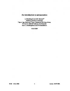
Function metaMDS is a bit special case. The actual ordination is performed by function vegan function monoMDS (or alternatively using isoMDS of the MASS package). Function metaMDS is a wrapper to perform non-metric multidimensional scaling (nmds) like recommended in community ordination: it uses adequate dissimilarity measures (function vegdist), then it runs nmds several times with random starting configurations, compares results (function procrustes), and stops after finding twice a similar minimum stress solution. Finally it scales and rotates the solution, and adds species scores to the configuration as weighted averages (function wascores): > ord ord Call: metaMDS(comm = dune) global Multidimensional Scaling using monoMDS Data: dune Distance: bray Dimensions: 2 Stress: 0.1183186 Stress type 1, weak ties Two convergent solutions found after 20 tries Scaling: centring, PC rotation, halfchange scaling

3

+

1.5

+

1.0

+

●

●

+

+ +

0.5

NMDS2

+ ● ●

+

●

+

+

●

+

0.0

+

+

●

+

+

+

● ●

●

+

+ +

++ +

●

● ●

−0.5

●

+

+ +

●

●

●

+ ●

●

+●

+ +

−1.0

+

−1.0

−0.5

0.0

0.5

1.0

1.5

NMDS1

Figure 1: plot.

Default ordination

Species: expanded scores based on ‘dune’

2

Ordination graphics

Ordination is nothing but a way of drawing graphs, and it is best to inspect ordinations only graphically (which also implies that they should not be taken too seriously). All ordination results of vegan can be displayed with a plot command (Fig. 1): > plot(ord)

Default plot command uses either black circles for sites and red pluses for species, or black and red text for sites and species, resp. The choices depend on the number of items in the plot and ordination method. You can override the default choice by setting type = "p" for points, or type = "t" for text. For a better control of ordination graphics you can first draw an empty plot (type = "n") and then add species and sites separately using points or text functions. In this way you can combine points and text, and you can select colours and character sizes freely (Fig. 2): > plot(ord, type = "n") > points(ord, display = "sites", cex = 0.8, pch=21, col="red", bg="yellow") > text(ord, display = "spec", cex=0.7, col="blue")

All vegan ordination methods have a specific plot function. In addition, vegan has an alternative plotting function ordiplot that also knows many nonvegan ordination methods, such as prcomp, cmdscale and isoMDS. All vegan plot functions return invisibly an ordiplot object, so that you can use ordiplot support functions with the results (points, text, identify). Function ordirgl (requires rgl package) provides dynamic three-dimensional graphics that can be spun around or zoomed into with your mouse. Function ordiplot3d (requires package scatterplot3d) displays simple three-dimensional scatterplots. 4

Empenigr

1.5

Airaprae

1.0

Hyporadi

●

●

Salirepe

Comapalu Vicilath

0.5

NMDS2

Anthodor ● ●

Callcusp

●

Planlanc

Scorautu

0.0

Trifprat Achimill

Eleopalu Ranuflam

● ●

Trifrepe

●

Juncarti

● Rumeacet

Sagiproc●

Bellpere Lolipere Poaprat Bromhord

−0.5

●

●

●

Bracruta

●

Agrostol ● ●

Poatriv

●

●

● Alopgeni Juncbufo ●

Elymrepe Cirsarve

−1.0

Chenalbu

−1.0

−0.5

0.0

0.5

1.0

1.5

NMDS1

2.1

Figure 2: A more colourful ordination plot where sites are points, and species are text.

Cluttered plots

Ordination plots are often congested: there is a large number of sites and species, and it may be impossible to display all clearly. In particular, two or more species may have identical scores and are plotted over each other. Vegan does not have (yet?) automatic tools for clean plotting in these cases, but here some methods you can try: • Zoom into graph setting axis limits xlim and ylim. You must typically set both, because vegan will maintain equal aspect ratio of axes. • Use points and add labell only some points with identify command. • Use select argument in ordination text and points functions to only show the specified items. • Use ordilabel function that uses opaque background to the text: some text labels will be covered, but the uppermost are readable. • Use automatic orditorp function that uses text only if this can be done without overwriting previous labels, but points in other cases. • Use automatic ordipointlabel function that uses both points and text labels, and tries to optimize the location of the text to avoid overwriting. • Use interactive orditkplot function that draws both points and labels for ordination scores, and allows you to drag labels to better positions. You can export the results of the edited graph to encapsulated postscript, pdf, png or jpeg files, or copy directly to encapsulated postscript, or return the edited positions to R for further processing.

2.2

Adding items to ordination plots

Vegan has a group of functions for adding information about classification or grouping of points onto ordination diagrams. Function ordihull adds convex

5

NM

●

0.5

1.0

●

●

●

●

●

●

0.0

● BF ● ●

HF

●

−0.5

NMDS2

●

●

● ●

● ●

●SF ●

●

−0.5

0.0

0.5

1.0

NMDS1

Figure 3: Convex hull, ellipsoid hull, standard error ellipse and a spider web diagram for Management levels in ordination.

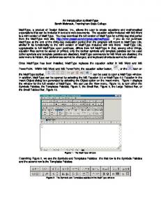
hulls, ordiellipse adds ellipses enclosing all points in the group (ellipsoid hulls) or ellipses of standard deviation, standard error or confidence areas, and ordispider combines items to their centroid (Fig. 3): > data(dune.env) > attach(dune.env) > > > > > >

plot(ord, disp="sites", type="n") ordihull(ord, Management, col=1:4, lwd=3) ordiellipse(ord, Management, col=1:4, kind = "ehull", lwd=3) ordiellipse(ord, Management, col=1:4, draw="polygon") ordispider(ord, Management, col=1:4, label = TRUE) points(ord, disp="sites", pch=21, col="red", bg="yellow", cex=1.3)

In addition, you can overlay a cluster dendrogram from hclust using ordicluster or a minimum spanning tree from spantree with its lines function. Segmented arrows can be added with ordiarrows, lines with ordisegments and regular grids with ordigrid.

3

Fitting environmental variables

Vegan provides two functions for fitting environmental variables onto ordination: • envfit fits vectors of continuous variables and centroids of levels of class variables (defined as factor in R). The arrow shows the direction of the (increasing) gradient, and the length of the arrow is proportional to the correlation between the variable and the ordination. • ordisurf (which requires package mgcv) fits smooth surfaces for continuous variables onto ordination using thinplate splines with cross-validatory selection of smoothness. Function envfit can be called with a formula interface, and it optionally can assess the “significance” of the variables using permutation tests: 6

> ord.fit ord.fit ***VECTORS NMDS1 NMDS2 r2 Pr(>r) A1 0.96474 0.26321 0.3649 0.02 * --Signif. codes: 0 ‘***’ 0.001 ‘**’ 0.01 ‘*’ 0.05 ‘.’ 0.1 ‘ ’ 1 Permutation: free Number of permutations: 999 ***FACTORS: Centroids: NMDS1 NMDS2 ManagementBF -0.4534 -0.0102 ManagementHF -0.2636 -0.1282 ManagementNM 0.2958 0.5790 ManagementSF 0.1506 -0.4670 Goodness of fit: r2 Pr(>r) Management 0.4134 0.006 ** --Signif. codes: 0 ‘***’ 0.001 ‘**’ 0.01 ‘*’ 0.05 ‘.’ 0.1 ‘ ’ 1 Permutation: free Number of permutations: 999

The result can be drawn directly or added to an ordination diagram (Fig. 4): > plot(ord, dis="site") > plot(ord.fit)

Function ordisurf directly adds a fitted surface onto ordination, but it returns the result of the fitted thinplate spline gam (Fig. 4): > ordisurf(ord, A1, add=TRUE) Family: gaussian Link function: identity Formula: y ~ s(x1, x2, k = 10, bs = "tp", fx = FALSE) Estimated degrees of freedom: 1.59 total = 2.59 REML score: 41.58727

4

Constrained ordination

Vegan has three methods of constrained ordination: constrained or “canonical” correspondence analysis (function cca), redundancy analysis (function rda) and distance-based redundancy analysis (function capscale). All these functions 7

1.0

●

●

4.5

0.5

ManagementNM ● ●

A1 ●

●

6.5

0.0

●

3.5

NMDS2

●

●

ManagementBF ●

●

ManagementHF

●

●

●

6

●

5.5

●

−0.5

● ManagementSF ●

5

●

4

●

−0.5

0.0

0.5

1.0

NMDS1

Figure 4: Fitted vector and smooth surface for the thickness of A1 horizon (A1, in cm), and centroids of Management levels.

can have a conditioning term that is “partialled out”. I only demonstrate cca, but all functions accept similar commands and can be used in the same way. The preferred way is to use formula interface, where the left hand side gives the community data frame and the right hand side lists the constraining variables: > ord ord Call: cca(formula = dune ~ A1 + Management, data = dune.env) Inertia Proportion Rank Total 2.1153 1.0000 Constrained 0.7798 0.3686 4 Unconstrained 1.3355 0.6314 15 Inertia is mean squared contingency coefficient Eigenvalues for constrained axes: CCA1 CCA2 CCA3 CCA4 0.3187 0.2372 0.1322 0.0917 Eigenvalues for unconstrained axes: CA1 CA2 CA3 CA4 CA5 CA6 CA7 CA8 CA9 CA10 0.3620 0.2029 0.1527 0.1345 0.1110 0.0800 0.0767 0.0553 0.0444 0.0415 CA11 CA12 CA13 CA14 CA15 0.0317 0.0178 0.0116 0.0087 0.0047

The results can be plotted with (Fig. 5): > plot(ord)

There are three groups of items: sites, species and centroids (and biplot arrows) of environmental variables. All these can be added individually to an empty plot, and all previously explained tricks of controlling graphics still apply. It is not recommended to perform constrained ordination with all environmental variables you happen to have: adding the number of constraints means slacker constraint, and you finally end up with solution similar to unconstrained 8

17

2

19

18

10

11

7 6 5

1

0

2 Achimill Anthodor Bromhord Planlanc Lolipere Poaprat ScorautuManagementHF Trifprat Bellpere Trifrepe ManagementNM Rumeacet Elymrepe Bracruta Poatriv Juncarti Sagiproc Juncbufo4 3 9 Ranuflam Callcusp Alopgeni Cirsarve Agrostol Eleopalu ManagementSF 8 20

−1

CCA2

1

ManagementBF Vicilath

EmpenigrHyporadi Airaprae Salirepe

12 Chenalbu 13

−2

Comapalu

A1 14 15 16

−3

−2

−1

0

1

2

CCA1

Figure 5: Default plot from constrained correspondence analysis.

ordination. In that case it is better to use unconstrained ordination with environmental fitting. However, if you really want to do so, it is possible with the following shortcut in formula: > cca(dune ~ ., data=dune.env) Call: cca(formula = dune ~ A1 + Moisture + Management + Use + Manure, data = dune.env) Inertia Proportion Rank Total 2.1153 1.0000 Constrained 1.5032 0.7106 12 Unconstrained 0.6121 0.2894 7 Inertia is mean squared contingency coefficient Some constraints were aliased because they were collinear (redundant) Eigenvalues for constrained axes: CCA1 CCA2 CCA3 CCA4 CCA5 CCA6 CCA7 CCA8 CCA9 CCA10 0.4671 0.3410 0.1761 0.1532 0.0953 0.0703 0.0589 0.0499 0.0318 0.0260 CCA11 CCA12 0.0228 0.0108 Eigenvalues for unconstrained axes: CA1 CA2 CA3 CA4 CA5 CA6 CA7 0.27237 0.10876 0.08975 0.06305 0.03489 0.02529 0.01798

4.1

Significance tests

vegan provides permutation tests for the significance of constraints. The test mimics standard analysis of variance function (anova), and the default test analyses all constraints simultaneously: > anova(ord) Permutation test for cca under reduced model Permutation: free Number of permutations: 999

9

Model: cca(formula = dune ~ A1 + Management, data = dune.env) Df ChiSquare F Pr(>F) Model 4 0.77978 2.1896 0.001 *** Residual 15 1.33549 --Signif. codes: 0 ‘***’ 0.001 ‘**’ 0.01 ‘*’ 0.05 ‘.’ 0.1 ‘ ’ 1

The function actually used was anova.cca, but you do not need to give its name in full, because R automatically chooses the correct anova variant for the result of constrained ordination. It is also possible to analyse terms separately: > anova(ord, by="term", permutations=199) Permutation test for cca under reduced model Terms added sequentially (first to last) Permutation: free Number of permutations: 199 Model: cca(formula = dune ~ A1 + Management, data = dune.env) Df ChiSquare F Pr(>F) A1 1 0.22476 2.5245 0.010 ** Management 3 0.55502 2.0780 0.005 ** Residual 15 1.33549 --Signif. codes: 0 ‘***’ 0.001 ‘**’ 0.01 ‘*’ 0.05 ‘.’ 0.1 ‘ ’ 1

This test is sequential: the terms are analysed in the order they happen to be in the model. You can also analyse significances of marginal effects (“Type III effects”): > anova(ord, by="mar", permutations=199) Permutation test for cca under reduced model Marginal effects of terms Permutation: free Number of permutations: 199 Model: cca(formula = dune ~ A1 + Management, data = dune.env) Df ChiSquare F Pr(>F) A1 1 0.17594 1.9761 0.050 * Management 3 0.55502 2.0780 0.005 ** Residual 15 1.33549 --Signif. codes: 0 ‘***’ 0.001 ‘**’ 0.01 ‘*’ 0.05 ‘.’ 0.1 ‘ ’ 1

Moreover, it is possible to analyse significance of each axis: > anova(ord, by="axis", permutations=499) Permutation test for cca under reduced model Forward tests for axes Permutation: free Number of permutations: 499 Model: cca(formula = dune ~ A1 + Management, data = dune.env) Df ChiSquare F Pr(>F)

10

CCA1 1 0.31875 3.5801 CCA2 1 0.23718 2.6640 CCA3 1 0.13217 1.4845 CCA4 1 0.09168 1.0297 Residual 15 1.33549 --Signif. codes: 0 ‘***’ 0.001

4.2

0.014 * 0.054 . 0.316 0.412

‘**’ 0.01 ‘*’ 0.05 ‘.’ 0.1 ‘ ’ 1

Conditioned or partial ordination

All constrained ordination methods can have terms that are partialled out from the analysis before constraints: > ord ord Call: cca(formula = dune ~ A1 + Management + Condition(Moisture), data = dune.env) Inertia Proportion Rank Total 2.1153 1.0000 Conditional 0.6283 0.2970 3 Constrained 0.5109 0.2415 4 Unconstrained 0.9761 0.4615 12 Inertia is mean squared contingency coefficient Eigenvalues for constrained axes: CCA1 CCA2 CCA3 CCA4 0.24932 0.12090 0.08160 0.05904 Eigenvalues for unconstrained axes: CA1 CA2 CA3 CA4 CA5 CA6 CA7 CA8 CA9 0.30637 0.13191 0.11516 0.10947 0.07724 0.07575 0.04871 0.03758 0.03106 CA10 CA11 CA12 0.02102 0.01254 0.00928

This partials out the effect of Moisture before analysing the effects of A1 and Management. This also influences the significances of the terms: > anova(ord, by="term", permutations=499) Permutation test for cca under reduced model Terms added sequentially (first to last) Permutation: free Number of permutations: 499 Model: cca(formula = dune ~ A1 + Management + Condition(Moisture), data = dune.env) Df ChiSquare F Pr(>F) A1 1 0.11543 1.4190 0.114 Management 3 0.39543 1.6205 0.016 * Residual 12 0.97610 --Signif. codes: 0 ‘***’ 0.001 ‘**’ 0.01 ‘*’ 0.05 ‘.’ 0.1 ‘ ’ 1

If we had a designed experiment, we may wish to restrict the permutations so that the observations only are permuted within levels of Moisture. Restricted

11

permutation is based on the powerful permute package. Function how() can be used to define permutation schemes. In the following, we set the levels with plots argument: > how anova(ord, by="term", permutations = how) Permutation test for cca under reduced model Terms added sequentially (first to last) Plots: dune.env$Moisture, plot permutation: none Permutation: free Number of permutations: 499 Model: cca(formula = dune ~ A1 + Management + Condition(Moisture), data = dune.env) Df ChiSquare F Pr(>F) A1 1 0.11543 1.4190 0.272 Management 3 0.39543 1.6205 0.004 ** Residual 12 0.97610 --Signif. codes: 0 ‘***’ 0.001 ‘**’ 0.01 ‘*’ 0.05 ‘.’ 0.1 ‘ ’ 1

12