VEGETATION MTF in-flight measurement using HRVIR - OSA Publishing

Edge method for on-orbit defocus assessment Françoise Viallefont-Robinet ONERA DOTA Toulouse, 2, av. E. Belin 31055 Toulouse, France [email protected]

Abstract: In the earth observation domain, two classes of sensors may be distinguished: a class for which sensor performances are driven by radiometric accuracy of the images and a class for which sensor performances are driven by spatial resolution. In this latter case, as spatial resolution depends on the triplet constituted by the Ground Sampling Distance (GSD), Modulation Transfer Function (MTF), and Signal to Noise Ratio (SNR), refocusing, acting as an MTF improvement, is very important. Refocusing is not difficult by itself as far as the on-board mechanism is reliable. The difficulty is on the defocus assessment side. Some methods such as those used for the SPOT family rely on the ability of the satellite to image the same landscape with two focusing positions. This can be done with a bi-sensor configuration, with adequate focal plane, or with the satellite agility. A new generation of refocusing mechanism will be taken aboard Pleiades. As the speed of this mechanism will be much slower than the speed of the older generation, it won’t be possible, despite the agility of the satellite, to image the same landscape with two focusing positions on the same orbit. That’s why methods relying on MTF measurement with edge method have been studied. This paper describes the methods and the work done to assess the defocus measurement accuracy in the Pleiades context. ©2010 Optical Society of America OCIS codes: (110.3000) Image quality assessment; (110.4100) Modulation transfer function; (280.0280) Remote sensing and sensors.

References and links 1. 2. 3. 4. 5. 6. 7. 8. 9.

M. R. B. Forshaw, A. Haskell, P. F. Miller, D. J. Stanley, and J. R. G. Townshend, “Spatial resolution of remotely sensed imagery - A review paper,” Int. J. Remote Sens. 4(3), 497–520 (1983). D. Léger, F. Viallefont, and D. Hillairet, “In-flight refocusing and MTF assessment of SPOT5 HRG and HRS cameras,” Proc. SPIE 4881, 224–231 (2003). W. H. Steel, “The defocused image of sinusoidal gratings,” Opt. Acta (Lond.) 3, 65–74 (1956). K. Maeda, M. Kojima, and Y. Azuma, “Geometric and radiometric performance evaluation methods for marine observation satellite-1 (MOS-1) verification program (MVP),” Acta Astronaut. 15(6-7), 297–304 (1987). T. Choi, “IKONOS satellite in orbit, modulation transfer function measurement using edge and pulse methods”, MSc Thesis, South Dakota State University (2002). F. Lei and H. J. Tiziani, “A comparison of methods to measure the modulation transfer function of aerial survey lens systems from image structures,” Photogramm. Eng. Remote Sensing 54, 41–46 (1988). H. Hwang, Y.-W. Choi, S. Kwak, M. Kim, and W. Park, “MTF assessment of high resolution satellite images using ISO 12233 slanted-edge method,” Proc. SPIE 7109, 710905 (2008). F. Viallefont-Robinet, and D. Léger, “Improvement of the edge method for on-orbit MTF measurement,” Opt. Express 18(4 Issue 4), 3531–3545 (2010), http://www.opticsinfobase.org/oe/abstract.cfm?uri=oe-18-4-3531. A. Rosak, C. Latry, V. Pascal, and D. Laubier, “From SPOT5 to Pleiades-HR: evolutions of the instrumental specifications,” in Proceedings of the 5th international conference on Space Optics, B. Warmbein, ed. (ESA SP-554, Noordwijk, Netherlands, 2004), 141–148.

1. Introduction Spatial resolution of satellite-borne cameras depends on Modulation Transfer Function (MTF) [1]. This important parameter for image quality has to be checked on orbit in order to be sure that launch vibrations, transition from air to vacuum, or thermal state have not spoiled the

#126735 - $15.00 USD

(C) 2010 OSA

Received 8 Apr 2010; revised 3 Jun 2010; accepted 4 Jun 2010; published 12 Oct 2010

27 September 2010 / Vol. 18, No. 20 / OPTICS EXPRESS 20845

sharpness of the images. A part of the potential degradations results in a defocus of the sensor and thus in an MTF decrease. That’s why, at the beginning of the commissioning phase, a defocus measurement is done, leading, if necessary, to refocusing decision. Some focusing measurement methods such as those used for the SPOT family [2] rely on the ability of the satellite to image the same landscape with two focusing positions. This can be done with a bi-sensor configuration, with adequate focal plane, or with the satellite agility. A new generation of refocusing mechanism will be taken aboard Pleiades. As refocusing speed will be much slower than the speed of the older generation, it won’t be possible, despite the agility of the satellite, to image the same landscape with two focusing positions on the same orbit. In this context, this paper presents two methods for defocus measurement, both relying on MTF measurement with the edge method. After a recall of the relationship between defocus and MTF, adaptations of edge method for defocus assessment are described and assessment of defocus measurement accuracy for Pleiades is presented. 2. MTF and defocus Defocus enlarges Point Spread Function (PSF) and decreases MTF. For a diffraction limited sensor with a circular pupil, and a defocus ∆, Steel [3] indicates that monochromatic transfer function can be well approximated by the product of the sensor transfer function without defocus, H0, multiplied by a defocus transfer function, Hdefoc:

H ( f x , f y , ∆ ) = H 0 ( f x , f y , 0) × H defoc ( f x , f y , ∆)

(1)

with

H defoc

 π∆ 2  2 J1  ( f x + f y2 )1/ 2 1 − λ N ( f x2 + f y2 )1/ 2    ( f x , f y , ∆ ) = π∆N 2 2 1/ 2 ( f x + f y ) 1 − λ N ( f x2 + f y2 )1/ 2  N

(2)

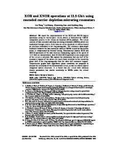
where fx and fy are the spatial frequencies corresponding to the rows (x, across track) and to the columns (y, along track), N the aperture number, and λ the central wavelength. Thanks to this model, if the on-orbit transfer function H0 were known, it would be very simple to deduce the defocus ∆ from an MTF measurement. Unfortunately, launch vibrations, transition from air to vacuum, or thermal state may have modified H0 between ground and space. A first way to deal with this lack of knowledge concerning H0 is to use a parametric H0 model and to find the H0 parameters and the defocus simultaneously by fitting the H model on MTF measurement. The problem is now to measure MTF with an accuracy large enough to assess the defocus. The edge method is a well known and accurate MTF measurement method [4–8]. It could be applied by imaging an artificial edge target such as the Salon-de-Provence one in Fig. 1. Logically, an attempt has been done with this method.

Fig. 1. Salon-de-Provence checkerboard target.

#126735 - $15.00 USD

(C) 2010 OSA



3. Defocus assessment

The first method for defocus assessment consists in fitting an edge computed thanks to the transfer function parametric model with the actual 1D edge [8]. First, an ideal edge is computed. Then, the 1D transfer function is computed in the direction perpendicular to the edge with initial parameter values chosen by the user. A Line Spread Function (LSF) [1] is computed by inverse Fast Fourier Transform of the transfer function. It is then convolved to the ideal edge and the dark and light areas levels are adjusted by linear combination. This produces the computed edge response. The quadratic distance between the actual edge and the computed edge is computed and minimized. This minimization provides adequate values for the parameters of the transfer function model. This method has been applied to simulated Pleiades images [9]. The main conclusion is that the method requires a very large defocus of the edge image in order to be able to distinguish between H0 parameters and defocus. If the defocus is not large enough, the global transfer function measurement is still accurate, but the part of Hdefoc relative to H0 is not well assessed. The large amount of defocus required for the edge image is felt as a weak point of the method. Work has been continued aiming at reducing the required defocus. A second method has been proposed. This second method requires at least three images of the edge corresponding to three known positions of the refocusing mechanism, for instance ps, ps-pk and ps + pk. Noting ∆s the searched defocus corresponding to ps, the defocus values of ps-pk and ps + pk are respectively ∆s-∆k and ∆s + ∆k . ∆k is a known amount of defocus corresponding to the difference of position, pk. pk is chosen large enough in order to have ∆s-∆k < 0 and ∆s + ∆k > 0. For each image, MTF is accurately measured using the edge method described in [8]. In order to lighten the notations, the process will be given for the x direction. The same is done for the y direction. A spatial frequency fd is chosen and MTF = f(fd,0,p) curve, that is to say the MTF curve as a function of refocusing mechanism position p, is drawn for the three positions, ps, ps-pk and ps + pk. For each of these positions, an H value can be computed thanks to (1) by choosing H0 and ∆ values. Thus, model given by (1) can be fitted on the points of the curve MTF = f(fd,0,p). This enables to assess the values of ∆s and H0. Once fitted on the measured MTF, as the maximum of function (2) corresponds to ∆ = 0, the model curve is maximum for the optimal position of the refocusing mechanism. The fit gives the defocus ∆s corresponding to the given position ps as well as the optimal position that is to say the position corresponding to defocus = 0. A first trial has been made using Pleiades simulated images. As the results were very good, a sensitivity study of the method has been performed. 4. PLEIADES results

Hereafter is given a brief summary of the Pleiades [9] features which are of first importance for the defocus assessment: • Aperture number N = 19, • Ratio of diameter of the occultation to the pupil diameter = 0.3, • Perfect square detectors 13 x 13 µm2 wide, • No moving effect (Hmoving = 1). First results

Simulations have been made by P. Kubik in CNES in order to provide images representative of an ideal checkerboard target viewed by a camera having radiometric performances close to Pleiades ones, for three defocus: 0, 400 and 700 µm. The inclination of the edges leads to an oversampling rate of 10.

#126735 - $15.00 USD

(C) 2010 OSA



It is assumed that the defocus is symmetrical: the same simulated image is used for the + 400 or −400 defocus. With this assumption, every combination of three defocus among (−700;-400;0;400;700) can be used. 0, 400 and 700 can be considered as refocusing mechanism positions. The objective is to apply the method and to recover a 0 µm defocus for the 0 µm position, a 400 µm defocus for the 400 µm position and so on. Every combination of three positions among (−700;-400;0;400;700) is used to draw an MTF = f(fd,0,p) curve, even for the delicate cases for which the condition ∆s-∆k < 0 and ∆s + ∆k > 0 is not respected. Model given by (1) is then fitted on the points of the curve MTF = f(fd,0,p). This provides values of ∆s and H0. Choosing for fd the Nyquist frequency, result corresponding to the worst assessment is given in Fig. 2 and Fig. 3. As expected, for this case the condition ∆s-∆k < 0 and ∆s + ∆k > 0 is not respected and thus the model works in extrapolation instead of working in interpolation. Nevertheless, the accuracy is very good (see Fig. 3, MTF for the 0 position should correspond to 0.0 defocus and it is found to be at −32.7 µm of defocus) and below the sensitivity of the focusing mechanism (around 40 µm). Model 0.1

MTF

0.08 0.06 0.04 0.02 0 -800

-600

-400

-200

0

200

400

600

Refocusing mechanism position in µm

Fig. 2. MTF as function of refocusing mechanism position.

0.12

MTF at Nyquist frequency

MTF at Nyquist frequency

0.12

800

0.1

-32.7

0.08

367.3

0.06

667.3

0.04 0.02 0 -200.0

0.0

200.0

400.0

600.0

800.0

Defocus in µm

Fig. 3. Values of defocus of each position.

More representative results

Other simulations have been made starting from actual airborne images of the Salon-deProvence edge target or/and from “Code V” kernels for the PSF. The previous PSF was built thanks to the transfer function model given in section 2. The “Code V” PSF model is of course much representative, mainly for the central obscuration. The previous work has been resumed with simulated images without noise in order to clearly assess the impact of a non ideal target and impact of the difference between the transfer function model and the Pleiades transfer function. Simulated images obtained with Salon-de-Provence edge and previous PSF enables to conclude that the accuracy remains very good: the impacts of edge defaults disappear with replacing the single previous MTF measurement by the mean of the four MTF obtained with the Salon-de-Provence checkerboard. Concerning the case “Code V” PSF and ideal checkerboard, MTF0 = f(fx,0,0), that is to say the MTF curve as a function of frequency without defocus obtained for each edge exhibited a shape unreachable by the H0 model. The impact of the central obscuration was suspected. The decision was taken to choose the frequency fd for which the MTF = f(fd,0, ∆), that is to say the MTF curve as a function of the defocus ∆, was best fitted by the model. Figure 4 shows the variation of the MTF = f(fd,0,∆) curves for different fd values. The value chosen is fd = 0.3fe, noting fe the sampling frequency. At last, simulations with Salon-de-Provence checkerboard, “Code V” PSF, and Pleiades noise were performed and processed. At this stage, the H model will be used twice. First, it will be used to eliminate the noise and thus to reach a very good accuracy for the MTF

#126735 - $15.00 USD

(C) 2010 OSA



measurement for each refocusing mechanism position. Then it will be used as previously described, to assess the defocus ∆s itself. Let’s explain how H model is used twice. In order to reach a good accuracy for the MTF(0.3fe,0,p) measurement, for each p among the three values considered, the H model given by (1) is fitted on each curve MTF = f(fx,0,∆) This first fit gives values for H0 parameters and ∆ but these values are not used because of unreliable unmixing between H0 and Hdefoc as mentioned in paragraph 3. For each p value, H model value for fd = 0.3fe is used to build the MTF = f(0.3fe,0,p) curve. H model given by (1) is then fitted on the points of the curve MTF = f(0.3fe,0,p). This provides accurate values of ∆s and H0. Result corresponding to the worst assessment is given in Fig. 5. Accuracy remains very good (see Fig. 6, MTF for the 0 position should corresponds to 0.0 defocus and it is found to be at −36.5 µm of defocus) and below the sensitivity of the focusing mechanism. 0.2fe case

0.4fe case

0.450

0.250

MTF

model MTFx

0.200

MTFy

0.350 0.300 -1000

-500

0

500

model

MTF

0.400

MTFx MTFy

0.150 0.100 -1000

1000

Defocus (µm)

-500

0

500

1000

Defocus (µm)

0.3fe case

0.5fe case

0.300 0.250 MTF

model MTFx

0.200

MTF

0.160 model 0.110

MTFx

MTFy

0.150 -1000

-500

0

500

MTFy 0.060 -1000

1000

Defocus (µm)

-500

0

500

1000

Defocus (µm)

Fig. 4. Choice of fd frequency. "salon_codeV" case

"salon_codeV" case

0.25

0.25 0.2

-436.5

0.1

-500.0

663.5

0.05

MTF

0 -1000.0

-36.5

0.1

Model

0.05

0.2 0.15

MTF

MTF

0.15

0 0.0

500.0

1000.0

Refocusing mechanism position in µm

Fig. 5. MTF(0.3fe,0,p) as a function of refocusing mechanism position.

-600.0

-400.0

-200.0

0.0

200.0

400.0

600.0

800.0

Defocus in µm

Fig. 6. Values of defocus of each position.

5. Sensitivity study

In order to quantify the impact of the various components of the method, an experiment plan has been carried out. The studied factors were Object (O), Noise (N), Center of the explored range of the focusing mechanism (C), Magnitude of the explored range (M), spatial Frequency

#126735 - $15.00 USD

(C) 2010 OSA



selected fd (F), and Direction of MTF measurement (x or y) (D). The modalities were as follows: For factor O, 2 modalities: ideal target or Salon-de-Provence target, for factor N, 2 modalities: without or with noise, for factor C, 4 modalities: 100, 200, 300, or 400 µm, for factor M, 4 modalities: ± 300, ± 400, ± 500, or ± 600 µm, for factor F, 2 modalities: 0.2 or 0.3fe, for factor D, 2 modalities: x or y. Minimization of the number of experiments was done using a L32(231) Taguchi plan. The table of the variance analysis obtained is given in Table 1, MC being the interaction between factor M and factor C. It shows that every factor except Noise has an actual influence. The predominant factor is the Frequency fd. The experiments also enable to draw the Fig. 7 giving the error on the defocus estimation as a function of factor C for various modalities of factor M. This quantifies the accuracy improvement of the defocus assessment as the Magnitude becomes large enough to ensure case the condition ∆s-∆k < 0 and ∆s + ∆k > 0. All the experiments for which fd = 0.2fe have been replayed using fd = 0.3fe. The curve giving the error on the defocus estimation as a function of factor C for various modalities of factor M is presented in Fig. 8. The accuracy of the defocus assessment as a function of the magnitude of the explored range is given in Table 2. It shows that, without operational constraint, the optimal explored range is M3 (around ± 500 µm): in this case, the accuracy given by the max error is close to the mechanism sensitivity. This table may be used to make a trade-off between refocusing accuracy and operational constraints. Table 1. Variance analysis

Q Liberty degrees S2 Snedecor F

M

C

N

O

F

D

MC

Residue

Total

6541 3

5196 3

2.5 1

4827 1

11438 1

1610 1

6645 9

3781 12

40040 31

2180 6.9

1732 5.5

2.5 0.01

4826 15.3

11438 36.3

1610 5.1

738 2.3

315

1292

3.5

3.5

4.7

4.7

4.7

2.8

2.8

F(0.05) table

Modalities of factor C

C2

C3

Modalities of factor C

C4

C1

120 100

M1 M2

80

M3 M4

60 40 20 0

Fig. 7. Error on defocus measurement as a function of factor C for various modalities of factor M.

#126735 - $15.00 USD

(C) 2010 OSA

Error on defocus assessment (µm)

Error on defocus assessment (µm)

C1

C2

C3

C4

70 60 50 40 30 20 10 0

M1 M2 M3 M4

Fig. 8. Error on defocus measurement with fd = 0.3fe.



Table 2. Error on defocus measurement (µm) Mean error Max error

M1 33 70

M2 32 57

M3 21 32

M4 9 21

6. Conclusion

Two ways of assessing the defocus by edge imaging have been presented and their feasibility has been established in the Pleiades context. For the method relying on three images with various defocus, an assessment of its accuracy and its sensitivity has been carried out still in the Pleiades case. All this work puts forward this method as a reference method for Pleiades. Other methods exist and may be used or tested during the Pleiades commissioning phase, but none of them is as well known considering the accuracy of the defocus measurement. Foreseen work consists in improving the MTF model by taking into account the central obscuration of the pupil. This may lead to a non analytic model. Acknowledgements

We wish to acknowledge the CNES for its funding, and particularly Mr Philippe Kubik, for the Pleiades simulations.

#126735 - $15.00 USD

(C) 2010 OSA

