ABSTRACT. The Tritium Migration Analysis Program, Version 7 (TMAP7) code is an update of TMAP4, an earlier version that was verified and validated in ...
INEEL/EXT-04-01657
Verification and Validation of TMAP7 James Ambrosek Glen R. Longhurst October 2004
Idaho National Engineering and Environmental Laboratory Bechtel BWXT Idaho, LLC
INEEL/EXT-04-01657
Verification and Validation of TMAP7
James Ambrosek Glen R. Longhurst
Published October 2004
Idaho National Engineering and Environmental Laboratory Idaho Falls, Idaho 83415-3860
Prepared for U.S. Department of Energy Office of Science Under DOE-NE-ID Field Office Contract DE-AC07-99ID13727
ii
ABSTRACT The Tritium Migration Analysis Program, Version 7 (TMAP7) code is an update of TMAP4, an earlier version that was verified and validated in support of the International Thermonuclear Experimental Reactor (ITER) program and of the intermediate version TMAP2000. It has undergone several revisions. The current one includes radioactive decay, multiple trap capability, more realistic treatment of heteronuclear molecular formation at surfaces, processes that involve surface-only species, and a number of other improvements. Prior to code utilization, it needed to be verified and validated to ensure that the code is performing as it was intended and that its predictions are consistent with physical reality. To that end, the demonstration and comparison problems cited here show that the code results agree with analytical solutions for select problems where analytical solutions are straightforward or with results from other verified and validated codes, and that actual experimental results can be accurately replicated using reasonable models with this code. These results and their documentation in this report are necessary steps in the qualification of TMAP7 for its intended service.
iii
iv
CONTENTS ABSTRACT ........................................................................................................................... iii 1.0 OVERVIEW ...................................................................................................................... 1 2.0 SPECIALIZED PROBLEMS............................................................................................ 2 2.1 Problem 1a: Diffusion from a Depleting Source (Val-1a)..............................................2 2.2 Problem 1b: Diffusion in a Semi-Infinite Slab with Constant-Source Boundary (Val-1b) ...........................................................................................................................6 2.3 Problem 1c: Diffusion in a Partially Preloaded Semi-Infinite Slab (Val-1c) .................9 2.4 Problem 1d: Permeation Problem with Trapping (Val-1da, Val-1db, Val-1dc)...........12 2.4.1 Effective Diffusivity Trap (Val-1da) .....................................................................13 2.4.2 Strong Trap (Val-1db) ...........................................................................................14 2.4.3 Multiple Trap (Val-1dc) ........................................................................................15 2.5 Problem 1e: Diffusion with Composite Material Layers (Val-1e) ...............................16 2.6 Problem 1f: Heat Sink/Source Problem........................................................................20 2.6.1 Heat conduction with generation (Val-1fa) ...........................................................20 2.6.2 Thermal Diffusion Transient (Val-1fb) .................................................................20 2.6.3 Problem 1fc: Conduction in composite structure with constant surface temperatures (Val-1fc) ....................................................................................................22 2.6.4 Problem 1fd: Convective Heating (Val-1fd) ........................................................25 2.7 Problem 1g: Enclosure Reaction Problems .................................................................27 2.7.1 Simple Forward Reactions (Val-1ga and Val-1gb) ...............................................27 2.7.2 Series Reactions (Val-gc) ......................................................................................30 2.8 Problem 1h: Flow through Multiple Enclosures...........................................................32 2.8.1 Three Enclosure Problem (Val-1ha)......................................................................32 2.8.2 Equilibrating Enclosures (Val-1hb).......................................................................34 2.9 Problem 1i: Species Equilibration on a Reactive Surface ............................................37 2.9.1 Ratedep Conditions................................................................................................37 2.9.2 Surfdep Conditions ................................................................................................39 2.10 Problem 1j: Radioactive Decay ..................................................................................40 2.10.1 Problem 1ja: Radioactive Decay of Mobile Tritium in a Slab (Val-1ja).............40 2.10.2 Problem 1jb: Decay of Tritium in a Distributed Trap (Val-1jb) .........................42 3.0 REPLICATING EXPERIMENTS................................................................................... 44 3.1 Problem 2a: Ion Implantation Experiment (Val-2a)....................................................44
v
3.2 Problem 2b: Diffusion Experiment in Beryllium (Val-2ba, Val-2bb).........................45 3.3 Problem 2c: Test Cell Release Experiment (Val-2c)...................................................47 3.4 Problem 2d: Thermal Desorption Spectroscopy on Tungsten (Val-2d) ......................49 3.5 Problem 2e. Co-permeation of H2 and D2 through Pd..................................................52 4.0 CONCLUSIONS ............................................................................................................. 57 REFERENCES ...................................................................................................................... 59 APPENDIX A SPECIES EQUILIBRATION MODEL.......................................................... 1 Ratedep Conditions.......................................................................................................... A-1 Surfdep Conditions .......................................................................................................... A-3 APPENDIX B PROBLEM INPUT FILE LISTINGS ......................................................... B-1 Problem 1a: Diffusion from a Depleting Source (Val-1a)...............................................B-3 Problem 1b: Diffusion in a Semi-Infinite Slab with Constant-Source Boundary (Val-1b) .......................................................................................................................B-5 Problem 1c Diffusion in a Partially Preloaded Semi-Infinite Slab (Val-1c) ...................B-7 Problem 1da. Effective Diffusivity Trap (Val-1da)..........................................................B-9 Problem 1db. Strong Trap (Val-1db)..............................................................................B-11 Problem 1dc. Multiple Trap (Val-1dc) ...........................................................................B-13 Problem 1e: Diffusion with Composite Material Layers (Val-1e) ................................B-15 Problem 1f: Heat Sink/Source Problem (Val-1fa).........................................................B-17 Problem 1fb. Thermal Diffusion Transient (Val-1fb) ....................................................B-19 Conduction in Composite Structure with Constant Surface Temperatures (Val-1fc) ....B-21 Problem 1fd: Convective Heating (Val-1fd) .................................................................B-23 Problem 1ga: Simple Forward Reactions (Val-1ga)......................................................B-25 Problem 1gb: Simple Forward Reactions (Val-1gb) .....................................................B-27 Problem 1gc: Series Reactions (Val-gc)........................................................................B-29 Problem 1ha: Three Enclosure Problem (Val-1ha) .......................................................B-31 Problem 1hb: Equilibrating Enclosures (Val-1hb) ........................................................B-33 Problem 1ia: Species Equilibration on a Reactive Surface with Equal Starting Pressures (Val-1ia) ....................................................................................................B-35 Problem 1ib: Species Ratedep Equilibration on a Reactive Surface with Unequal Starting Pressures (Val-1ib) ......................................................................................B-37 Problem 1ic: Species Surfdep Equilibration on a Reactive Surface with Equal Starting Pressures (Val-1ic) ....................................................................................................B-39
vi
Problem 1id: Species Surfdep Equilibration on a Reactive Surface with Unequal Starting Pressures (Val-1id) ......................................................................................B-41 Problem 1ja: Radioactive Decay of Mobile Tritium in a Slab (Val-1ja).......................B-43 Problem 1jb: Decay of Tritium in a Distributed Trap (Val-1jb) ...................................B-45 Problem 2a: Ion Implantation Experiment (Val-2a)......................................................B-47 Problem 2b: Diffusion Experiment in Beryllium (Val-2ba, Val-2bb)...........................B-49 Problem 2c: Test Cell Release Experiment (Val-2c).....................................................B-52 Problem 2d: Thermal Desorption Spectroscopy on Tungsten (Val-2d) ........................B-54 Problem 2ea: Permeation of D2 through 0.05-mm Pd at 825 K (Val-2ea) ....................B-57 Problem 2eb: Permeation of D2 through 0.025-mm Pd at 825 K (Val-2eb)..................B-60 Problem 2ec: Permeation of D2 through 0.025-mm Pd at 865 K (Val-2ec) ..................B-63 Problem 2ed: Co-permeation of H2 and D2 through 0.025-mm Pd at 870 K under Law-Dependent Boundary Conditions (Val-2ed) .....................................................B-66 Problem 2ee: Co-permeation of H2 and D2 through 0.025-mm Pd at 870 K under Recombination-Limited Boundary Conditions (Val-2ee).........................................B-69 Problem 2ef: Co-Permeation of H2 and D2 through 0.03-mm Pd at 870 K under Combined Law-Dependent and Recombination-Limited Boundary Conditions (Val-2ef) ....................................................................................................................B-73 FIGURES Figure 1. Fractional release of tritium from an enclosure through SiC in depleting source demonstration problem (Val-1a). ....................................................................................5 Figure 2. Atom flux through outside face of membrane for depleting source problem (Val-1a). ..........................................................................................................................5 Figure 3. Concentration profile in a semi-infinite slab of SiC after 25 s from problem Val1b. ....................................................................................................................................8 Figure 4. Effective-diffusivity, single trap (Val-1da). ...................................................................14 Figure 5. Permeation for strong-trapping regime (Val-1db)..........................................................15 Figure 6. Permeation curve for slab with multiple traps (Val-1dc). ..............................................16 Figure 7. Concentration history 15.75 Pm into the SiC layer of a PyC/SiC composite structure (Val-1e). .........................................................................................................18 Figure 8. Transient temperature distribution for various times in a slab (Val-1fb).......................22 Figure 9. Convective heating at depth 5 cm in a semi-infinite slab (Val-1fd)...............................26 Figure 10. Production of [AB] from [A] and [B] under assumptions of equal and unequal initial reactant concentrations (Val-1ga/Val-1gb).........................................................28 Figure 11. Partial pressures of species in series reaction (Val-1gc). .............................................31 vii
Figure 12. Pressure history of sequentially coupled enclosures (Val-1ha)....................................34 Figure 13. Partial pressure equilibration due to recirculating flow between two enclosures (Val-1hb). ......................................................................................................................36 Figure 14 Species equilibration under ratedep boundary conditions for equal starting pressures of H2 and D2 (Val-1ia)...................................................................................38 Figure 15. Species equilibration under ratedep boundary conditions for unequal starting pressures of H2 and D2 (Val-1ib)...................................................................................38 Figure 16. Species equilibrium under surfdep diffusion boundary conditions for equal starting pressures of H2 and D2 (val-1ic).......................................................................39 Figure 17. Species equilibrium under surfdep diffusion boundary conditions for unequal starting pressures of H2 and D2 (val-1id).......................................................................40 Figure 18. Decay of tritium and associated growth of 3He in a diffusion segment (Val1ja).................................................................................................................................42 Figure 19. Concentration profiles of initially trapped tritium that decayed to 3He over 45 years (Val-1jb)...............................................................................................................43 Figure 20. Concentration of trapped tritium and resulting He-3 over the first 20 years of dedcay............................................................................................................................44 Figure 21. Plasma Driven Permeation of PCA (Val-2a)................................................................45 Figure 22. Thermal desorption test of beryllium (Val-2b). ...........................................................47 Figure 23. HTO Concentration in TSTA Exposure Chamber (Val-2c).........................................48 Figure 24. Schematic of system used to model experiments of Hino et al.23 ................................49 Figure 25. Comparison of calculated with experimental results for Hino's experiment with implantation and thermal desorption of tungsten (Val-2d). ..................................51 Figure 26. Permeability data of Kizu et al. for D2 in Pd................................................................53 Figure 27. TMAP7 model of experimental system of Kizu et al...................................................54 Figure 28. Comparison of TMAP7 permeation calculations with permeation data of Kizu et al. (Val-2ea, Val-2eb, Val-2ec) .................................................................................55 Figure 29. Comparison of TMAP7 results using a lawdep boundary condition on each side of the membrane wirh the experiment s of Kizu et al. (Val-2ed). .........................55 Figure 30. Comparison of TMAP7 calculation with simple ratedep boundary conditions with the values measured by Kizu et al. (Val-2ee)........................................................56 Figure 31. Comparison of TMAP7 calculation for lawdep boundary condition upstream and ratedep boundary condition downstream with measurements made by Kizu et al. (Val-2ef) ...............................................................................................................57
viii
TABLES Table 1. Fractional release of tritium from depleting source problem Val-1a................................ 3 Table 2. Concentration history at x = 0.45 m for problem Val-1b, diffusion in a semi-infinite slab. .................................................................................................................................. 7 Table 3. Concentration Profile (atom/m3) at t = 25 sec for diffusion in a semi-infinite slab. ........ 8 Table 4. Flux (atom/m2 sec) into semi-infinite slab from a constant source................................... 9 Table 5. Concentration history at x = 12 meters. .......................................................................... 10 Table 6. Concentration at x = 0.5 meters ...................................................................................... 11 Table 7. Concentration at x = 10 meters ....................................................................................... 12 Table 8. Steady-state concentration profile in composite slab ..................................................... 17 Table 9. Variance for transient solution in composite slab........................................................... 18 Table 10. Heat Conduction with Generation ................................................................................ 21 Table 11. Temperature distribution in composite structure at t = 150 seconds. ........................... 23 Table 12. Temperature distribution in composite structure at x = 0.09 meters ............................ 24 Table 13. Steady-state temperature distribution for composite structure ..................................... 25 Table 14. Heating of Semi-Infinite Slab by Convection............................................................... 26 Table 15. Concentration of product for equal and unequal starting concentrations. .................... 28 Table 18. Pressure of Species in a Series Reaction ...................................................................... 31 Table 17. Concentration profiles of enclosures 2 and 3 with convective flow............................. 33 Table 19. Concentration of tritium in recirculating convective flow between two enclosures. ... 36 Table 20. Decay of mobile tritium to 3He (Val-1j). ..................................................................... 41
ix
1.0 OVERVIEW The TMAP Code was written at the Idaho National Engineering and Environmental Laboratory by Brad Merrill and James Jones in the late 1980s as a tool for safety analysis of systems involving tritium. 1Since then it has been upgraded to TMAP4 and has been used in numerous applications including experiments supporting fusion safety, predictions for advanced systems such as the International Thermonuclear Experimental Reactor (ITER), and estimates involving tritium production technologies. The code’s further upgrade to TMAP20002 and now to TMAP7 was accomplished in response to several needs. TMAP and TMAP4 had the capacity to deal with only a single trap for diffusing gaseous species in solid structures. TMAP7 includes up to three separate traps and up to 10 diffusing species. The difficulty dealing with heteronuclear molecule formation such as HD under solution-law dependent diffusion boundary conditions, such as Sieverts' law, has been corrected. TMAP7 automatically generates heteronuclear molecular partial pressures and surface flows when solubilities and partial pressures of the homonuclear molecular species are provided. A further sophistication is the addition of non-diffusing surface species. Atoms such as oxygen or nitrogen or complexes such as hydroxyl radicals on metal surfaces are sometimes important in molecule formation with diffusing hydrogen isotopes but do not themselves diffuse appreciably in the material. TMAP7 will accommodate up to 30 such surface species, allowing the user to specify relationships between those surface concentrations and partial pressures of gaseous species above the surfaces or to form them dynamically by combining diffusion species or other surface species. Additionally, TMAP7 allows the user to include a surface binding energy and an adsorption barrier energy and includes asymmetrical diffusion between the surface sites and regular diffusion sites in the bulk. All of the previously existing features for heat transfer, flows between enclosures, and chemical reactions within the enclosures have been retained, but the allowed problem size and complexity have been increased to take advantage of the greater memory and speed available on modern computers. One feature unique to TMAP7 is the addition of radioactive decay for both trapped and mobile species. Another is the ability to initialize distributed parameters such as initial mobile atom, trapped atom, or trap concentrations using selected mathematical functions. Also, time-dependent temperatures and pressures can be specified in boundary enclosures and for surface concentrations of diffusion species. The verification and validation process normally involves two steps. In the verification process, a careful examination of the code ensured that the coding faithfully reproduces the mathematical model and that the code is well written and efficient. That process was pursued extensively with TMAP4. Independent verification has not been done independently of code development for TMAP7. The basic architecture of the code remains the same, although a number of changes were required to work with the GNU FORTRAN 77, selected for distribution with the code. There are also new components and a few new subroutines. These have been carefully evaluated for coding accuracy, but the demonstration of their success is in the high fidelity the code provides to the sample problems. Those sample problems constitute the validation of the code and provide the basis for what is presented here. There are two main sections to this report. The first exercises TMAP7 in each of its major capability areas using specialized problems, showing that the results computed by TMAP7 are in good agreement with “known” results. This demonstrates that the code’s functional tools are
1
performing properly. The second part of the report provides a comparison of TMAP7 results with experimental results to show the general utility of the code in modeling reality. 2.0 SPECIALIZED PROBLEMS Computational capabilities of TMAP7 lie in six major areas: diffusion and trapping within structures and surface processes, heat transfer, chemical reactions in enclosures, bulk fluid flows, chemical equilibrium and radioactive decay. The demonstration problems that follow are grouped into those areas. Problems 1a-1e exercise TMAP7’s mass transfer capabilities Problems 1f (a-d) demonstrate TMAP7's heat transfer functions Problems 1g (a-c) model enclosure reactions Problems 1h (a-b) deal with enclosure flow Problem 1i (a-d) verify chemical reactions in enclosures and on surfaces are correct Problem 1j (a-b) demonstrate radioactive decay. The descriptions of these problems include a statement of the problem, a description of the modeling used in setting up the problem for TMAP7, and a comparison of the TMAP7 results with “known” solutions from literature or other sources. Appendix A is the derivation for the surface equilibrium model used in problem 1i (b). Appendix B contains the input code listings for each of the problems cited in the report. The file names assigned to the various problems appear in parentheses in the headings for the problem descriptions. Input files carry the .inp extension, output or codeout files have .out extensions, and plot data files (pltdata) terminate with the .plt extension. Theoretical results were calculated using Microsoft Excel™, and TMAP7 calculations were obtained in two working environments. One used Windows XP™ on a Dell Optiplex GX 260. The other was Windows ME™ running on a Dell Dimension XPS R450 and on a Dell Latitude 600 laptop computer. 2.1 Problem 1a: Diffusion from a Depleting Source (Val-1a) This diffusion problem models an enclosure that is pre-charged with a fixed quantity of tritium. At time t > 0, the tritium is allowed to diffuse through a finite slab of SiC, initially at zero concentration. The surface of the slab in contact with the source is assumed to be in equilibrium with the source enclosure. The boundary condition at the exit side of the slab is kept constant at zero concentration for all time. The concentration of the enclosure is then calculated for different times and reported as a fractional release. There are no trapping effects active in the slab. Carslaw and Jaeger3 give the analytical solution for an analogous heat transfer problem from which the solute concentration profile in the membrane is C �x, t
f
2 SP0 L ¦ n 1
�
exp � D n2 Dt sin( D n x ) l D n2 � L2 � L sin �D n l
>�
@
2
(1)
where Dn
L
(2)
tan �D n l
STAk V
L
(3)
Here A = cross-sectional area of the slab (2.16 x 10⁻⁶ m2) D = diffusivity of tritium (SiC assumed: 2.6237E-11 m2/s at 2373 K) k = Boltzmann’s constant (1.38065 x 10⁻²³ J/K) l = thickness of the slab (3.30 x 10⁻⁵ m) S = solubility of tritium (SiC assumed: 3.053 x 1029 kg m2/s2) T = temperature (2373 K) V = volume of the enclosure (5.20 x 10⁻¹¹ m3) We apply Henry's law to the concentration at x = l to find the gas pressure in the enclosure P �t
C �l , t S
f
n
�
exp � D n2 Dt 2 2 �L 1 l Dn � L
2 P0 L ¦
�
(4)
and finally the release fraction FR
P �t P0
f
n
�
exp � D n2 Dt 2 2 �L 1 l Dn � L
2 L¦
�
(5)
Some of the values obtained from Equation (5) and from TMAP7 are compared in Table 1. Ten terms were included in the sum of Equation (5) so that even at t = 1 s, the last term was less than 10-10 of the sum. The variance between the analytical solution and the computed solution from TMAP7 is defined by Equation (6). Variance
TMAP7 � Analytical Analytical
(6)
Table 1. Fractional release of tritium from depleting source problem Val-1a. Time 0
TMAP7 0
Theory 0
Variance 0
1
0.166589
0.201078
-0.171524
2
0.242353
0.265929
-0.088655
3
0.291929
0.310049
-0.058444
4
0.329235
0.343941
-0.042757
5
0.359272
0.371571
-0.033099
3
Time 6
TMAP7 0.384472
Theory 0.394945
Variance -0.026516
7
0.406246
0.415252
-0.021687
8
0.425494
0.433273
-0.017954
9
0.442803
0.449553
-0.015015
10
0.458606
0.464482
-0.012651
11
0.473206
0.478348
-0.010751
12
0.486829
0.491366
-0.009233
13
0.499665
0.503693
-0.007997
14
0.511834
0.51545
-0.007015
15
0.523442
0.526726
-0.006234
16
0.534565
0.537588
-0.005623
17
0.545273
0.548089
-0.005139
18
0.555615
0.558269
-0.004754
19
0.565623
0.568157
-0.004459
20
0.575329
0.577778
-0.004238
21
0.584764
0.58715
-0.004063
22
0.593948
0.596289
-0.003926
23
0.602891
0.605206
-0.003825
24
0.611609
0.613913
-0.003753
25
0.620118
0.622417
-0.003693
The variance decreases almost monotonically for t > 25 s. Figure 1 shows the comparison for the first 140 s. A further comparison may be made by noting that the surface flux at x = 0 is J
D
wC �x , t wx x
f
0
2 SP0 LD ¦
n 1
�
exp � D n2 Dt D n l D n2 � L2 � L sin �D n l
>�
@
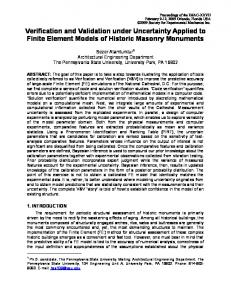
A comparison of results for flux through the free surface is shown in Figure 2.
4
(7)
100.0% 90.0%
Release fraction
80.0% 70.0% 60.0% 50.0% 40.0%
TMAP7
30.0%
Theory
20.0% 10.0% 0.0%
0
20
40
60
80
100
120
140
160
Time (s)
Figure 1. Fractional release of tritium from an enclosure through SiC in depleting source demonstration problem (Val-1a).
1.E+19
Flux at x = 0 (atom/m2s)
1.E+19
TMAP7
1.E+19
Theory 8.E+18 6.E+18 4.E+18 2.E+18 0.E+00 0
20
40
60
80
100
120
140
160
Time (s)
Figure 2. Atom flux through outside face of membrane for depleting source problem (Val-1a).
5
2.2 Problem 1b: Diffusion in a Semi-Infinite Slab with Constant-Source Boundary (Val-1b) This model is designed to test the basic Fick's-law diffusion. A semi-infinite slab is defined with a constant concentration boundary condition. The initial concentration of the slab is zero for time, t d 0 seconds. At time t > 0, the diffusion is allowed to proceed. The slab is assumed to have no traps. Three comparisons are shown; a transient concentration history at a given location, a spatial concentration profile at a given time, and the variation of flux into the slab surface. These are compared with analytical results. Carslaw and Jaeger4 give the analytical solution to the time-dependent concentration profile as § x · ¸¸ . C � x, t C o erfc¨¨ © 2 Dt ¹
(8)
where C(x,t) = diffusion species concentration at position x and time t Co = concentration of the diffusing species at the free surface (1.0 atoms/m3) D = diffusivity (1.0 m2/s). The solution of Equation (8) was found using Microsoft Excel using the series expansion given in CRC Standard Mathematical Tables and Formulae5. This expansion is erfc �x 1� erf �x
2 §� x 3 1 x 5 1 x 7 1 x 9 ·� 1� � � ...¸�. ¨�x � � 3 2! 5 3! 7 4! 9 ¹� S ©�
(9)
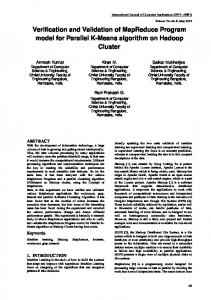
Twenty-five terms were taken in this expansion with the last term contributing less than 1.0 x 10⁻¹¹ at the full depth of the model. Two comparisons were made for this model between the values of Equation (8) and results from TMAP7. The first comparison was made for the concentration at times ranging from t = 0 to 30 s at a distance from the surface of x = 0.45 m. The disagreement between Equation (8) and TMAP7 was less than 0.02% at t = 1 sec. The variance decreased with time, declining quickly to 0.001%. These values are listed in Table 2. The second comparison examined the concentration profile from x = 0.005 to 0.195 m at increments of 0.01 m at time, t = 25 s. The variance between Equation (8) and TMAP7 is small, exceeding 0.1% only at depths greater than 11 m. The comparison of these values can be seen in Table 3 and in Figure 3.
6
Table 2. Concentration history at x = 0.45 m for problem Val-1b, diffusion in a semi-infinite slab. Time 0 1 2 3 4 5 6 7 8 9 10 11 12 13 14 15 16 17 18 19 20 21 22 23 24 25 26 27 28 29 30
TMAP7 0.00000 0.74926 0.82158 0.85402 0.87345 0.88674 0.89656 0.90421 0.91038 0.91549 0.91981 0.92354 0.92678 0.92965 0.93221 0.93450 0.93658 0.93847 0.94020 0.94179 0.94326 0.94463 0.94590 0.94709 0.94820 0.94925 0.95023 0.95116 0.95204 0.95287 0.95367
Theory 0.00000 0.75033 0.82198 0.85424 0.87359 0.88684 0.89664 0.90427 0.91043 0.91553 0.91985 0.92357 0.92681 0.92968 0.93223 0.93452 0.93660 0.93848 0.94021 0.94181 0.94328 0.94464 0.94591 0.94710 0.94821 0.94926 0.95024 0.95117 0.95205 0.95288 0.95367
Variation 0.00000 -0.00143 -0.00049 -0.00026 -0.00016 -0.00011 -0.00009 -0.00007 -0.00005 -0.00004 -0.00004 -0.00003 -0.00004 -0.00003 -0.00002 -0.00002 -0.00002 -0.00002 -0.00002 -0.00002 -0.00002 -0.00001 -0.00001 -0.00001 -0.00001 -0.00001 -0.00001 -0.00001 -0.00001 -0.00001 0.00000
7
Table 3. Concentration Profile (atom/m3) at t = 25 sec for diffusion in a semi-infinite slab.
Concentration (atom/m3)
X (m) 0.00 0.05 0.15 0.25 0.35 0.45 0.55 0.65 0.75 0.85 0.95 1.05 1.15 1.25 1.35 1.45 1.55 1.65 1.75 1.85 1.95
TMAP7 1.00000 0.99436 0.98307 0.97179 0.96052 0.94925 0.93799 0.92675 0.91551 0.90430 0.89311 0.88193 0.87078 0.85966 0.84856 0.83750 0.82646 0.81546 0.80450 0.79357 0.78269
Theory 1.00000 0.99436 0.98308 0.97180 0.96052 0.94926 0.93800 0.92676 0.91553 0.90432 0.89313 0.88195 0.87081 0.85968 0.84859 0.83752 0.82649 0.81549 0.80453 0.79361 0.78272
Variation 0.00000 0.00000 -0.00001 -0.00001 0.00000 -0.00001 -0.00001 -0.00001 -0.00002 -0.00002 -0.00002 -0.00003 -0.00003 -0.00003 -0.00003 -0.00003 -0.00004 -0.00004 -0.00004 -0.00005 -0.00004
1.2 1.0 0.8
TMAP7 Theory
0.6 0.4 0.2 0.0 0
5
10
15
20
Depth (m) Figure 3. Concentration profile in a semi-infinite slab of SiC after 25 s from problem Val-1b.
8
The third, and final, comparison for this problem was the comparison of the diffusive flux into the slab. The flux into or out of a slab is proportional to the concentration gradient in the x direction at the slab surface. The solution6 is given by J
Co
§ x · D exp¨¨ ¸¸ tS © 2 Dt ¹
(10)
The values of Equation (10) were found using Microsoft Excel. They were compared to the values obtained from TMAP7 and can be seen in Table 4. The variance is never greater than 0.44%. Table 4. Flux (atom/m2 sec) into semi-infinite slab from a constant source Time (s) TMAP7 0 0.00000 1 0.56668 2 0.39982 3 0.32621 4 0.28240 5 0.25253 6 0.23050 7 0.21338 8 0.19958 9 0.18815 10 0.17849 11 0.17018 12 0.16293 13 0.15653 14 0.15083 15 0.14572 16 0.14109 17 0.13687 18 0.13301 19 0.12946 20 0.12618 21 0.12314 22 0.12031 23 0.11766 24 0.11519 25 0.11286 26 0.11067 27 0.10860 28 0.10664 29 0.10478 30 0.10302
Theory Variance 0.00000 0.00000 0.56419 0.00441 0.39894 0.00220 0.32574 0.00146 0.28209 0.00108 0.25231 0.00086 0.23033 0.00074 0.21324 0.00064 0.19947 0.00055 0.18806 0.00046 0.17841 0.00043 0.17011 0.00041 0.16287 0.00038 0.15648 0.00033 0.15079 0.00029 0.14567 0.00032 0.14105 0.00030 0.13684 0.00025 0.13298 0.00022 0.12943 0.00020 0.12616 0.00019 0.12312 0.00019 0.12029 0.00020 0.11764 0.00016 0.11516 0.00022 0.11284 0.00020 0.11065 0.00021 0.10858 0.00020 0.10662 0.00017 0.10477 0.00012 0.10301 0.00013
2.3 Problem 1c: Diffusion in a Partially Preloaded Semi-Infinite Slab (Val-1c) This problem models a semi-infinite slab with the first 10 meters preloaded to a uniform concentration. The concentration at the free surface is set to zero for time, t t 0 sec, when the 9
pre-loaded inventory is allowed to diffuse out the surface and through the slab. No traps are assumed to be present. Comparisons are made between TMAP7 and analytical values for concentration histories at two locations: one in the initially unloaded region of the slab, at x = 12 m, and one near the surface, x = 0.25 m. A third is made at the end of the preloaded region. By analogy with Carslaw and Jaeger7 the concentration as a function of space and time is C
Co ª § x · § x�h · § h � x ·º ¸¸ � erf ¨¨ ¸¸ � erf ¨¨ ¸¸» «2erf ¨¨ 2 ¬ © 2 Dt ¹ © 2 Dt ¹ © 2 Dt ¹¼
where h = thickness of pre-loaded region in the slab (10 m) Co = concentration of pre-loaded section (1.0 atoms/m3) D = diffusion coefficient (1.0 m2/sec) Results for the concentration history at x = 12 m can be seen in Table 5. Except for very short times when the theoretical solution has difficulty with evaluation, the variance for this problem never exceededs 0.7%. Table 5. Concentration history at x = 12 meters. Time 0 5 10 15 20 25 30 35 40 45 50 55 60 65 70 75 80 85 90 95 100
TMAP7 0.00000 0.26268 0.31901 0.32806 0.31762 0.29938 0.27872 0.25813 0.23868 0.22078 0.20452 0.18984 0.17661 0.16470 0.15397 0.14426 0.13548 0.12752 0.12026 0.11365 0.10760
Theory Variance 1 0.00000 0.00000 0.263545 -0.003281 0.322467 -0.010721 0.329065 -0.003054 0.318136 -0.001638 0.298963 0.001379 0.276791 0.006949 0.257558 0.002203 0.238604 0.000317 0.220764 0.000071 0.204491 0.000142 0.189789 0.000243 0.176548 0.000354 0.164626 0.000450 0.153881 0.000546 0.144178 0.000566 0.135397 0.000614 0.127429 0.000674 0.12018 0.000662 0.113569 0.000672 0.107522 0.000678
The next comparison for this model is at x = 0.5 m, the closest node to the surface. The variance for this problem was less than 1 % for times, t t 15 sec. Again, at short times the theoretical solution is imprecise. These values can be seen in Table 6.
10
(11)
Table 6. Concentration at x = 0.5 meters Time 0 5 10 15 20 25 30 35 40 45 50 55 60 65 70 75 80 85 90 95 100
0.5 m 1.00000 0.12689 0.08250 0.05951 0.04532 0.03590 0.02930 0.02448 0.02084 0.01801 0.01577 0.01395 0.01246 0.01122 0.01016 0.00927 0.00849 0.00782 0.00723 0.00672 0.00626
Theory 1.000000 0.139547 0.081585 0.058933 0.044912 0.035599 0.029074 0.024306 0.020702 0.017904 0.015681 0.01388 0.012399 0.011162 0.010118 0.009227 0.008459 0.007791 0.007207 0.006693 0.006236
Variance 0.00000 -0.09070 0.01123 0.00982 0.00915 0.00845 0.00778 0.00713 0.00660 0.00609 0.00571 0.00532 0.00495 0.00472 0.00444 0.00420 0.00399 0.00379 0.00362 0.00346 0.00331
The last comparison is made at x = h. For this case, Equation (11) reduces to C
Co 2
ª § h · § h � x ·º ¸¸ � erf ¨¨ ¸¸» . «2erf ¨¨ © 2 Dt ¹ © 2 Dt ¹¼ ¬
(12)
The variance between the values obtained from TMAP7 and Equation (12) has the largest values at times, t d 20 sec. For all other times, the variance is less than 0.1 %. The comparison of TMAP7 calculated values with theory may be seen in Table 7.
11
Table 7. Concentration at x = 10 meters Time 0 5 10 15 20 25 30 35 40 45 50
TMAP7 0.50000 0.49780 0.47344 0.43138 0.38646 0.34482 0.30816 0.27647 0.24923 0.22580 0.20559
Theory Variance 1 0.50000 0 0.49838 -0.00117 0.47465 -0.00257 0.43211 -0.0017 0.38615 0.00078 0.34498 -0.00046 0.30821 -0.00017 0.27642 0.000177 0.24912 0.000417 0.22567 0.00059 0.20544 0.000732
2.4 Problem 1d: Permeation Problem with Trapping (Val-1da, Val-1db, Val-1dc) The following three models simulate diffusion through a slab in which traps are operational. The three trapping regimes demonstrated are an effective diffusivity trap, a strong trap, and a set of three traps in the effective diffusivity range with different trap strengths. The diffusion boundary conditions for this set of problems are fixed-concentration or sconc, with one surface kept at a constant non-zero concentration and the other set at zero concentration. Initially, the slab is empty. Validation criteria for these problems will be the comparison of the flux and breakthrough times for each of the models with idealizations. The breakthrough time of the flux may have one of two limiting values, which depend on whether the trapping is in the effective diffusivity or strong-trapping regime. A trapping parameter8 is defined by
]
O2X § E �H · exp¨ d ¸ Do U © kT ¹
(13)
where O = lattice parameter (assume 3.162 x 10⁻⁸ m) Q = Debye frequency (1 x 10¹³ s-1) U = trapping site fraction (0.1) Do = diffusivity pre-exponential (1 m2/sec) Ed = diffusion activation energy (assume 0 eV) H = trap energy k = Boltzmann’s constant T = temperature (1000 K) The determining value for which regime is dominant is the relation of ] to c/U where c is the surface concentration of the mobile species normalized to the lattice density (0.0001 here).
12
2.4.1 Effective Diffusivity Trap (Val-1da) If ] !! c/U, then the effective diffusivity regime applies, and the flux transient is nearly identical to the standard diffusion transient, but with the diffusivity replaced by an effective diffusivity, Deff
D 1� ¦ i
(14)
1
9i
In this limit, the breakthrough time, defined as the intersection of the steepest tangent of the diffusion transient with the time axis, will be
Wb
e
l2 2S 2 Deff
(15)
where l = thickness of slab (1 m) Deff = effective diffusivity of gas (m2/s). The permeation transient is then given by Jp
f § co D ª t m «1 � 2¦ �� 1 exp¨ � m 2 ¨ l «¬ 2W be m 1 ©
·º ¸» ¸» ¹¼
(16)
where Wbe is as defined in Equation (15). The first example is the case where a single trap is in the effective diffusivity limit. The ratio H/k (see Equation (13)) was taken as 100, to give a value of ] = 90.49 c/U. TMAP7's breakthrough time was found numerically by using a three-point differentiation method given by Fogler9 to find the steepest slope. § dC A · ¨ ¸ © dt ¹ ti
1 >C A�i �1 � C A�i �1 @ | m 2't
(17)
Then, the point where the slope was the steepest was used with the slope at that point to find the intersection with the time axis. This was computed to be 0.629 seconds. The analytical breakthrough time (plotted) was calculated to be 0.611 seconds. The variance between theoretical values of the permeation flux and those calculated by TMAP7 using this model is less than 1%, for times greater than 1 second, as shown in Figure 4. The permeation curve where no trapping is present is also shown in Figure 4 to illustrate the retarding of the permeation curve by a trap.
13
4.0E+18
Flux (atom/m2.s)
3.5E+18
TMAP7 Permeation
3.0E+18
Steepest Tangent
2.5E+18 2.0E+18
Effective Diffusivity Limit
1.5E+18
No Trapping
1.0E+18
Breakthrough
5.0E+17 0.0E+00 0
1
2
3
4
Time (s) Figure 4. Effective-diffusivity, single trap (Val-1da). 2.4.2 Strong Trap (Val-1db) In the second model, ] k �l � x On @ Co ® � 2¦ exp � DPyC O2nt 2 2 On a sin klOn � l sin �aOn °¯ lDPyC � aDSiC n 1
>
�
where a = thickness of PyC (33 Pm)
17
@
�
½
°¾ °¿
(21)
l = Thickness of SiC (63 Pm) k
DPyC DSiC
69.7036
and the On are the roots of tan �O a � k tan �k O l 0
(22)
Concentration (atm/m3)
Figure 7 shows the graphical comparison, and Table 9 lists discreet values and variance. The fit would be better with a finer spatial mesh.
3.E+25
2.E+25 TMAP7 Theory
1.E+25
-4.E+09 0
10
20
30
40
50
60
Time (s) Figure 7. Concentration history 15.75 Pm into the SiC layer of a PyC/SiC composite structure (Val-1e). Table 9. Variance for transient solution in composite slab. Time (s) 0
TMAP7 0.0000E+00
Theory 0.0000E+00
Variance 0.00000
1
1.1763E+24
8.9218E+23
0.31846
2
3.3680E+24
3.7714E+24
-0.10697
3
5.6012E+24
6.3731E+24
-0.12112
4
7.5856E+24
8.4393E+24
-0.10116
5
9.2734E+24
1.0086E+25
-0.08061
6
1.0694E+25
1.1427E+25
-0.06416
7
1.1893E+25
1.2542E+25
-0.05172
8
1.2913E+25
1.3485E+25
-0.04242
9
1.3791E+25
1.4296E+25
-0.03535
10
1.4555E+25
1.5003E+25
-0.02987
18
Time (s) 11
TMAP7 1.5225E+25
Theory 1.5626E+25
Variance -0.02566
12
1.5819E+25
1.6180E+25
-0.02230
13
1.6350E+25
1.6677E+25
-0.01959
14
1.6828E+25
1.7125E+25
-0.01736
15
1.7261E+25
1.7533E+25
-0.01551
16
1.7655E+25
1.7905E+25
-0.01399
17
1.8015E+25
1.8247E+25
-0.01272
18
1.8346E+25
1.8562E+25
-0.01164
19
1.8651E+25
1.8853E+25
-0.01072
20
1.8933E+25
1.9123E+25
-0.00993
21
1.9195E+25
1.9374E+25
-0.00922
22
1.9438E+25
1.9607E+25
-0.00863
23
1.9665E+25
1.9825E+25
-0.00808
24
1.9877E+25
2.0029E+25
-0.00758
25
2.0075E+25
2.0219E+25
-0.00714
26
2.0260E+25
2.0398E+25
-0.00676
27
2.0433E+25
2.0565E+25
-0.00644
28
2.0596E+25
2.0722E+25
-0.00610
29
2.0749E+25
2.0870E+25
-0.00580
30
2.0892E+25
2.1009E+25
-0.00555
31
2.1027E+25
2.1139E+25
-0.00530
32
2.1154E+25
2.1261E+25
-0.00505
33
2.1274E+25
2.1377E+25
-0.00481
34
2.1386E+25
2.1485E+25
-0.00462
35
2.1492E+25
2.1587E+25
-0.00441
36
2.1592E+25
2.1683E+25
-0.00421
37
2.1686E+25
2.1774E+25
-0.00403
38
2.1774E+25
2.1859E+25
-0.00389
39
2.1858E+25
2.1939E+25
-0.00370
40
2.1936E+25
2.2015E+25
-0.00358
41
2.2011E+25
2.2086E+25
-0.00340
42
2.2081E+25
2.2153E+25
-0.00325
43
2.2146E+25
2.2216E+25
-0.00316
44
2.2209E+25
2.2276E+25
-0.00300
45
2.2267E+25
2.2332E+25
-0.00290
46
2.2323E+25
2.2385E+25
-0.00276
47
2.2375E+25
2.2434E+25
-0.00265
48
2.2424E+25
2.2481E+25
-0.00255
19
Time (s) 49 50
TMAP7 2.2471E+25
Theory 2.2526E+25
Variance -0.00242
2.2515E+25
2.2567E+25
-0.00231
2.6 Problem 1f: Heat Sink/Source Problem Heat transfer models were set up to validate the heat transfer capabilities of the TMAP7 code. The four problems solved include (a) heat conduction with generation; (b) transient conduction and steady state values in a composite structure, and (c) heating of a semi-infinite slab by convection, and (d) convective heating. 2.6.1 Heat conduction with generation (Val-1fa) To model the first problem, the thermal boundary conditions were set so one surface was adiabatic, while the other was kept at constant temperature. The heat generation in the slab was assumed to be constant throughout. Incropera and DeWitt10 give the analytical solution for the steady state temperature of this model as T
Ts �
QL2 2k
§ x2 · ¨¨1 � 2 ¸¸ © L ¹
(23)
where Q = internal heat generation rate (10,000 W/m3) L = thickness of slab (1.6 m) k = thermal conductivity (10 W/m K) Ts = surface temperature (300 K) A value for thermal mass, the product of material mass density and specific heat, must be added for TMAP7 thermal calculations. In this problem, Ucp = 1 J/m3K was assumed. Initially, 16 spatial segments were assumed. The variance for this problem was less than 0.2% for distances less than 1.35 m, but it increased as the distance from the adiabatic surface was increased. To show that this can be reduced with a decrease in the distance between nodes, an additional calculation was performed with 48 spatial segments. The variance was reduced by a factor of approximately 10. The comparison of Equation (23) with TMAP7 values can be seen in Table 10. 2.6.2 Thermal Diffusion Transient (Val-1fb) The second problem validates the thermal diffusion capability in a slab. The temperature of the left side of the thermal segment was held constant at 400 K while the right side was held at a constant 300 K. The initial temperature in the slab was 300 K. For this example, the thickness, L, was 3.75 m and the heat production rate was Q = 0. Diffusion was ignored by setting the mobile species concentration to zero and using non-flow boundaries. The analytical solution is given by ª x 2 f 1 º T � x, t To � �T1 � To «1 � � ¦ sin �O m x exp � DO2m t » ¬ L L m 0 Om ¼
�
20
(24)
Table 10. Heat Conduction with Generation Position (m) Theory 0.00 1580.00 0.05 1578.75 0.15 1568.75 0.25 1548.75 0.35 1518.75 0.45 1478.75 0.55 1428.75 0.65 1368.75 0.75 1298.75 0.85 1218.75 0.95 1128.75 1.05 1028.75 1.15 918.75 1.25 798.75 1.35 668.75 1.45 528.75 1.55 378.75 1.60 300.00
16 Segs Variance 48 Segs Variance 1580.00 0.00000 1580.00 0.00000 1580.00 0.00079 1578.90 0.00010 1570.00 0.00080 1568.90 0.00010 1550.00 0.00081 1548.90 0.00010 1520.00 0.00082 1518.90 0.00010 1480.00 0.00085 1478.90 0.00010 1430.00 0.00087 1428.90 0.00010 1370.00 0.00091 1368.90 0.00011 1300.00 0.00096 1298.90 0.00012 1220.00 0.00103 1218.90 0.00012 1130.00 0.00111 1128.90 0.00013 1030.00 0.00122 1028.90 0.00015 920.00 0.00136 918.88 0.00014 800.00 0.00156 798.88 0.00016 670.00 0.00187 668.88 0.00019 530.00 0.00236 528.88 0.00025 380.00 0.00330 378.89 0.00037 300.00 0.00000 300.00 0.00000
where
Om
m
S L
(25)
and thermal diffusivity is
D
k
(26)
CpU
For the problem analyzed, D = 1.0 m2/s, To = 300 K, and T1 = 400 K. The values for Equation (24) were found using Microsoft Excel. The last term in the summation taken contributed less than 1 x 10-13 of the theoretical value. The agreement between TMAP7 and Equation (24) is excellent, with the variance less than 1 % for each case tested, and usually much less. The comparison between the values can be seen in Figure 8 for temperature profiles through the slab at 0.1, 0.5, 1.0, and 5.0 seconds.
21
400.00 TMAP7 Theory 0.1 s TMAP7 Theory 0.5 s TMAP7 Theory 1.0 s TMAP7 Theory 5.0 s
390.00
Temperature (K)
380.00 370.00 360.00 350.00 340.00 330.00 320.00 310.00 300.00 0
0.5
1
1.5
2
2.5
3
3.5
4
Depth (m)
Figure 8. Transient temperature distribution for various times in a slab (Val-1fb).
2.6.3 Problem 1fc: Conduction in composite structure with constant surface temperatures (Val-1fc) The third heat transfer problem studied was heat transfer through a composite with constant surface temperatures. The composite was a 40-cm thick layer of Cu followed by a 40-cm layer of Fe. The temperature of both layers was initially 0 K, but at time t = 0, the outside face of the copper was held at 600 K while the outside face of the Fe was maintained at 0 K. This problem was modeled using the heat transfer capability of TMAP7. The computational answers obtained by TMAP7 for both the transient and steady state solutions were compared to values obtained from ABAQUS.11 The ABAQUS code was setup and run by R. G. Ambrosek. ABAQUS is a heat transfer program that has been validated for both transient and steady state solutions. The transient solution was compared at a constant time and constant distance. The constant time comparison between ABAQUS and TMAP7 was made at time, t = 150 sec. The variance in this comparison grows with increasing distance. This may be due to the time interval on both programs being larger than needed, or round-off error from the printed values. These values can be seen in Table 11.
22
Table 11. Temperature distribution in composite structure at t = 150 seconds. Distance (m) ABAQUS 0 600.000 0.01 574.400 0.03 523.600 0.05 473.600 0.07 425.100 0.09 378.400 0.11 334.100 0.13 292.500 0.15 253.900 0.17 218.500 0.19 186.400 0.21 157.700 0.23 132.200 0.25 110.000 0.27 90.790 0.29 74.480 0.31 60.860 0.33 49.690 0.35 40.770
TMAP7 600.000 574.370 523.400 473.310 424.630 377.890 333.500 291.850 253.210 217.780 185.680 156.940 131.530 109.340 90.237 74.026 60.505 49.457 40.669
Variance 0.00000 -0.00005 -0.00038 -0.00061 -0.00111 -0.00135 -0.00180 -0.00222 -0.00272 -0.00330 -0.00386 -0.00482 -0.00507 -0.00600 -0.00609 -0.00610 -0.00583 -0.00469 -0.00248
The values were also compared at x = 0.09 m, at 5 second intervals from time t = 0 to 150 sec. The variance is initially large, but reduces as the time increases. The initially large variance may be due to the same factors of spatial resolution and time step size mentioned earlier. These results can be seen in Table 12. The steady-state solution for this problem was compared to the analytical solution in addition to the ABAQUS answer. To solve for the steady state solution for this problem, the heat flux is given by q ''
TS A � TS B L A LB � kA kB
(27)
where Tsi = Temperature of surface i, left (A) and right (B), Li = Length of segment i ki = thermal conductivity of segment i. For the solution to be at steady state, the flux in and out of any section of the slab must be equal. The temperature at the interface can be found by setting the flux through A equal to the flux through B.
23
Table 12. Temperature distribution in composite structure at x = 0.09 meters Time (s) 0 5 10 15 20 25 30 35 40 45 50 55 60 65 70 75 80 85 90 95 100 105 110 115 120 125 130 135 140 145 150
TS A � TI LA kA
TMAP 7 0 6.78 37.14 75.02 11.23 140.78 166.96 189.48 209.02 226.12 241.23 254.69 266.78 277.70 287.63 296.71 305.05 312.74 319.86 326.49 332.67 338.45 343.87 348.98 353.79 358.33 362.64 366.73 370.61 374.31 377.89
ABAQUS 0 10.11 43.47 81.42 115.90 145.60 171.10 193.10 212.10 228.90 243.70 256.90 268.70 279.50 289.36 298.30 306.40 314.00 321.00 327.60 333.70 339.40 344.80 349.80 354.60 359.10 363.40 367.40 371.30 374.90 378.40
Variance 0.0000 -0.3290 -0.1456 -0.0786 -0.9031 -0.0331 -0.0242 -0.0187 -0.0145 -0.0121 -0.0101 -0.0086 -0.0071 -0.0064 -0.0060 -0.0053 -0.0044 -0.0040 -0.0036 -0.0034 -0.0031 -0.0028 -0.0027 -0.0023 -0.0023 -0.0021 -0.0021 -0.0018 -0.0019 -0.0016 -0.0013
TI � TS B
(28)
LB kB
where TI = temperature of interface, kA = 401 W /m K, kB = 80.2 W /m K, LA = LB = 0.4 meters, TS A = 600 K
TS B = 0 K
24
From Equation (28), the interface temperature is found to be TI = 500 K. The temperature profile for conduction in steady state, with constant physical properties, is linear. The temperature profile of A and B can be found through linear interpolation. The comparison of TMAP7, ABAQUS, and the analytical solution were found to be identical. These values can be seen in Table 13. Table 13. Steady-state temperature distribution for composite structure Distance (m) 0.00 0.01 0.03 0.05 0.07 0.09 0.11 0.13 0.15 0.17 0.19 0.21 0.23 0.25 0.27 0.29 0.31 0.33 0.35
TMAP7 600.0 597.5 592.5 587.5 582.5 577.5 572.5 567.5 562.5 557.5 552.5 547.5 542.5 537.5 532.5 527.5 522.5 517.5 512.5
ABAQUS 600.0 597.5 592.5 587.5 582.5 577.5 572.5 567.5 562.5 557.5 552.5 547.5 542.5 537.5 532.5 527.5 522.5 517.5 512.5
Theory 600.0 597.5 592.5 587.5 582.5 577.5 572.5 567.5 562.5 557.5 552.5 547.5 542.5 537.5 532.5 527.5 522.5 517.5 512.5
2.6.4 Problem 1fd: Convective Heating (Val-1fd) The fourth heat transfer problem modeled was the heating of a semi-infinite slab by convection at the boundary. The slab was initially configured with a constant temperature of 100 K throughout the slab. A convection boundary was then activated at the surface for time, t t 0 sec. Incorpera and DeWitt10 give for the solution °ª § x T � x, t Ti � �Tf � Ti ®«erfc¨ © 2 tD °¯¬
·º ª §¨ hx h 2tD ·¸º ¸» � «exp¨ � 2 ¸» k ¹»¼ ¹¼ «¬ © k
where Ti = initial temperature (100 K) Tf = temperature of enclosure (500 K) h = conduction coefficient (200 W/m2 K) k = thermal conductivity (801 W/m K)
D = thermal diffusivity (1.17 x 10⁻⁴ m2/s )
25
ª § x h tD ·º ½° ¸» ¾ � «erfc¨¨ k ¸¹»¼ °¿ «¬ © 2 tD
(29)
The depth x of 5 cm was used for comparison. Values of the complimentary error function were computed using a series expansion in Microsoft Excel. The last term computed contributed less than 1.0 x 10-120. The variance between Equation (29) and TMAP7 was less than 0.2%, for all times greater than 30 sec, as can be seen in Table 14. A graphical comparison can be seen in Figure 9. Table 14. Heating of Semi-Infinite Slab by Convection Time (s) 0 10 20 30 40 50 60 70 80 90 100 110 120 130 140 150 160 170 180
TMAP 7 100.00 102.14 104.06 105.80 107.39 108.86 110.23 111.51 112.72 113.86 114.94 115.98 116.97 117.92 118.84 119.72 120.58 121.41 122.21
Theory 100.00 100.00 103.64 105.55 107.25 108.79 110.21 111.53 112.76 113.92 115.02 116.06 117.06 118.02 118.95 119.83 120.69 121.52 122.33
Variance 0.00000 0.02140 0.00406 0.00238 0.00129 0.00060 0.00017 -0.00015 -0.00033 -0.00051 -0.00067 -0.00072 -0.00081 -0.00088 -0.00089 -0.00095 -0.00093 -0.00093 -0.00097
Temperature (K)
175 150 Theory TMAP7
125 100 0
200
400
600
800 1000 1200 1400
Time (s) Figure 9. Convective heating at depth 5 cm in a semi-infinite slab (Val-1fd)
26
2.7 Problem 1g: Enclosure Reaction Problems Three problems were solved in TMAP7 to test its capability to handle enclosure reactions. The first model is a simple forward reaction with two reactants forming one product. In the first model, the reactants start in their stoichiometric ratio. The second problem varies from the first in that the concentrations of the reactants vary from their stoichiometric ratio. The third problem examines a series reaction. 2.7.1 Simple Forward Reactions (Val-1ga and Val-1gb) The first and second problems consider the simple chemical reaction A � B o AB .
(30)
The rate at which the concentrations change (rate of reaction) is assumed first order with respect to the concentrations of A and B. The rate coefficient, Kr, is a constant for the reaction and has no spatial or time dependence. The simple forward reaction rate dC AB dt
Rc
K r C AC B
(31)
is positive if AB is produced and negative if AB is consumed in the reaction. This may also be written
�C
AB
dC AB � C A0 C AB � C B0
�
K r dt
(32)
The solution for this problem is12
C AB
° ° 1 � exp K Rt C AO � CBO C Bo ® °1 � C AO exp K t C � C R AO BO ° CB O ¯
> � > �
@
½ ° ° ¾ ° ° ¿
@
(33)
where CAB = concentration of species [AB]
C AO = initial concentration of species [A], assumed greater than C BO C BO = initial concentration of species [B] If C Ao
C BO , Equation (32) is solved by C AB
C AO �
1 1 � K Rt C AO
.
(34)
27
The analytical solutions of Equations (33) and (34) were found and compared to the values obtained from TMAP7. Equation (34) was solved and compared to TMAP7 for problem Val-1ga, where the starting pressures of species [A] and [B] were equal at 1.0E-06 Pa. Equation (33) was compared to TMAP7 for problem Val-1gb where the starting pressures of the reacting species were 1.0E-6 Pa for [A] and 5.0e-7 Pa for [B]. In each case, Kr was 4.14E-15 m3/s. These results are listed in Table 15. Figure 10 shows a graphical comparison of the two cases. The variance in each of the two cases drops below 0.2% for time, t t 2 sec.
1.E-06
Pressure AB (Pa)
8.E-07 Equal Pressures
6.E-07
Theory Unequal Pressures
4.E-07
Theory
2.E-07 0.E+00 0
10
20
30
40
Time (s)
Figure 10. Production of [AB] from [A] and [B] under assumptions of equal and unequal initial reactant concentrations (Val-1ga/Val-1gb). Table 15. Concentration of product for equal and unequal starting concentrations. Time 0 1 2 3 4 5 6 7 8 9 10 11 12 13 14 15 16
Equal starting pressures TMAP7 Theory 0.00E+00 0.00E+00 4.98E-07 5.00E-07 6.65E-07 6.67E-07 7.49E-07 7.50E-07 7.99E-07 8.00E-07 8.33E-07 8.33E-07 8.57E-07 8.57E-07 8.75E-07 8.75E-07 8.89E-07 8.89E-07 9.00E-07 9.00E-07 9.09E-07 9.09E-07 9.16E-07 9.17E-07 9.23E-07 9.23E-07 9.28E-07 9.29E-07 9.33E-07 9.33E-07 9.37E-07 9.37E-07 9.41E-07 9.41E-07
Variance 0.00000 -0.00345 -0.00183 -0.00116 -0.00081 -0.00060 -0.00047 -0.00037 -0.00031 -0.00026 -0.00022 -0.00019 -0.00016 -0.00015 -0.00013 -0.00011 -0.00010
28
Unequal starting pressures TMAP7 Theory Variance 0.00E+00 0.00E+00 0.00000 2.82E-07 2.82E-07 -0.00029 3.87E-07 3.87E-07 -0.00013 4.37E-07 4.37E-07 -0.00007 4.64E-07 4.64E-07 -0.00003 4.79E-07 4.79E-07 -0.00002 4.87E-07 4.87E-07 -0.00001 4.92E-07 4.92E-07 -0.00002 4.95E-07 4.95E-07 -0.00001 4.97E-07 4.97E-07 -0.00001 4.98E-07 4.98E-07 0.00000 4.99E-07 4.99E-07 -0.00001 4.99E-07 4.99E-07 0.00000 5.00E-07 5.00E-07 -0.00001 5.00E-07 5.00E-07 0.00000 5.00E-07 5.00E-07 0.00000 5.00E-07 5.00E-07 -0.00001
Time 17 18 19 20 21 22 23 24 25 26 27 28 29 30 31 32 33 34 35 36 37 38 39 40 41 42 43 44 45 46 47 48 49 50
Equal starting pressures TMAP7 Theory 9.44E-07 9.44E-07 9.47E-07 9.47E-07 9.50E-07 9.50E-07 9.52E-07 9.52E-07 9.54E-07 9.55E-07 9.56E-07 9.57E-07 9.58E-07 9.58E-07 9.60E-07 9.60E-07 9.61E-07 9.62E-07 9.63E-07 9.63E-07 9.64E-07 9.64E-07 9.65E-07 9.66E-07 9.67E-07 9.67E-07 9.68E-07 9.68E-07 9.69E-07 9.69E-07 9.70E-07 9.70E-07 9.71E-07 9.71E-07 9.71E-07 9.71E-07 9.72E-07 9.72E-07 9.73E-07 9.73E-07 9.74E-07 9.74E-07 9.74E-07 9.74E-07 9.75E-07 9.75E-07 9.76E-07 9.76E-07 9.76E-07 9.76E-07 9.77E-07 9.77E-07 9.77E-07 9.77E-07 9.78E-07 9.78E-07 9.78E-07 9.78E-07 9.79E-07 9.79E-07 9.79E-07 9.79E-07 9.80E-07 9.80E-07 9.80E-07 9.80E-07 9.80E-07 9.80E-07
Variance -0.00009 -0.00008 -0.00007 -0.00006 -0.00006 -0.00006 -0.00006 -0.00005 -0.00004 -0.00005 -0.00004 -0.00004 -0.00003 -0.00004 -0.00003 -0.00003 -0.00003 -0.00003 -0.00003 -0.00003 -0.00003 -0.00002 -0.00003 -0.00003 -0.00003 -0.00002 -0.00002 -0.00002 -0.00003 -0.00002 -0.00002 -0.00002 -0.00002 -0.00002
29
Unequal starting pressures TMAP7 Theory Variance 5.00E-07 5.00E-07 0.00000 5.00E-07 5.00E-07 0.00000 5.00E-07 5.00E-07 0.00000 5.00E-07 5.00E-07 0.00000 5.00E-07 5.00E-07 -0.00001 5.00E-07 5.00E-07 -0.00001 5.00E-07 5.00E-07 0.00001 5.00E-07 5.00E-07 0.00000 5.00E-07 5.00E-07 0.00000 5.00E-07 5.00E-07 0.00000 5.00E-07 5.00E-07 0.00000 5.00E-07 5.00E-07 0.00000 5.00E-07 5.00E-07 0.00000 5.00E-07 5.00E-07 0.00000 5.00E-07 5.00E-07 0.00000 5.00E-07 5.00E-07 0.00000 5.00E-07 5.00E-07 0.00000 5.00E-07 5.00E-07 0.00000 5.00E-07 5.00E-07 0.00000 5.00E-07 5.00E-07 0.00000 5.00E-07 5.00E-07 0.00000 5.00E-07 5.00E-07 0.00000 5.00E-07 5.00E-07 0.00000 5.00E-07 5.00E-07 0.00000 5.00E-07 5.00E-07 0.00000 5.00E-07 5.00E-07 0.00000 5.00E-07 5.00E-07 0.00000 5.00E-07 5.00E-07 0.00000 5.00E-07 5.00E-07 0.00000 5.00E-07 5.00E-07 0.00000 5.00E-07 5.00E-07 0.00000 5.00E-07 5.00E-07 0.00000 5.00E-07 5.00E-07 0.00000 5.00E-07 5.00E-07 0.00000
2.7.2 Series Reactions (Val-gc) The third problem modeled is a set of reactions in series. The system was configured so that the enclosure initially contained only species [A]. At time t t 0, the reactions were allowed to proceed. The reactions that were modeled are k1 k2 A o B o C.
(35)
The production rate for each species (negative means consumption) is given by � rA'
k 1C A
(36)
rB'
k1 C A � k 2 C B
(37)
rC'
k2CB
(38)
Fogler13 gives the concentrations of [A] and [B] as
CA
C Ao exp�� k1t
(39)
CB
§ exp�� k1t � exp�� k 2 t · ¸¸ k1C Ao ¨¨ k 2 � k1 © ¹
(40)
where t
= time (sec),
C Ao = initial concentration of [A], (2.415 x 10¹⁴ atoms/m3).
k1
= rate constant of reaction 1 (0.0125 s-1)
k2
= rate constant of reaction 2 (0.0025 s-1).
The concentration of [C] was found by applying a mass balance over the system. From the stoichiometry of this reaction it was found that CC
C Ao � C A � C B .
(41)
The concentration values of Equations (39), (40), and(41) were obtained using Microsoft Excel. These numbers, converted to Pa were then compared with the pressure values obtained from TMAP7. The variance for the pressures of species A and B are less than 0.2% for all time. The variance of species C, begins at around 10%, but continually decreases as the problem time increases. The variance falls below 0.2 % at time, t = 34 sec. The value is initially high because of the division by a small number in Equation (6). The comparisons for this problem are listed in Table 16. A graphical representation is shown in Figure 11.
30
Table 18. Pressure of Species in a Series Reaction Time
Pressure [A] TMAP7
Pressure [B]
Theory
Variance
TMAP7
Theory
Pressure [C] Variance TMAP7
Theory
Variance
0
1.00E-06
1.00E-06
0.00000
0.00E+00
0.00E+00
0.00000
0.00E+00
0.00E+00
0.00000
50
5.35E-07
5.35E-07
0.00039
4.34E-07
4.34E-07
-0.00056
3.07E-08
3.07E-08
0.00117
100
2.87E-07
2.87E-07
0.00082
6.15E-07
6.15E-07
-0.00041
9.81E-08
9.81E-08
0.00022
150
1.54E-07
1.53E-07
0.00127
6.67E-07
6.67E-07
-0.00028
1.79E-07
1.79E-07 -0.00004
200
8.22E-08
8.21E-08
0.00168
6.55E-07
6.56E-07
-0.00016
2.62E-07
2.62E-07 -0.00011
250
4.40E-08
4.39E-08
0.00212
6.14E-07
6.14E-07
-0.00007
3.42E-07
3.42E-07 -0.00014
300
2.36E-08
2.35E-08
0.00256
5.61E-07
5.61E-07
0.00002
4.15E-07
4.15E-07 -0.00015
350
1.26E-08
1.26E-08
0.00301
5.05E-07
5.05E-07
0.00007
4.82E-07
4.82E-07 -0.00014
400
6.76E-09
6.74E-09
0.00342
4.51E-07
4.51E-07
0.00012
5.42E-07
5.42E-07 -0.00014
450
3.62E-09
3.61E-09
0.00386
4.01E-07
4.01E-07
0.00016
5.95E-07
5.95E-07 -0.00013
500
1.94E-09
1.93E-09
0.00427
3.56E-07
3.56E-07
0.00020
6.42E-07
6.42E-07 -0.00013
550
1.04E-09
1.03E-09
0.00474
3.15E-07
3.15E-07
0.00023
6.84E-07
6.84E-07 -0.00012
600
5.56E-10
5.53E-10
0.00516
2.78E-07
2.78E-07
0.00028
7.21E-07
7.21E-07 -0.00010
650
2.98E-10
2.96E-10
0.00559
2.46E-07
2.46E-07
0.00029
7.54E-07
7.54E-07 -0.00010
700
1.59E-10
1.58E-10
0.00605
2.17E-07
2.17E-07
0.00033
7.83E-07
7.83E-07 -0.00009
750
8.54E-11
8.48E-11
0.00647
1.92E-07
1.92E-07
0.00033
8.08E-07
8.08E-07 -0.00008
800
4.57E-11
4.54E-11
0.00690
1.69E-07
1.69E-07
0.00040
8.31E-07
8.31E-07 -0.00007
850
2.45E-11
2.43E-11
0.00733
1.49E-07
1.49E-07
0.00040
8.51E-07
8.51E-07 -0.00006
900
1.31E-11
1.30E-11
0.00774
1.32E-07
1.32E-07
0.00043
8.68E-07
8.68E-07 -0.00006
1.E-06 1.E-06 Pressure (Pa)
TMAP7 [A] 8.E-07
Theory [A] TMAP7 [B]
6.E-07
Theory [B] TMAP7 [C]
4.E-07
Theory [C] 2.E-07 0.E+00 0
200
400
600
800
1000
Time (s)
Figure 11. Partial pressures of species in series reaction (Val-1gc).
31
2.8 Problem 1h: Flow through Multiple Enclosures These two problems are designed to model convective flow between enclosures. The first problem models three enclosures. The first enclosure is a boundary enclosure whose concentration is constant. A convective flow goes from enclosure 1, through enclosure 2, to enclosure 3, and then back to enclosure 1. In the second problem, two enclosures are pre-charged with different species and a convective flow is allowed to circulate the species between the two enclosures. 2.8.1 Three Enclosure Problem (Val-1ha) A system of three enclosures is modeled with flow from 1, to 2, to 3, and back to 1. Since enclosure 1 is defined as a boundary enclosure, concentration is constant. This enclosure acts as a source and a sink. The flux, ji , of molecules entering into enclosure i is given by ji
(42)
QC i �1
where Q = volumetric flow rate, common for all enclosures (0.1 m3/sec) Ci-1 = concentration of gas molecules in enclosure i-1. As the gas flows through the system, the number of atoms of the species of interest entering the 2nd and 3rd enclosures is greater than the number exiting. The concentration of that species in the enclosures rises towards the concentration in enclosure 1. The rate of change of the concentration of this species in the 2nd and 3rd enclosures can be modeled as follows
is
wP2 wt
Q�P1 � P2 V2
wP3 wt
Q�P2 � P3 V3
(43)
The solution of this set of simultaneous equations with the initial condition that P2 = P3 = 0
P2
ª § Qt ·º P1 «1 � exp¨¨ � ¸¸» © V2 ¹ ¼ ¬
(44)
and, if V2 = V3, P3
ª § Qt · § Qt ·º P1 «1 � ¨¨1 � ¸¸ exp¨¨ � ¸¸» © V2 ¹ ¼ ¬ © V2 ¹
(45)
Otherwise P3 is given by P3
ª § Qt ·º § Qt · V3 V2 P1 «1 � exp¨¨ � ¸¸ � exp¨¨ � ¸¸» © V2 ¹ V2 � V3 © V3 ¹¼ ¬ V2 � V3
In this problem, the following values were used to solve Equations (44) and (45),
32
(46)
V2 = V3 = 1 m3, P1 = 1.0 Pa, Q = 0.1 m3/sec. The values of Equations (44) and (45), were solved using Microsoft Excel and are compared with the values obtained from TMAP7 in Table 17 and Figure 12. The variance for Enclosure (2) is less than 0.2% for all time, while Enclosure (3) takes 1 second to reach this level of convergence. Table 17. Concentration profiles of enclosures 2 and 3 with convective flow. Time (s) 0 1 2 3 4 5 6 7 8 9 10 11 12 13 14 15 16 17 18 19 20 21 22 23 24 25 26 27 28 29 30 31 32 33 34 35 36 37 38 39 40
Enclosure (2) TMAP7 Theory Variance 0.00000 0.00000 0.00000 0.09525 0.09516 0.00089 0.18134 0.18127 0.00039 0.25926 0.25918 0.00030 0.32976 0.32968 0.00024 0.39355 0.39347 0.00020 0.45123 0.45119 0.00009 0.50342 0.50341 0.00001 0.55064 0.55067 -0.00006 0.59337 0.59343 -0.00010 0.63204 0.63212 -0.00013 0.66703 0.66713 -0.00015 0.69869 0.69881 -0.00017 0.72734 0.72747 -0.00018 0.75335 0.75340 -0.00007 0.77687 0.77687 0.00000 0.79815 0.79810 0.00006 0.81741 0.81732 0.00011 0.83482 0.83470 0.00014 0.85058 0.85043 0.00017 0.86483 0.86466 0.00019 0.87772 0.87754 0.00020 0.88938 0.88920 0.00021 0.89993 0.89974 0.00021 0.90948 0.90928 0.00022 0.91811 0.91792 0.00021 0.92585 0.92573 0.00013 0.93285 0.93279 0.00006 0.93919 0.93919 0.00000 0.94493 0.94498 -0.00005 0.95013 0.95021 -0.00009 0.95484 0.95495 -0.00012 0.95911 0.95924 -0.00013 0.96297 0.96312 -0.00015 0.96646 0.96663 -0.00017 0.96963 0.96980 -0.00018 0.97250 0.97268 -0.00018 0.97510 0.97528 -0.00018 0.97745 0.97763 -0.00018 0.97958 0.97976 -0.00018 0.98154 0.98168 -0.00015
Enclosure (3) TMAP7 Theory Variance 0.00000 0.00000 0.00000 0.00469 0.00468 0.00275 0.01755 0.01752 0.00131 0.03697 0.03694 0.00094 0.06160 0.06155 0.00075 0.09026 0.09020 0.00063 0.12195 0.12190 0.00040 0.15582 0.15580 0.00010 0.19120 0.19121 -0.00004 0.22748 0.22752 -0.00017 0.26418 0.26424 -0.00023 0.30088 0.30097 -0.00030 0.33725 0.33737 -0.00036 0.37303 0.37318 -0.00039 0.40811 0.40817 -0.00014 0.44220 0.44217 0.00006 0.47517 0.47507 0.00021 0.50692 0.50675 0.00033 0.53739 0.53716 0.00042 0.56654 0.56625 0.00051 0.59433 0.59399 0.00057 0.62077 0.62039 0.00062 0.64585 0.64543 0.00065 0.66960 0.66915 0.00068 0.69204 0.69156 0.00070 0.71320 0.71270 0.00070 0.73295 0.73262 0.00046 0.75151 0.75134 0.00023 0.76894 0.76892 0.00002 0.78530 0.78541 -0.00014 0.80062 0.80085 -0.00029 0.81497 0.81530 -0.00040 0.82839 0.82880 -0.00049 0.84092 0.84140 -0.00057 0.85261 0.85316 -0.00064 0.86352 0.86411 -0.00068 0.87368 0.87431 -0.00072 0.88314 0.88380 -0.00075 0.89193 0.89262 -0.00077 0.90011 0.90081 -0.00078 0.90787 0.90842 -0.00061
33
1.2
Pressure (Pa)
1.0 0.8 0.6
TMAP7 (2) Theory (2)
0.4
TMAP7 (3) Theory (3)
0.2 0.0 0
10
20
30
40
50
Time (s) Figure 12. Pressure history of sequentially coupled enclosures (Val-1ha).
2.8.2 Equilibrating Enclosures (Val-1hb) The second flow problem is setup as a system of two enclosures with flow from enclosures 1 to 2, and 2 to 1. Enclosure 1 is pre-charged with tritium and enclosure 2 is pre-charged with deuterium. The concentration change rates for this system are given by the following for species 't2' dCT1 dt dCT2 dt
Q CT2 � CT1 V Q CT1 � CT2 V
�
�
(47)
and for species 'd2' dC D1 dt dC D2 dt
Q C D2 � C D1 V Q C D1 � C D2 V
�
�
(48)
where Q = volumetric flow (m3/s)
34
V = volume (m3) CTi = concentration of tritium in Enclosure i
C Di = concentration of deuterium in Enclosure i A mass balance on the system, gives a relationship between the concentration of species in Enclosure 1 and Enclosure 2. This can be seen in Equation (49). CTn2
CTo � CT1n
(49)
Now by substituting Equation (49) into the first of equations (47), the solution is given by CT1
§ 2Q · CTS � CTo1 � CTS exp¨ � t¸ © V ¹
�
(50)
where CToi = initial concentration of tritium in Enclosure 1,
CTS = Total concentration of tritium in system. It is recognized that for the same initial starting conditions for deuterium, except different initial pressures (1 Pa in enclosure 2 and 0 Pa in enclosure 1), the following will be true C D2
CT1
C D1
CT2
(51)
Equation (50) was solved in Microsoft Excel, substituting pressures for concentrations, and compared with the values obtained from TMAP7. These values are listed in Table 19. Concentrations of deuterium in each of the enclosures are shown graphically in Figure 13.
35
Table 19. Concentration of tritium in recirculating convective flow between two enclosures. Time 0 1 2 3 4 5 6 7 8 9 10 11 12 13 14 15 16 17 18 19 20 21 22 23 24 25
Enclosure (1) Enclosure (2) TMAP7 (1) Theory (1) Variance TMAP7 (2) Theory (2) Variance 1.00000 1.00000 0.00000 0.00000 0.00000 0.00000 0.90937 0.90937 0.00001 0.09063 0.09063 -0.00010 0.83516 0.83516 0.00000 0.16484 0.16484 0.00000 0.77443 0.77441 0.00003 0.22557 0.22559 -0.00011 0.72472 0.72466 0.00008 0.27528 0.27534 -0.00020 0.68402 0.68394 0.00012 0.31599 0.31606 -0.00022 0.65065 0.65060 0.00008 0.34935 0.34940 -0.00015 0.62329 0.62330 -0.00001 0.37671 0.37670 0.00002 0.60089 0.60095 -0.00010 0.39911 0.39905 0.00015 0.58256 0.58265 -0.00015 0.41744 0.41735 0.00021 0.56757 0.56767 -0.00017 0.43243 0.43233 0.00023 0.55536 0.55540 -0.00007 0.44464 0.44460 0.00009 0.54540 0.54536 0.00008 0.45460 0.45464 -0.00009 0.53723 0.53714 0.00017 0.46277 0.46286 -0.00020 0.53053 0.53041 0.00024 0.46947 0.46959 -0.00027 0.52504 0.52489 0.00028 0.47496 0.47511 -0.00031 0.52053 0.52038 0.00029 0.47947 0.47962 -0.00031 0.51672 0.51669 0.00006 0.48328 0.48331 -0.00007 0.51362 0.51366 -0.00008 0.48638 0.48634 0.00009 0.51109 0.51119 -0.00019 0.48891 0.48881 0.00020 0.50903 0.50916 -0.00025 0.49097 0.49084 0.00026 0.50735 0.50750 -0.00029 0.49265 0.49250 0.00030 0.50603 0.50614 -0.00021 0.49397 0.49386 0.00022 0.50502 0.50503 -0.00001 0.49498 0.49497 0.00001 0.50419 0.50411 0.00015 0.49581 0.49589 -0.00015 0.50349 0.50337 0.00024 0.49651 0.49663 -0.00024
1.20000 TMAP7 (1)
Pressure (Pa)
1.00000
Theory (1)
0.80000
TMAP7 (2) Theory (2)
0.60000 0.40000 0.20000 0.00000 0
10
20
30
40
50
Time (s)
Figure 13. Partial pressure equilibration due to recirculating flow between two enclosures (Val-1hb).
36
2.9 Problem 1i: Species Equilibration on a Reactive Surface When two species can react on a surface to form a third, it is possible to predict the rate at which equilibration between the species will occur. For example, consider the reaction between two isotopic species A2 + B2 2AB
(52)
2.9.1 Ratedep Conditions The expression (derived in Appendix A) for the rate of formation of AB, when the conversion rate at the surface is high, is PAB
2 PA02 PB02 ª § SK d kT ·º 1 � exp¨ � t ¸» 0 0 « V PA2 � PB2 ¬ © ¹¼
�
(53)
Here k = Boltzmann’s constant T = Temperature M = molecular mass S = surface area where reactions take place V = volume of enclosure adjacent to the surface The molecular deposition and dissociation rate is often given by Kd
1
(54)
2S MkT
but it may be arbitrarily specified as well. The code was run for two initial starting conditions, equal and unequal starting pressures. 2.9.1.1 Equal Starting Pressures (Val-1ia) The first case uses equal starting pressures of 1.0E+04 Pa of H2 and D2 and no HD. In this case Kd was specified to be 1.858E+24/ T . Temperature was 1,000 K, the surface area for reaction was a 5 cm x 5 cm square, and the enclosure volume was 1.0 m3. Results are shown in Figure 14. The code calculates equilibration to take place a little faster than the theory, but the equilibrium values are identical. 2.9.1.2 Unequal Starting Pressures (Val-1ib) Unequal starting pressures were used by making the starting D2 pressure in the previous problem 1.0E+05 Pa. Those results are shown in Figure 15.
37
1.E+04
Pressure (Pa)
1.E+04 8.E+03 6.E+03 4.E+03
TMAP7 H2
2.E+03
TMAP7 D2 TMAP7 HD Theory
0.E+00 0
1
2
3
4
5
6
7
Time (s) Figure 14 Species equilibration under ratedep boundary conditions for equal starting pressures of H2 and D2 (Val-1ia). 1.E+05
Pressure (Pa)
1.E+05 8.E+04 TMAP7 H2 TMAP7 D2 TMAP7 HD Theory
6.E+04 4.E+04 2.E+04 0.E+00 0
2
4
6
8
Time (s)
Figure 15. Species equilibration under ratedep boundary conditions for unequal starting pressures of H2 and D2 (Val-1ib).
38
2.9.2 Surfdep Conditions When surface process are governed by activation energies with dissociation and recombination considered explicitly, surfdep boundary conditions govern. As explained in Appendix A, the equation for transient pressure of HD given starting pressures of H2 and D2 is PAB
PA02 PB02 ª § t 2 0 1 � exp¨ � 0 « PA2 � PB2 ¬ © W
·º ¸» ¹¼
(55)
where
W
�
V Kˆ r � K b SkT Kˆ K d
(56)
b
Now Kd is given by Equation (54) and recombination and dissociation coefficients are as given in Appendix A. Again we used two different circumstances, equal and unequal starting pressures. 2.9.2.1 Equal Starting Pressures (Val-1ic) The first of the surfdep cases uses equal starting pressures of 1.0E+04 Pa of H2 and D2 and no HD. In this case Eh was specified to be 0.05 eV, Ec was -0.01 eV, and the dissociation energy was taken as zero meaning that attempts at the Debye frequency all succeded. Temperature was again1,000 K, the surface area for reaction was a 5 cm x 5 cm square, and the enclosure volume was 1.0 m3. Results are shown in Figure 16. Agreement between theory and calculation is excellent. 1.E+04
Pressure (Pa)
1.E+04 8.E+03 6.E+03 4.E+03
TMAP7 H2 TMAP7 D2
2.E+03
TMAP7 HD Theory
0.E+00 0
1
2
3
4
5
Time (s) Figure 16. Species equilibrium under surfdep diffusion boundary conditions for equal starting pressures of H2 and D2 (val-1ic).
39
2.9.2.2 Unequal Starting Pressures (Val-1id) Unequal starting pressures were used by again making the starting D2 pressure in the previous problem 1.0E+05 Pa. Those results are shown in Figure 17. 1.E+05 9.E+04
Pressure (Pa)
8.E+04 7.E+04 TMAP7 H2 TMAP7 D2
6.E+04 5.E+04
TMAP7 HD Theory
4.E+04 3.E+04 2.E+04 1.E+04 0.E+00 0
2
4
6
8
10
Time (s) Figure 17. Species equilibrium under surfdep diffusion boundary conditions for unequal starting pressures of H2 and D2 (val-1id). 2.10 Problem 1j: Radioactive Decay Two problems were run to demonstrate tritium decay, though any other isotope could have been chosen. The first is simple decay of mobile species in a slab. The second is decay of trapped atoms in a similar slab but with a distributed trap concentration. 2.10.1 Problem 1ja: Radioactive Decay of Mobile Tritium in a Slab (Val-1ja) This model is employed to test the first order radioactive decay capabilities of TMAP7. The model assumes pre-charging of a slab with tritium. The tritium was uniformly distributed over the thickness of the slab. The tritium decays to 3He as shown in Equation (57) with a half-life of 12.3232 years.
T o 3 He
(57)
The concentrations of the two species are calculated. The concentration of T at any given time is given by Ct
C to exp�� kt
(58)
Applying a mass balance over the system, the concentration of helium is given by C 3 He
C to >1 � exp�� kt @
(59)
where
40
C to = Initial concentration of tritium k
= rate constant (1.78241E-9 s-1)
t
= time (sec).
The comparison between the TMAP7 result and Equations (58) and (59) for mobile tritium can be seen in Table 20. A graphical representation is given in Figure 18. Table 20. Decay of mobile tritium to 3He (Val-1ja). Time (yr) 0.0 0.4 0.7 1.1 1.5 1.8 2.2 2.6 2.9 3.3 3.6 4.0 4.4 4.7 5.1 5.5 5.8 6.2 6.6 6.9 7.3 7.7 8.0 8.4 8.7 9.1 9.5 9.8 10.2 10.6 10.9 11.3 11.7 12.0 12.4 12.8 13.1 13.5 13.9 14.2 14.6 14.9 15.3
TMAP7 1.00E+00 9.80E-01 9.60E-01 9.40E-01 9.21E-01 9.03E-01 8.84E-01 8.66E-01 8.49E-01 8.32E-01 8.15E-01 7.98E-01 7.82E-01 7.66E-01 7.51E-01 7.35E-01 7.20E-01 7.06E-01 6.91E-01 6.77E-01 6.64E-01 6.50E-01 6.37E-01 6.24E-01 6.11E-01 5.99E-01 5.87E-01 5.75E-01 5.63E-01 5.52E-01 5.41E-01 5.30E-01 5.19E-01 5.08E-01 4.98E-01 4.88E-01 4.78E-01 4.68E-01 4.59E-01 4.50E-01 4.41E-01 4.32E-01 4.23E-01
[T] Theory 1.00000 0.97971 0.95983 0.94036 0.92128 0.90259 0.88428 0.86633 0.84876 0.83154 0.81467 0.79814 0.78194 0.76608 0.75054 0.73531 0.72039 0.70577 0.69145 0.67742 0.66368 0.65022 0.63702 0.62410 0.61144 0.59903 0.58688 0.57497 0.56330 0.55187 0.54068 0.52971 0.51896 0.50843 0.49812 0.48801 0.47811 0.46841 0.45890 0.44959 0.44047 0.43154 0.42278
Variance
TMAP7
0.00000 0.00002 0.00003 -0.00003 -0.00001 0.00001 -0.00001 0.00000 0.00005 0.00000 0.00000 0.00000 -0.00001 -0.00002 0.00000 0.00003 0.00001 0.00004 0.00002 0.00006 0.00004 0.00005 0.00005 0.00005 0.00005 0.00005 0.00005 0.00005 0.00006 0.00006 0.00007 0.00006 0.00006 0.00007 0.00007 0.00008 0.00008 0.00008 0.00008 0.00009 0.00008 0.00009 0.00010
0.00000 0.02009 0.03997 0.05944 0.07852 0.09722 0.11553 0.13347 0.15105 0.16828 0.18515 0.20168 0.21787 0.23375 0.24929 0.26452 0.27944 0.29406 0.30838 0.32241 0.33615 0.34962 0.36282 0.37575 0.38841 0.40081 0.41297 0.42488 0.43655 0.44798 0.45918 0.47015 0.48090 0.49143 0.50175 0.51185 0.52176 0.53146 0.54097 0.55028 0.55940 0.56834 0.57709
41
[He] Theory 0.00000 0.02029 0.04017 0.05964 0.07872 0.09741 0.11572 0.13367 0.15124 0.16846 0.18533 0.20186 0.21806 0.23392 0.24946 0.26469 0.27961 0.29423 0.30855 0.32258 0.33632 0.34978 0.36298 0.37590 0.38856 0.40097 0.41312 0.42503 0.43670 0.44813 0.45932 0.47029 0.48104 0.49157 0.50188 0.51199 0.52189 0.53159 0.54110 0.55041 0.55953 0.56846 0.57722
Variance 0.00000 -0.01001 -0.00499 -0.00333 -0.00254 -0.00197 -0.00165 -0.00144 -0.00125 -0.00109 -0.00098 -0.00091 -0.00084 -0.00075 -0.00071 -0.00065 -0.00061 -0.00057 -0.00054 -0.00052 -0.00049 -0.00047 -0.00043 -0.00041 -0.00041 -0.00039 -0.00036 -0.00035 -0.00034 -0.00032 -0.00031 -0.00031 -0.00029 -0.00029 -0.00027 -0.00027 -0.00025 -0.00025 -0.00024 -0.00023 -0.00023 -0.00022 -0.00022
Time (yr) 15.7 16.0 16.4 16.8 17.1 17.5 17.9 18.2 18.6 19.0 19.3 19.7 20.0
TMAP7 4.14E-01 4.06E-01 3.98E-01 3.90E-01 3.82E-01 3.74E-01 3.66E-01 3.59E-01 3.52E-01 3.44E-01 3.37E-01 3.31E-01 3.24E-01
[T] Theory 0.41420 0.40580 0.39756 0.38950 0.38160 0.37385 0.36627 0.35884 0.35156 0.34442 0.33744 0.33059 0.32388
Variance
TMAP7
0.00009 0.00009 0.00009 0.00009 0.00010 0.00011 0.00010 0.00010 0.00010 0.00010 0.00011 0.00011 0.00012
0.58567 0.59408 0.60231 0.61039 0.61829 0.62603 0.63362 0.64105 0.64833 0.65547 0.66246 0.66933 0.67600
[He] Theory 0.58580 0.59420 0.60244 0.61050 0.61840 0.62615 0.63373 0.64116 0.64844 0.65558 0.66256 0.66941 0.67612
Variance -0.00021 -0.00021 -0.00020 -0.00019 -0.00019 -0.00018 -0.00018 -0.00017 -0.00017 -0.00017 -0.00016 -0.00011 -0.00017
Concentration Fraction
1.2 1.0 0.8
[T] Theory TMAP7
0.6
[He] Theory TMAP7
0.4 0.2 0.0 0.0
5.0
10.0
15.0
20.0
25.0
Time (yr) Figure 18. Decay of tritium and associated growth of 3He in a diffusion segment (Val-1ja).
2.10.2 Problem 1jb: Decay of Tritium in a Distributed Trap (Val-1jb) A further but more complex exercise was run for a slab in which nearly all of the tritium is trapped. A slab similar to that used in Problem 1ja was used here, but traps at 0.1% atom fraction and 4.2-eV trap energy were distributed in a normal distribution centered at the mid-plane of the slab. The traps were initially filled to 50% of trap concentration. The mobile atom concentration
42
was only 1 atom/m3 to begin with. This problem also demonstrates the utility of the preprogrammed distribution functions for certain parameters. Figure 19 shows the depth profiles of initial trapped atoms of tritium, final trapped atoms of tritium after 45 years, and the distribution of He-3 at the end of that time. Note that because of zero diffusivity of the He-3, it has remained in the same profile as the trap concentration. The theoretical solution for this broadening is very complex and is not presented here.
3.E+25 2.E+25
3
(atom/m )
Trapped Atom Concentration
3.E+25
2.E+25 Initial T
1.E+25
Final T Final He
5.E+24 0.E+00 0
0.5
1
1.5
Depth (m) Figure 19. Concentration profiles of initially trapped tritium that decayed to 3He over 45 years (Val-1jb).
Figure 20 shows the total inventory of tritium in the trap as a function of time over the first 20 years of the decay period. It also shows the total helium inventory (atoms/m2). The same precision as demonstrated in Problem 1ja was observed here.
43
Concentration (atom/m2)
2.5E+25 2.0E+25 [T] Theory
1.5E+25
TMAP7 [He] Theory
1.0E+25
TMAP7
5.0E+24 0.0E+00 0.0
5.0
10.0
15.0
20.0
25.0
Time (yr) Figure 20. Concentration of trapped tritium and resulting He-3 over the first 20 years of dedcay.
3.0 REPLICATING EXPERIMENTS The second phase of code validation is the comparison of code results with actual experimental data. Published experiments together with their experimental data were selected for modeling. The first three of these are repeats from the verification and validation of TMAP4.6 3.1 Problem 2a: Ion Implantation Experiment (Val-2a) This problem is the simulation of experimental results obtained at the INEL in 1985 and published.14 The experiment involved applying an ion beam to a 2.5-cm diameter, 0.5-mm thick sample of a modified 316 stainless steel called Primary Candidate Alloy (PCA). Details of the experiment and the means of evaluating the necessary transport parameters to get a good fit between TMAP7 results and the experimental data are given in the publication. The TRIM code15 was used to determine that the average implantation depth for the ions was 11-µm ± 5.4 µm. Reemission data from the TRIM calculation showed that only 75% of the incident flux remained in the metal. The other 25% was re-emitted. One known non-physical feature in the modeling is that the cleanup of the upstream surface was modeled by a simple exponential in time rather than an ion fluence which was interrupted twice during the actual experiment. The pressures upstream and downstream proved to be inconsequential; they could have been taken as zero and obtained essentially the same results. The plot of Figure 21 was generated. Actual experimental data are also shown on the figure. They are fairly closely approximated by the calculated permeation. Notice in the figure, 44
15
Permeation Flux (10 atom/s)
however, that in the experimental data there is a lower permeation flux value when the beam is on, and a relatively slow trail-off, compared with the calculation, when the beam was turned off. Some of this is a consequence of the experimental technique where the walls of the experimental chamber did some pumping of the gas as it came through the sample and then provided a source of deuterium when the sample permeation ceased. Some two-dimensional effects also influence the comparison.
400 350 300
TMAP7
250
Experiment
200 150 100 50 0 0
5
10
15
20
25
Time (1,000 s)
Figure 21. Plasma Driven Permeation of PCA (Val-2a)
Results of this calculation using TMAP7 are essentially identical to those obtained using TMAP4 and reported previously. 3.2 Problem 2b: Diffusion Experiment in Beryllium (Val-2ba, Val-2bb) This problem is taken from work done by R. G. Macaulay-Newcombe at McMaster University.16 He and co-workers conducted thermal absorption and desorption experiments, as well as implantation experiments, on wafers of polished beryllium. Of the several data sets presented, the one modeled here is that represented in Figure 12 (a) in their publication. The beryllium was 0.4-mm thick and had an area of 104 mm2. It was polished to a mirror finish and then exposed to 13.3 kPa of deuterium at 773 K for 50 minutes. It was quickly cooled under a vacuum of about 1 µPa. The cooling time constant for the apparatus is taken as 45 minutes. After removing the sample from the charging furnace, it was transferred in the air to a thermal desorption furnace where the temperature was increased from ambient (300 K) to 1,073 K at the rate of 3K/min. This was done under vacuum, and the pressure of the chamber was monitored by residual gas analysis and calibrated against standard leaks. In that way, the emission rate from the sample could be measured as a function of temperature. Data from that measurement, given 45
in Figure 12 (a) of their paper are reproduced in Figure 16 here. From Rutherford backscattering measurements made on the samples before charging with deuterium, they deduced that the thickness of the oxide film was 18 nm. This is typical for polished beryllium. The metal is so reactive in air that the film forms almost immediately after any surface oxide removal. On the other hand, it is relatively stable and would only grow slightly when exposed to air between charging and thermal desorption. This experiment is modeled using a two-segment model in TMAP7 with the segments linked. The first is the BeO film, which is modeled using equally spaced nodes of 1 nm each plus the two surface nodes. The second segment is a half-thickness wafer of beryllium with reflective boundary conditions at the mid-plane. It is made up of 15 segments of varying thickness to accommodate solution stiffness plus the two surface nodes. The solubility of deuterium in beryllium used was that given by K. L. Wilson, et al.,17 based on work done by W. A. Swansiger, also of Sandia National Laboratory. The diffusivity of deuterium in beryllium was measured by E. Abramov, et. al. 18. They made measurements on high-grade (99% pure) and extra-grade (99.8% pure). The values used here are those for high-grade beryllium, consistent with Dr. Macaulay-Newcombe's measurements of the purity of his samples. Deuterium transport properties of the BeO are more challenging. First, it is not clear in what state the deuterium exists in the BeO. However, it has been observed19 that an activation energy of -78 Kj.mole (exothermic solution) is evident for tritium coming out of neutron irradiated beryllium in work done by D. L. Baldwin of Battelle Pacific Northwest Laboratory. The same energy has appeared in other results (can be inferred from Dr. Swansiger's work cited by Wilson, et al.,17 and by R. A. Causey, et al.,20 among others), so one may be justified in using it. The solubility coefficient is not well known. Measurements reported by R. G. Macaulay-Newcombe, et al.21 and in follow-up conversations indicate about 200 appm of D in BeO after exposure to 13.3 kPa of D2 at 773 K. That suggests a coefficient of only 1.88x10¹⁸ d/m3Pa1/2. Since much of the deuterium in the oxide layer will get out during the cool-down process (and because it gives a good fit) the solubility coefficient is taken to be 5x10²⁰ d/m3/pa1/2. Deuterium diffusion measurements in BeO were made by J. D. Fowler, et al.22. They found a wide range of results for diffusivity in BeO, depending on the physical form of the material, having measured it for single-crystal, sintered, and powdered BeO. This model uses one expression for the charging phase and another for the thermal desorption phase, believing that the surface film changed somewhat during the transfer between the two furnaces. For the charging phase diffusivity, the model uses 20 times that for the sintered BeO. Thermal expansion mismatches tend to open up cracks and channels in the oxide layer, so this seems a reasonable value. The same activation energy of 48.5 kJ/mole, is retained, however. For the thermal desorption phase, the diffusivity prefactor of the sintered material (7x10⁻⁵ m2/sec) and an activation energy of 223.7 kJ/mole (53.45 kcal/mole) are used. These values give good results and lie well within the scatter of Fowlers data. Exposure of the sample to air after heating should have made the oxide more like single crystal by healing the cracks that may have developed.
46
15
2
Flux (10 atoms/ m . sec)
The model applies 13.3. kPa of D2 for 50 hours followed by evacuation to 1 µPa and cool down with a 45 minute time constant for one hour. The deuterium concentrations in the sample have a complex distribution that results from first charging the sample and then discharging it during the cool down. This problem is then restarted with different equations to simulate thermal desorption in the 1-µPa environment. That begins at 300 K and goes to 1073 K. Again, the concentration profiles in both the substrate beryllium and the oxide film have a peculiar interaction because of the activation energies involved, but the flux exuding from the sample gives a good fit to the experimental data. 70 60 50 40 30 20 10 0 400
500
600
Temperature (C)
700
800
Figure 22. Thermal desorption test of beryllium (Val-2b). The solid curve in Figure 22 is constructed from the extracted diffusion species surface flux data for the left side of thermseg/diffseg 1, where it is compared with the experimental data. Agreement is virtually identical with that found in the TMAP4 calculation for this problem.6 3.3 Problem 2c: Test Cell Release Experiment (Val-2c) This is an experiment that involves multiple enclosures and chemical reactions. It was conducted at the Tritium Systems Test Assembly (TSTA) at Los Alamos National Laboratory and documented by Holland and Jalbert.23 The main part of the experiment was an exposure chamber with a nominal volume of 1 m3, which was lined with epoxy paint that is 0.16 mm thick. Tritium was admitted to the chamber as T2 at the commencement of the experiment. Normally moist (20% R.H.) air was admitted to the chamber at the rate of 0.54m3/hr constantly throughout the test. Samples of glycol taken form a bubbler just downstream from the exposure chamber were taken at intervals and scintillation counted to determine the time averaged HTO concentration in the chamber as a histogram in time. Tritium and water were absorbed into the paint during the initial part of the test and re-emitted later. Chemical reactions described by the formulae
47
T2 � H 2 O HTO � HT
(60)
HT � H 2 O HTO � H 2
(61)
took place within the exposure chamber, mainly as a consequence of the radioactivity of the tritium itself. Results of Holland and Jalbert are shown in their Figure 3 from the measurements of the resulting HTO concentration in the exposure chamber following a 10 Ci initial injection (effectively instantaneously) while purging with room air. The TMAP7 Model for this experiment consists of three enclosures (1) the room from which air is drawn, (2) the exposure chamber, and (3) the tritium waste treatment system (TWT) to which the exhaust gases are directed. Only enclosure (2) is treated as "functional" or chemically active. The paint on the inside of the exposure chamber is treated as a diffusive segment and non-flow conditions are employed at the interface of the paint with the underlying aluminum foil. Experiments had previous demonstrated that there is virtually no transport of tritium into the aluminum foil. The techniques for determining the constants and other information required to generate a model that gives reasonable results are given by Holland and Jalbert and are not duplicated here.
Log HTO Concentration (Ci/m 3)
Data were calculated by TMAP7 for the HTO concentration in the exposure chamber, enclosure 2. A solid curve representing these data is compared in Figure 23 with measurements made in bubblers in line with the exposure chamber exhaust. The period over which the bubblers were active in collecting HTO from the exposure chamber is shown on the time scale. They were integrated measurements over the intervals shown. The model fits best at extended times where the intercepts with the "average-value" line segments are at the correct times. Additional uptake and release channels for sort times, beyond those modeled, such as adsorption on other surfaces, may be responsible for the early time disparity. A time lag of about 4 minutes would make the calculation agree very well with the measurement early in the experiment.
-4 -4.5 -5 TMAP7
-5.5
Measurement
-6 -6.5 -7 0
10
20
30
40
50
Time (hr)
Figure 23. HTO Concentration in TSTA Exposure Chamber (Val-2c).
48
3.4 Problem 2d: Thermal Desorption Spectroscopy on Tungsten (Val-2d) To exercise surface-law dependent diffusion boundary conditions and at the same time the multiple trapping capability, the experimental result of Hino et al.24 was selected for approximation. In this experiment, H 3� was implanted at 5 keV and a flux of 1 x 10¹⁹ H/m2s for 5,000 seconds into a polycrystalline tungsten foil 50 x 50 mm2 and 0.1 mm thick at room temperature. Background pressure in the implantation chamber was 10-3 Pa while the implantation was going on and 10-5 Pa at other times. Following the implantation, the sample was subjected to thermal desorption spectroscopy by heating under vacuum at 50 K/min to 1,273 K and then held at that temperature for several minutes. We modeled this system with TMAP7 using the structure of Figure 24. The implantation chamber (Encl 1) was assumed to have a volume of 0.1 m3 and to be evacuated by a turbomolecular vacuum pump. The test chamber was defined for this problem as a functional enclosure having a preprogrammed temperature of 300 K for 5,000 seconds followed by a ramp to 1,273 K at a ramp rate of 50 K/min. Gas leakage from the ion source was represented by a boundary enclosure with a pressure of 1E-03 Pa during implantation followed by 1E-05 Pa and flow to the implantation chamber at the vacuum pumping rate. Flow rate from the implantation chamber was taken to be 0.07 m3/s on the basis of the stated pressure in the test chamber during implantation, given that nearly all implanted gas re-emerges during that time. The vacuum pump is represented by a boundary enclosure (Encl 2) held at 10-8 Pa.
T Encl 3 Bdry P=1E-5 Pa
Sample
t
Implantation Encl 1 Func 3
Q=0.07 m /s
Encl 2 Bdry P=1E-8 Pa
Figure 24. Schematic of system used to model experiments of Hino et al.24 On the basis of TRIM2526 calculations, implantation was assumed to follow a normal distribution, peaking at 4.6 nm below the surface and having a scatter or characteristic half width of 3 nm. Implantation was active for 5000 seconds and then terminated.
49
The diffusion boundary condition employed was the surfdep or surface law dependent with the following parameter values Atomic hydrogen, H Q = DeBye frequency, 8.4E-12 (s-1) Ec = surface binding energy, -0.8 (eV) Es = solution enthalpy, 1.04 (eV) Pc = combination probability, 1.0 (to form H2) Surface hydrogen, H2 Qo = DeBye frequency, 8.4E-12 (s-1) Ec = surface binding energy, -0.1 (eV) Ex = surface barrier energy, 0.05 (eV) Mm = molecular mass, 2.0 (amu) Pc = formation probability, 1.0 (when H finds H) For solubility of H in W, we use the value given by Frauenfelder.27 §H · § 1.04 eV · S 1.83 u 10 24 ¨ 3 ¸ exp¨ � ¸ RT ¹ ©m ¹ ©
(62)
Diffusivity used for H through W was the normally accepted Frauenfelder value.27 D
§ m2 · § 0.39 eV · ¸¸ exp¨ � 4.1 u 10 � 7 ¨¨ ¸ RT ¹ © © s ¹
(63)
H2 was considered insoluble in W and therefore had no diffusivity through the bulk. However, the surface diffusivity was taken to be D
§ m2 · § 0.1 eV · ¸¸ exp¨ � 4.1 u 10 ¨¨ ¸ RT ¹ © © s ¹ �7
(64)
Three traps were assumed in the sample. Trap concentrations and distributions were considered adjustable parameters while energies were determined by TDS peak temperatures. The first was assumed to be associated with implantation (damage and precipitation) and to be normally distributed with a peak at 4.6 nm and a characteristic width of 10 nm, consistent with the observations of Haasz et al.28 that damage zone exceeds the implantation depth. Its trap energy was adjusted, based on the temperature of the first peak, to be 1.3 eV, and it was assumed to be 0.13 atom fraction at the peak. The second was a uniform trap, probably associated with dislocations and was assigned a trap release energy of 1.75 eV, typical of but slightly higher than that seen by Anderl et al.29 Its concentration was adjusted to .032 atom fraction. The third trap was also assumed to be uniformly distributed and to have a trapping energy of 3.1 eV, nearly the same as the deep trap seen by Frauenfleder27 with a concentration of 1,000 appm. It was only
50
marginally filled during the implantation because of the diffusive limitation to flow into the depth of the sample. These values gave a peak surface flux averaged over both sides of the sample of 1018 H2/m2s at 500 seconds into TDS, to match the flux quoted by Hino et al. The experimental flux measurement was made using a residual gas analyzer, so the general background drift with temperature was probably due to an increasing source of atoms going into the gas phase as the heated region spread with time. For that reason, we have added to the results of the TMAP7 calculation a ramped signal peaking at 6.7 x 10¹⁷ H2/m2.s during thermal desorption. The computed surface flux from the sample is shown together with the Hino data in Figure 25.
Figure 25. Comparison of calculated with experimental results for Hino's experiment with implantation and thermal desorption of tungsten (Val-2d). The fit with the Hino et al. data is not exact because of several factors, the most prominent of which is probably the two-dimensionality of the experiment arising from beam non-uniformity and radial diffusion.29 Actual trap energies are probably a little lower than the ones indicated above if the time lag caused by two-dimensionality is significant. Exchange of hydrogen with chamber surfaces, particularly the sample support structure, may also be a factor. One reason the measured signal falls off while the computed one shown does not is that the source of additional atoms in the experiment may be an expanding area that grew more or less linearly while the sample was being heated but stopped growing and thus stopped emitting when the heating stopped. Efforts to model these experimental results using a frequently accepted recombination coefficient29 in a dissociation-recombination limited boundary condition were less successful. Calculated results showed the release of a large mobile atom inventory at surface flux densities approaching 1020 H2/m2s at the commencement of TDS. That peak does not appear in the published experimental data. Such an inventory would be expected if the implanted hydrogen had a significant recombination barrier to escape from the sample. The present authors do not 51
know the specifics of actual sample history between implantation and TDS or how the resulting measurement data were processed by Hino et al. Therefore, the results shown in Figure 25 are deemed sufficient to demonstrate code utility. 3.5 Problem 2e. Co-permeation of H2 and D2 through Pd This problem was selected to demonstrate a non-classical solution law boundary condition with molecular exchange as well as combined solution-law and recombination limited boundary conditions. It comes from work reported by Kizu et al.30 on experiments in which H2 and D2 were allowed to permeate through thin Pd membranes either separately or together. The tests resulted in the formation of HD, both on the upstream side and on the downstream side of the membrane. The experimental apparatus consisted of two vacuum chambers separated by a Pd membrane which was 1.8 x 10⁻⁴ m2 in area and either 0.025 mm or 0.05 mm thick, depending on the test. The membrane was clamped on each side by a copper gasket, and it may reasonably be inferred that the only means of transfer of gas from one chamber to the other was by diffusion through the membrane. Temperatures in the membrane were controlled between 820 and 870 K by means of an electric resistance heater surrounding the membrane and a thermocouple touching the membrane. Gas was introduced into one of the chambers from regulated supply bottles at various compositions and pressures. Here, we refer to that chamber as the upstream chamber. The base pressure on both upstream and downstream chambers was maintained at less than 10-6 Pa by a combination of turbomolecular pump and rotary backing pump on each side. Pressure was indicated by an ion gage on each side, and downstream gas composition was measured with a quadrupole mass spectrometer. Flow rates through the membrane were determined by pressure increases in the downstream chamber at fixed pumping rate of 0.1 m3/s. The first tests reported were permeation tests of D2 alone through membranes of each thickness. For the thinner membrane, tests were conducted at both 825 K and 865 K whereas the 0.05-mm membrane was tested only at 825 K. These were performed to calibrate the permeability of the membranes to hydrogen isotopes. Figure 20 shows their experimental data for permeation flux, J(D2), as a function of upstream D2 pressure, P(D2). Also shown in Figure 26 are three “fit” lines. Kizu et al. observed that at low pressures the permeation flux is directly proportional to the upstream gas pressure. As pressure increases, the permeation flux falls off from that linear relationship and approaches a square root relationship. Here, the fit to the 0.05-mm data (825 K) is made across the range of pressures measured, not just at the lower pressures where greater linearity is observed. The fit line to the 0.025-mm data (825 K) is not really a fit at all. It is simply the line from the 0.05-mm data multiplied by a factor of 2. It fits the data amazingly well, indicating that permeation through the membrane is diffusion-limited, not surface-limited. The fit line for the 865-K data has the same slope (0.8958) as the previous two fit lines, but it is offset by a factor of 1.55. It does not fit the higher-pressure data as well as it does the low-pressure data, but it does suggest a permeability activation energy of 0.674 eV (7,818 K). The resulting equation for D2 permeability in Pd is thus J
1.096 u 10�4 0.8958 § 7818 · § mole · P exp¨ � ¸ ¨ ¸ L T ¹ © m2 s ¹ ©
where
52
(65)
L = membrane thickness (m) P = upstream pressure (Pa) T = Temperature (K) 1.E-02
J (D2) / mol m s
-2 -1
1.E-03 Measured 0.05 mm Fit 0.05 mm Measured 0.025 mm 2 x Fit 0.05 mm 0.25 mm, 865 K Fit 0.25 mm, 865 K
1.E-04 1.E-05 1.E-06 1.E-07 1.E-08 1.E-04
1.E-03
1.E-02 1.E-01 1.E+00 1.E+01 P (D2) / Pa
Figure 26. Permeability data of Kizu et al. for D2 in Pd. For the diffusion-limited regime, permeability is the product of solubility, S, and diffusivity, D, such that J
C0 D L
S PQ D L
S 0 PQ D0 ª �E � E s º exp «� d L kT »¼ ¬
(66)
where Ed and Es are the diffusion activation energy and solution enthalpy, respectively. Comparing Eqs. (62) and (63), we see that Q = 0.8958 S0D0 = 1.096 x 10⁻⁴ Ed + Es = 7,818 k We can separate diffusivity and solubility by making use of the diffusivity of hydrogen in Pd given by Katz and Gulbransen31 divided by 2 to account for isotopic effect on diffusivity DD
§ 2818 · 3.048 u 10 � 7 exp¨ � ¸ T ¹ ©
§ m2 · ¨¨ ¸¸ © s ¹
(67)
That leaves S
§ 5000 · § mole · 179.6 exp¨ � ¸ ¨ ¸ T ¹ © m3 PaQ ¹ ©
§ 5000 · § atom · 1.082 u 10 26 exp¨ � ¸ ¨ ¸ T ¹ © m3 PaQ ¹ © 53
(68)
Next, we construct a model for TMAP7 simulation of this experiment. We consider two functional enclosures, each with an estimated volume of 0.1 m3, separated by a diffusion segment of thickness L and area 1.8 x 10⁻⁴ m2. This is illustrated in Figure 27.
P(H2,D2, HD) 1 x 10⁻⁶ Pa T = 825 / 865 K
Bdry Encl 1
All flows 0.1 m3/s
Func Encl 3
Diffseg 1 L = 0.025 / 0.05 mm T = 825 / 865 K A = 1.8 x 10⁻⁴ m2
Func Encl 2
Bdry Encl 5 P(H2) = 0 / 0.14 / 0.063 Pa P(D2) = f(t) P(HD) = 1 x 10⁻¹⁰ Pa
Bdry Encl 4
P(H2, D2, HD) = 1 x 10⁻¹⁰ Pa T = 825 / 865 K
Figure 27. TMAP7 model of experimental system of Kizu et al. Boundary enclosure 1 is the source of background pressure to the experimental system. Boundary enclosure 4 is the vacuum pumping system that provides a sink for all system flows. Boundary enclosure 5 is the gas feed to the upstream experimental chamber, functional enclosure 2. Depending on the experiment, the feed pressure of H2 is 0, 0.14 Pa, or 0.063 Pa. Combined with the evacuation to boundary enclosure 4, this provides the upstream H2 pressure for permeation. The D2 pressure is a stepped function of time, one step corresponding to each of the data points in the data plots of Kizu et al. Steps are arbitrarily set at 100 s, but equilibrium is achieved in times much shorter than that. Effectively no HD is fed into the upstream experimental chamber, in keeping with the experimental setup given by Kizu et al. Rather, with either solution-law or recombination limited-boundary conditions for diffusion, HD is formed in accordance with the laws of chemical equilibrium. Likewise in the downstream chamber, functional enclosure 3, HD is formed together with H2 and D2 in chemical equilibrium from diffusing H and D. We first replicate the calibration experiments shown in Figure 26 using input files Val-2ea.inp, Val-2eb.inp, and Val-2ec.inp for the three cases shown in Figure 26. Results are in Figure 28. The results are almost as good as the approximations for the permeability in Figure 26, although the calculated results for the 0.025-mm, 825-K data area little low.
54
1.E-03
J(D2) /mol m-2 s-1
1.E-04 TMAP7 0.05 mm, 825 K Measured 0.05 mm 825 K
1.E-05
TMAP7 0.025 mm 825 K Measured 0.025 mm, 825 K TMAP7 0.025 mm 865 K Measured 0.025 mm, 865 K
1.E-06
1.E-07 1.E-08 1.E-04
1.E-03
1.E-02
1.E-01
1.E+00
1.E+01
P(D2) /Pa
Figure 28. Comparison of TMAP7 permeation calculations with permeation data of Kizu et al. (Val-2ea, Val-2eb, Val-2ec) In modeling the co-permeation of H and D, we first apply a lawdep boundary condition in which we apply H2 through enclosure 5 at a constant pressure of 0.063 Pa and D2 a pressures corresponding to the effective deuterium pressures, P(D2) + P(HD)/2, given by Kizu et al. for their experiment on a 0.025-mm membrane (Val-2ed). The results of that computation are compared with the experimental data in Figure 29.
1.0E-04
TMAP7 H2 Flux Measured H2
1.0E-05
TMAP7 D2 Flux
-2
Surface flux / mol m s
-1
1.0E-03
Measured D2 TMAP7 HD Flux
1.0E-06
Measured HD TMAP7 Total Flux Measured Sum
1.0E-07
1.0E-08 1.E-03
1.E-02
1.E-01
1.E+00
Effective deuterium pressure / Pa
Figure 29. Comparison of TMAP7 results using a lawdep boundary condition on each side of the membrane wirh the experiment s of Kizu et al. (Val-2ed).
55
It is evident that while the H2 release rates calculated at low pressures agree well with the experimental data, they do not agree at higher pressures. D2 release rates agree at higher pressures but not at low pressures. There is moderate agreement in HD release rates at all pressures, and the combined release rates agree very well at all pressures. Note that it is evident from the sketch provided by Kizu et al. of their experimental apparatus that there was no way to determine the individual species partial pressures in the upstream chamber during the experiment. Therefore, the abscissa values are assumed to be those that would be obtained if there were chemical equilibrium with P�HD 2 P�H 2 P�D2
(69)
For additional perspective, we next changed the diffusion boundary condition to the surfdep mode in which dissociation and recombination take place independently (Val-2ee). We use for the dissociation rate coefficient one half of the molecular arrival rate to the surface Kd
1
2.227 u 10 22
2 2S MkT
M
§ molecule · ¨ ¸ 2 © m Pa ¹
(70)
where M is the species molecular weight in amu. For the recombination coefficient, we use the relationship from Sieverts’ law that
Kr
Kd S2
3.375 u 10 �25 M
§ m4 ¨¨ © s
· ¸¸ ¹
(71)
Here S is the solubility from Equation (68). Note that this is not quite the right solubility because the exponent on pressure is not 0.5 but 0.8958. Nevertheless, the results from that computation are as shown in Figure 30.
1.0E-04
TMAP7 H2 Flux Measured H2
-2
Surface flux / mol m s
-1
1.0E-03
TMAP7 D2 Flux Measured D2
1.0E-05
TMAP7 HD Flux
1.0E-06
Measured HD TMAP7 Total Flux Measured Sum
1.0E-07
1.0E-08 1.E-03
1.E-02
1.E-01
1.E+00
Effective deuterium pressure / Pa
Figure 30. Comparison of TMAP7 calculation with simple ratedep boundary conditions with the values measured by Kizu et al. (Val-2ee).
56
Now, the fit for deuterium is excellent at low pressure but poor at higher pressures. The agreement for hydrogen is better at low deuterium pressures than in Figure 23, but the model significantly under-predicts at higher pressures. Agreement for HD is only moderate at low pressures, and it doesn’t track well at all at higher pressures. Overall permeation rate is good at low pressures but gets progressively worse as the effective deuterium pressure gets higher. It appears that more deuterium and hydrogen are getting into the upstream face of the membrane at higher pressures than are predicted by the model. These results are consistent with the observations of Kizu et al. that permeation appears to be nearly first-order in P at low pressures but tends to become proportional to P1/2 as driving pressure increases. As a compromise, the problem was rerun with a lawdep upstream diffusion boundary condition and a ratedep boundary condition downstream (Val-2ef). The results are shown in Figure 31. The fit is good on both ends, though there is some departure in the middle.
1.0E-04
TMAP7 H2 Flux Measured H2
1.0E-05
TMAP7 D2 Flux Measured D2
-2
Surface flux / mol m s
-1
1.0E-03
TMAP7 HD Flux
1.0E-06
Measured HD TMAP7 Total Flux Measured Sum
1.0E-07
1.0E-08 1.E-03
1.E-02
1.E-01
1.E+00
Effective deuterium pressure / Pa
Figure 31. Comparison of TMAP7 calculation for lawdep boundary condition upstream and ratedep boundary condition downstream with measurements made by Kizu et al. (Val-2ef) We conclude that at the upstream surface, uptake by the Pd membrane is effectively in accordance with Sieverts’ law. At the downstream face, where concentrations are much lower, recombination is apparently the controlling mechanism. 4.0 CONCLUSIONS In the course of the work performed here, the TMAP7 code has been demonstrated in a wide variety of applications. Many of these are contrived problems for which analytical solutions are available. Agreement between solutions calculated by TMAP7 and those generated in a Microsoft Excel spreadsheet is excellent. A second group of problems constitute replications of actual experiments, the results of which appear in published journals. By making use of accepted values of transport parameters and some fitting constant values, it has been shown that
57
TMAP7 gives results in good agreement with actual measurements. These two groups of exercises constitute the verification and validation of the TMAP7 code. The major challenge in assembling the computational models is finding the necessary parameters for the various property values needed in the code. A further challenge with TMAP7 is one faced by many such codes, numerical convergence. This is managed with various control parameters to adjust the damping in time iteration. TMAP7 represents a significant step forward in modeling gas interaction with structures and in enclosures.
58
REFERENCES
1.
B. J. Merrill, et al., April 11, 1998, TMAP/MOD1, Tritium Migration Analysis Program Code Description and User’s Manual, EGG-EP-7407, Idaho National Engineering and Environmental Laboratory, Idaho Falls, Idaho.
2.
G. R. Longhurst, May 2000, TMAP2000 Development, INEEL/EXT-2000-678, Idaho National Engineering and Environmental Laboratory, Idaho Falls, Idaho.
3.
H. S. Carslaw and J. C. Jaeger, "Conduction in Heat and Solids 2nd Edition, Oxford University Press, 1959, p. 128.
4.
H. S. Carslaw and J. C. Jaeger, "Conduction in Heat and Solids 2nd Edition, Oxford University Press, 1959, p. 60.
5.
D. Zwillinger, "CRC Standard Mathematical Tables and Formulae 30th Edition", CRC Press, 1996
6.
G. R.Longhurst et al., "Verification and Validation of TMAP4," EGG-FSP-10347, Rev.01, March 19, 1994, Idaho National Engineering Laboratory.
7.
H. S. Carslaw and J. C. Jaeger, "Conduction in Heat and Solids 2nd Edition, Oxford University Press, 1959, p. 62.
8.
G. R. Longhurst, "Trapping Effects on Diffusion Transients", INEL, EG&G Idaho, Inc., May 2, 1990
9.
H. S. Fogler, "Elements of Chemical Reaction Engineering 3rd Edition", Prentice Hall PTR, 1999
10. F. P. Incropera and, D. P. DeWitt, "Fundamentals of Heat and Mass Transfer", New York, John Wiley & Sons, 2002 11. Hibbitt, Karlsson, & Sorensen, Inc., ABAQUS/Standard, Version 6.3-1, Pawtuckett, Rhode Island. 12. H. B. Dwight, 1961, Tables of Integrals and Other Mathematical Data, 4th Ed., New York, The Macmillan Company, p. 29. 13. H. S. Fogler, 1999, "Elements of Chemical Reaction Engineering 3rd Edition", Upper Saddle River, NJ, Prentice Hall PTR. 14. R. A. Anderl, et al., "Tritium Permeation in Stainless Steel Structures Exposed to Plasma Ions," Proceedings, Eleventh Symposium on Fusion Engineering, November 18-22, 1985, Ausin, TX, Vol I, pp. 644-649, IEEE Cat. No. CH2251-7. 15. J. F. Ziegler, J. P. Biersack, and U. Littmark, The Stopping and Range of Ions in Solids, Pergammon Press, New York (1985, new edition in 2003); see also internet site http://www.srim.org/. 16. R. G. Mccaulay-Newcombe et al., "Deuterium Diffusion, Trapping and Release in Ionimplanted Beryllium," Fusion Engineering and Design 8 (1991) 419.
59
17. K.L. Wilson, et al., "Beryllium--a better tokamak plasma-facing material?" Journal of Vacuum Science and Technology A 8 (3) (May/June-1990) 1750. 18. E. Abramov, et al., "Deuterium Permeation and Diffusion in High Purity Beryllium," CFFTP-G-9013, May 1990. 19. G. R. Longhurst, "Tritium Behavior in ITER Beryllium," EGG-FSP-9034, October 1990. 20. R. A. Causey, et al., "Tritium rentention and migration in beryllium," Journal of Nuclear Materials, 176 & 177 (1990) 654. 21. R. G. Macaulay-Newcombe, et al., "Thermal Absorption and Desorption of Deuterium in Beryllium and Beryllium Oxids," Fifth Inernational Conference on Fusion Reactor Materials, Clearwater, FL, November 20-24, 1991 22. J. D. Fowler, et al., "Tritium Diffusion in Al2O3 and BeO,” Journal of the American Ceramic Society", 60 (3-4) (Mar/Apr 1977) 155. 23. D. F. Holland and R. A. Jalbert, "A Model for Tritium Concentration Following Tritium Release into a Test Cell and Subsequent Operation of an Atmospheric Cleanup Systen," Proceedings, Eleventh Symposium of Fusion Engineering, Novermber 18-22, 1985,. Austin, TX, Vol I, pp. 638-43, IEEE Cat. No. CH2251-7. 24. T. Hino et al., "Hydrogen retention properties of polycrystalline tungsten and helium irradiated tungsten," Fusion Engineering and Design, 39-40 (1998) 227-233. 25. W. Eckstein, 1991, Computer Simulation of Ion-Solid Interactions, New York, SpringerVerlag. 26. J. F. Ziegler, et al., 1985, The Stopping and Range of Ions in Solids, New York, Pergamon Press. 27. R. Frauenfelder, "Solution and Diffusion of Hydrogen in Tungsten," Journal of Vacuum Science and Technology, 6 (1969) 388-397. 28. A. A. Haasz et al., “The effect of ion damage on deuterium trapping in tungsten,” Journal of Nuclear Materials, 266-269 (1999) 520-525. 29. R. A. Anderl et al., "Hydrogen Transport and Trapping in Polycrystalline Tungsten," Fusion Technology, 21 (1992) 745-750. 30. K. Kizu, A. Pisarev, and T.Tanabe, “Co-permeation of deuterium and hydrogen through Pd,” Journal of Nuclear Materials, 289 (2001) 291–302. 31. O.M. Katz and E. A. Gulbransen, Review of Scientific Instruments, 31 (1960) 615-617.
60
APPENDIX A SPECIES EQUILIBRATION MODEL Suppose that two homonuclear diatomic molecular species, A2 and B2, are in a volume V, and at time t = 0, are allowed to contact a catalytic surface of area S that supports the reaction 1 1 A2 � B2 l AB . 2 2
(A-1)
Assume further that the molecular species have the same mass and chemical properties such that there is no enthalpy change associated with this reaction and only configurational entropy is driving the reaction. Then
'G f
�T's f
� RT ln 2
(A-2)
The equilibrium constant for reaction (A-1) is then K eq
§ 'G f exp¨¨ � © RT
· ¸¸ ¹
(A-3)
2
The law of mass action then requires that in equilibrium,
>AB@ 1 1 >A2 @2 >B1 @2
2
(A-4)
or equivalently 1
PAB
1
(A-5)
2 PA22 PB22
The AB molecules come from the dissociation of A2 and B2 molecules such that for starting pressures PA02 and PB02 , it must also be true that at equilibrium PAB
2
PA02 PB02
(A-6)
PA02 � PB02
Two different approaches to the dynamics of the equilibration process will now be explored, one corresponding to ratedep boundary conditions and the other to surfdep conditions. Ratedep Conditions At equilibrium, when Sieverts' law applies, for atom concentrations CA and CB at the surface, CA
K s PA2
CB
K s PB2
(A-7)
where Ks is the Sieverts’ solubility. Because of the assumed equality of chemistry, Ks will be the same for each homonuclear species. We expect also that under equilibrium conditions
A-1
K r C A2
K d PA2
(A-8)
where Kd is the dissociation coefficient and Kr is the recombination coefficient. That leads to Kd
K s2 K r
(A-9)
We expect further for the heteronuclear species K d PAB
(A-10)
K rAB C AC B
Under ratedep conditions, equilibrium is not assumed, but the relationships between the coefficients are maintained. Under these assumed conditions, the dissociation coefficients for both AB and A2 or B2 molecules should be identical. However, because two different microscopic processes can produce AB (A jumping to find B and B jumping to find A) and only one (A finding A) can form A2, and similarly for B2, we expect K rAB to be twice K r for the homonuclear molecules. We first write conservation equations for the surface species, CA and CB.
� �2P
C A �C A � CB 2 K r
K d 2 PA2 � PAB
CB �C A � CB 2 K r
Kd
B2
� PAB
(A-11)
Adding these together and applying the conservation of gas atoms in the enclosure gives
�C A � CB 2
�
K s2 PA02 � PB02
(A-12)
This requires that CA and CB are both constant. The current of AB molecules from surface S from volume V is the rate of change of those molecules in the enclosure.
dN AB dt
S �2 K r C A C B � K d P AB
(A-13)
Here, NAB is the number of molecules of species AB in the enclosure. Solving Equations (A-11) for CACB, we find that K d PA02 PB02
C AC B
�
2 K r PA02 � PB02
(A-14)
Then, Equation (A-13) becomes SK
dP AB dt
0 0 kT §¨ 2 P A 2 P B 2 ¨ P A0 � P B0 V 2 2 © d
�
· � P AB ¸ ¸ ¹
(A-15)
Equation (A-15) is solved by PAB
2 PA02 PB02 ª § SK d kT ·º t ¸» 1 � exp¨ � 0 0 « V PA2 � PB2 ¬ © ¹¼
�
A-2
(A-12)
Surfdep Conditions When surfdep conditions apply, there are no assumptions about equilibrium except in the steady state. Then, the surface concentration of molecules is directly proportional to the gas overpressure and we define a deposition rate constant by. § E · exp¨ � x ¸ 2S MkT © kT ¹ 1
Kˆ d
(A-14)
where M is the mass of any of the species molecules, assuming all are equal, and Ex is the adsorption barrier energy. For release of the molecular species from the surface,
Kˆ r
Xo § E � Ex · exp¨ c ¸ 6 © kT ¹
(A-15)
Here, Xo is the Debye frequency, Ec is the surface binding energy, and the factor of 6 accounts for the probability that a given phonon will be directed away from the surface. At steady-state, the flux to the surface will be balanced by flux from the surface, and surface concentration will be related to the gas over-pressure by
C ms
Pm
Kˆ d Kˆ
6 Pm
Xo
r
§ E · exp¨ � c ¸ 2S MkT © kT ¹
(A-16)
The conversion of A2 and B2 molecules to AB molecules requires several steps. First, homonuclear molecules in the gas must get to the surface. Next, they must dissociate. Then the individual surface atoms must migrate to sites where they encounter their conjugates. Here we assume there is a probability of unity of their combination once they find each other. Finally, the AB molecule must leave the surface and return to the gas. We write equations for species continuity at the surface.
� �Kˆ �Kˆ
C AB Kˆ r � Kˆ b C A2 C B2
r
� Kˆ b
r
� Kˆ b
PAB Kˆ d �C A C B �2 Ds O
(A-17)
PA2 Kˆ d � C A2 �Ds O
(A-18)
PB2 Kˆ d � C B2 �Ds O
(A-19)
�C 2 D O @ �C
K
C A >�C A � C B 2 Ds O @
AB
� 2C A2 K b
(A-20)
C B >�C A � C B
AB
� 2C B2
(A-21)
s
b
In these equations, the dissociation rate for molecules at the surface is given by Kb
§ E · exp¨ � b ¸ © kT ¹
(A-22)
where Eb is the dissociation activation energy, Ds is the surface diffusivity of the atomic species, and O is the lattice constant, assumed to be the reciprocal cube root of the lattice density. Kb is assumed equal for all molecular species, and Ds is assumed to be the same for all atomic species. We may combine Equations (A-17) to (A-21) to find that
A-3
Ptotal
§ ˆ ·
�C A � C B 2 ¨¨ K r ¸¸ Dˆ O
PA2 � PB2 � PAB
(A-23)
© Kb ¹ Kd
This is reminiscent of Sieverts’ law. With the conservation law for atoms in the gas
PAB
�
2 PA02 � PA2
2 �P
0 B2
� PB2
ˆ
Kb Kˆ
(A-24)
Equation (A-23) becomes
�C A � C B 2
�P
0 A2
� PB02
DK O d
s
(A-25)
r
Note that no assumption has been made regarding steady state. Because the sum of the concentrations CA and CB is constant in time for this problem, either the individual concentrations must both be constant or a change in one must be the negative of a change in the other. The latter case is not consistent with the definition of present problem. Therefore, they must both be constant. Then, from statistical considerations, the molecular formation rates must be the same as they are in steady state. The process that converts dissociation products to AB molecules is the recombination step while the net destruction rate is dissociation. Hence dN AB dt
S �C A C B 2 Ds O � C AB K b
(A-26)
Equation (A-17) must hold at all times such that if we solve it for CAB and substitute the result into Equation (A-26) we get, successively
dPAB dt
§ P Kˆ � C A C B 2 Ds O · ¸ S ¨¨ C A C B 2 Ds O � K b AB d ¸ ˆ �K K r b © ¹ § Kb · Kˆ d K b º SkT ª ¸ � PAB «C A C B 2 Ds O ¨¨1 � » ¸ ˆ V ¬« Kˆ r � K b ¼» © Kr � Kb ¹
dPAB dt
SkT Kˆ d K b ª «C A C B 2 DO V Kˆ r � K b ¬«
dN AB dt
§ Kˆ r ¨ ¨ Kˆ K © d b
(A-27)
º · ¸ � PAB » ¸ ¹ ¼»
This is solved by the expression PAB
C A C B 2 DO
ª § SkT t Kˆ d K b «1 � exp¨¨ � V Kˆ r � K b Kˆ d K b ¬« © Kˆ r
·º ¸» ¸ ¹¼»
(A-28)
It may be shown, again using Equations (A-17) to (A-21), that this is equivalent to PAB
PA02 PB02 ª § t 2 0 1 � exp¨ � 0 « PA2 � PB2 ¬ © W
·º ¸» ¹¼
(A-29)
where
A-4
W
�
V Kˆ r � K b SkT Kˆ K d
(A-30)
b
A-5
APPENDIX B PROBLEM INPUT FILE LISTINGS
In this appendix are the input file listings used in the demonstration problems in Sections 2 and 3. These may be used as starting points for individual problems by the user.
B-1
Problem 1a: Diffusion from a Depleting Source (Val-1a) title input Validation Problem #1 Tritium diffusion through SiC layer with depleting source at 2100C. No solubility or trapping included. end of title input $ main input dspcnme=t,end espcnme=ts,end segnds=9,end nbrencl=2,end end of main input $ enclosure input start func,1,end etemp=2373.0,end esppres=ts,1.0e6,end evol=5.2e-11,end $ start bdry,2 etemp=2373.0,end esppres=ts,0.0,end end of enclosure input $ thermal input start thermseg,end delx=0.0,3.0e-6,6*5e-6,0.,end tempd=9*2373.0,end $ Initial temperatures=(K) end of thermal input $ diffusion input start diffseg,end $ Sample [DIFFSEG 1] nbrden=4.832e28,end concd=t,9*0.0,end qstrdr=t,equ,3,end $ Q*/R for Soret effect unknown dcoef=t,equ,1,end $ Diffusion coeff (m2/s) srcsd=t,equ,3,srcpf,9*0.0,end difbcr=lawdep,encl,1,dspc,t,ts,pexp,1.0,solcon,equ,2,end difbcl=sconc,dspc,t,conc,const,0.0,end surfa=2.16e-6,end end of diffusion input $ equation input $ (1) Diffusivity of t in SiC y=1.58e-4*exp(-308000.0/(8.314*temp)),end $ (2) Solubility of t in SiC y=7.244e22/temp,end $ (3) t source rate y=0.0,end end of equation input $ table input end of table input $
B-3
control input time=0.0,end $ initial time tstep=0.1,end $ time step = 0.1 sec timend=140.001,end $ the last time computed nprint=100,end $ print every 10 seconds itermx=20000,end delcmx=1.0e-7,end bump=1.e-2,end bound=2.0,end omega=1.3,end end of control input $ plot input nplot=10,end $ makes pltdata entry every 1 sec plotseg=1,end $ segments for which plot info is needed plotencl=1,2,end $ enclosures for which plot info is needed dname=t,end $ diffusing species for which plot info is needed ename=ts,end $ enclosure species for which plot info is needed dplot=sflux,end eplot=pres,end end of plot input $ end of data
B-4
Problem 1b: Diffusion in a Semi-Infinite Slab with Constant-Source Boundary (Val-1b) title input Validation Problem #2 - 2100 C --No solubility or trapping. Tritium diffusion through semi-infinite SiC layer w/ constant source end of title input $ main input dspcnme=t,end espcnme=ts,end segnds=200,end nbrencl=2,end end of main input $ enclosure input start bdry,1,end etemp=2373.0,end esppres=ts,1.0e6,end $ start bdry,2 etemp=2373.0,end esppres=ts,0.0,end end of enclosure input $ thermal input start thermseg,end $delx=0.0,.001,.005,.01,.05,.1,.5,1.,5.,89*10.,0.0,end delx = 0.0,198*0.1,0.0,end tempd=200*2373.0,end end of thermal input $ diffusion input start diffseg,end nbrden=4.832e28,end concd=t,200*0.0,end qstrdr=t,equ,2,end dcoef=t,const,1.0,end srcsd=t,const,0.0,srcpf,200*0.0,end difbcl=sconc,dspc,t,conc,const,1.0,end difbcr=sconc,dspc,t,conc,const,0.0,end surfa=1.0,end $ end of diffusion input $ equation input end of equation input $ table input end of table input $ control input time=0.0,end tstep=0.01,end $ time step = 10 msec timend=50.0,end $ after implantation and desorption nprint=500,end $ print every 10 seconds
B-5
itermx=20000,end delcmx=1.0e-7,end bump=1.e-2,end bound=2.0,end omega=1.3,end end of control input $ plot input nplot=100,end plotseg=1,end plotencl=1,2,end dname=t,end ename=ts,end dplot=sflux,end eplot=end end of plot input $ end of data
$ $ $ $ $
makes plotfile entry every 1 sec segments for which plot info is needed enclosures for which plot info is needed diffusing species for which plot info is needed enclosure species for which plot info is needed
$ flow of molecules into enclosure not needed
B-6
Problem 1c Diffusion in a Partially Preloaded Semi-Infinite Slab (Val-1c) title input Validation Problem #3 - Transient Concentration for semi-infinite, partially preloaded slab with both boundaries at 0 Concentration T = 2100 K end of title input $ main input dspcnme=td,end espcnme=t,end segnds=99,end nbrencl=2,end end of main input $ enclosure input start bdry,1,end etemp=2373.0,end esppres=t,0.0,end $ start bdry,2,end etemp=2373.0,end esppres=t,0.0,end end of enclosure input $ thermal input start thermseg,end delx=0.0,75*1.0,22*100.0,0.0,end tempd=99*2373.0,end end of thermal input $ diffusion input start diffseg,end $ Sample [DIFFSEG 1] nbrden=4.832e28,end concd=td,11*1.0,88*0.0,end qstrdr=td,equ,2,end $ Q*/R for Soret effect unknown dcoef=td,equ,1,end $ Diffusion coeff (m2/s) srcsd=td,equ,2,srcpf,99*0.0,end difbcl=sconc,dspc,td,conc,const,0.0,end difbcr=sconc,dspc,td,conc,const,0.0,end surfa=1.0,end $ 100 mm dia spot end of diffusion input $ equation input $ (1) y=1.0,end $ (2) y=0.0,end $ (3) end of equation input $ table input end of table input $ control input
B-7
time=0.0,end tstep=0.005,end timend=100.005,end nprint=1000,end $ print every 5 seconds itermx=20000,end delcmx=1.0e-7,end bump=1.e-2,end bound=2.0,end omega=1.3,end end of control input $ plot input nplot=10,end $ makes plotfile entry every .05 sec plotseg=1,end $ segments for which plot info is needed plotencl=1,end $ enclosures for which plot info is needed dname=td,end $ diffusing species for which plot info is needed ename=t,end $ enclosure species for which plot info is needed dplot=moblinv,sflux,sconc,end eplot=diff,end $ flow of molecules into enclosure not needed end of plot input $ end of data
B-8
Problem 1da. Effective Diffusivity Trap (Val-1da) title input Validation Problem #4a - Trapping in a slab of constant upstream concentration - effective diffusivity limit end of title input $ main input dspcnme=td,end espcnme=t,end segnds=22,end nbrencl=2,end end of main input $ enclosure input start bdry,1,end etemp=1000.0,end esppres=t,1.0,end $ start bdry,2,end etemp=1000.0,end esppres=t,0.0,end end of enclosure input $ thermal input start thermseg,end delx=0.0,20*0.05,0.0,end tempd=22*1000.0,end end of thermal input $ diffusion input start diffseg,end $ Sample [DIFFSEG 1] nbrden=3.1622e22,end concd=td,22*0.0,end qstrdr=td,const,0.0,end $ Q*/R for Soret effect unknown dcoef=td,equ,1,end $ Diffusion coeff (m2/s) srcsd=td,const,0.0,srcpf,22*0.0,end trapping=ttyp,1,tconc,const,.1,tspc,td,alpht equ,2,alphr,equ,3,ctrap,const,0.0,end difbcl=sconc,dspc,td,conc,const,3.1622e18,end difbcr=sconc,dspc,td,conc,const,0.0,end surfa=1.0,end end of diffusion input $ equation input $ (1) Diffusion coefficient y=1.0,end $ (2) Trap rate (1/s) y=1.0e15,end $ (3) Trap release rate (1/s) y=1.0e13*exp(-100./temp),end end of equation input $ table input end of table input
B-9
$ control input time=0.0,end tstep=0.01,end timend=3.0,end nprint=6,end itermx=2000,end delcmx=1.0e-7,end bump=1.e-2,end bound=2.0,end omega=1.3,end end of control input $ plot input nplot=1,end plotseg=1,end plotencl=end dname=td,end ename=end dplot=sflux,end eplot=end end of plot input $ end of data
$ $ $
$ $ $ $ $
time step = 0.01 sec after implantation and desorption print every 0.06 seconds
makes plotfile entry every 0.01 sec segments for which plot info is needed enclosures for which plot info is needed diffusing species for which plot info is needed enclosure species for which plot info is needed
$ flow of molecules into enclosure not needed
B - 10
Problem 1db. Strong Trap (Val-1db) title input Validation Problem #4b - Trapping in a slab of constant upstream concentration - strong-trapping limit end of title input $ main input dspcnme=td,end espcnme=t,end segnds=22,end nbrencl=2,end end of main input $ enclosure input start bdry,1,end etemp=1000.0,end esppres=t,const,1.0,end $ start bdry,2,end etemp=1000.0,end esppres=t,const,0.0,end end of enclosure input $ thermal input start thermseg,end delx=0.0,20*0.05,0.0,end tempd=22*1000.0,end end of thermal input $ diffusion input start diffseg,end $ Sample [DIFFSEG 1] nbrden=3.1622e22,end concd=td,22*0.0,end qstrdr=td,const,0.0,end $ Q*/R for Soret effect unknown dcoef=td,equ,1,end $ Diffusion coeff (m2/s) srcsd=td,const,0.0,srcpf,22*0.0,end trapping=ttyp,1,tconc,const,.1,tspc,td,alpht equ,2,alphr,equ,3,ctrap,const,0.0,end difbcl=sconc,dspc,td,conc,const,3.1622e18,end difbcr=sconc,dspc,td,conc,const,0.0,end surfa=1.0,end end of diffusion input $ equation input $ (1) Diffusion coefficient y=1.0,end $ (2) Trap rate (1/s) y=1.0e15,end $ (3) Trap release rate (1/s) y=1.0e13*exp(-100000./temp),end end of equation input $ table input
B - 11
end of table input $ control input time=0.0,end tstep=1.0,end timend=800.0,end nprint=40,end itermx=2000,end delcmx=1.0e-7,end bump=1.e-2,end bound=2.0,end omega=1.3,end end of control input $ plot input nplot=5,end $ plotseg=1,end $ plotencl=end $ dname=td,end $ ename=end $ dplot=sflux,end eplot=end $ end of plot input $ end of data
$
time step = 1 sec
$
print every 40 seconds
makes plotfile entry every 5 sec segments for which plot info is needed enclosures for which plot info is needed diffusing species for which plot info is needed enclosure species for which plot info is needed flow of molecules into enclosure not needed
B - 12
Problem 1dc. Multiple Trap (Val-1dc) title input Validation Problem #4c - Trapping in a slab of constant upstream concentration - strong-trapping limit end of title input $ main input dspcnme=td,end espcnme=t,end segnds=22,end nbrencl=2,end end of main input $ enclosure input start bdry,1,end etemp=1000.0,end esppres=t,const,1.0,end $ start bdry,2,end etemp=1000.0,end esppres=t,const,0.0,end end of enclosure input $ thermal input start thermseg,end delx=0.0,20*0.05,0.0,end tempd=22*1000.0,end end of thermal input $ diffusion input start diffseg,end $ Sample [DIFFSEG 1] nbrden=3.1622e22,end concd=td,22*0.0,end qstrdr=td,equ,2,end $ Q*/R for Soret effect unknown dcoef=td,equ,1,end $ Diffusion coeff (m2/s) srcsd=td,equ,2,srcpf,22*0.0,end trapping=ttyp,1,tconc,const,.1,tspc,td,alpht equ,3,alphr,equ,4,ctrap,const,0.0,end trapping=ttyp,2,tconc,const,.15,tspc,td,alpht equ,3,alphr,equ,5,ctrap,const,0.0,end trapping=ttyp,3,tconc,const,.2,tspc,td,alpht equ,3,alphr,equ,6,ctrap,const,0.0,end difbcl=sconc,dspc,td,conc,const,3.1622e18,end difbcr=sconc,dspc,td,conc,const,0.0,end surfa=1.0,end end of diffusion input $ equation input $ (1) y=1.0,end $ (2) y=0.0,end $ (3) y=1.0e15,end
B - 13
$ (4) y=1.0e13*exp(-100./temp),end $ (5) y=1.0e13*exp(-500./temp),end $ (6) y=1.0e13*exp(-800./temp),end end of equation input $ table input end of table input $ control input time=0.0,end tstep=0.05,end $ time step = 0.05 sec timend=50.0,end nprint=10,end $ print every 0.5 seconds itermx=200,end delcmx=1.0e-5,end bump=1.e-2,end bound=2.0,end omega=1.3,end end of control input $ plot input nplot=1,end $ makes plotfile entry every 0.05 sec plotseg=1,end $ segments for which plot info is needed plotencl=end $ enclosures for which plot info is needed dname=td,end $ diffusing species for which plot info is needed ename=end $ enclosure species for which plot info is needed dplot=sflux,end eplot=end $ flow of molecules into enclosure not needed end of plot input $ end of data
B - 14
Problem 1e: Diffusion with Composite Material Layers (Val-1e) title input Validation Problem #5 - Tritium diffusion through PyC/SiC layer in NPR fuel particles at 2100 C with constant source and no solubility. end of title input $ main input dspcnme=td,end espcnme=t,end segnds=9,9,end nbrencl=2,end linksegs=1,2,end end of main input $ enclosure input start bdry,1,end etemp=2373.0,end esppres=t,1.e6,end $ start bdry,2,end etemp=2373.0,end esppres,t,0.0,end end of enclosure input $ thermal input start thermseg,end delx=0.0,3.0e-6,6*1.0e-5,0.0,end tempd=9*2373.0,end $ start thermseg,end delx=0.0,3.0e-6,5.0e-6,0.0,4*6.25e-6,0.0,end tempd=9*2373.0,end end of thermal input $ diffusion input start diffseg,end $ [DIFFSEG 1] PyC nbrden=4.8319e28,end concd=td,9*0.0,end qstrdr=td,const,0.0,end $ Q*/R for Soret effect unknown dcoef=td,equ,1,end $ Diffusion coeff (m2/s) srcsd=td,const,0.0,srcpf,9*0.0,end difbcl=sconc,dspc,td,conc,const,3.0537e25,end difbcr=link,td,solcon,equ,3,end surfa=2.16e-6,end $ start diffseg,end $ [DIFFSEG 2] SiC concd=td,9*0.0,end dcoef=td,equ,2,end qstrdr=td,const,0.0,end srcsd=td,const,0.0,srcpf,9*0.0,end difbcr=sconc,dspc,td,conc,const,0.0,end difbcl=link,td,solcon,equ,3,end surfa=2.16e-6,end
B - 15
end of diffusion input $ equation input $ (1) Diffusion coefficient PyC y=0.1*exp(-64000./1.987/temp),end $ (2) Diffusion coefficient SiC y=1.58e-4*exp(-308000./8.314/temp),end $ (3) Solubility y=1.0,end end of equation input $ table input end of table input $ control input time=0.0,end tstep=0.1,end timend=50.0,end nprint=10,end $ print every 1 second itermx=2000,end delcmx=1.0e-6,end bump=1.e-2,end bound=2.0,end omega=1.3,end end of control input $ plot input nplot=10,end $ makes plotfile entry every 1 sec plotseg=1,end $ segments for which plot info is needed plotencl=1,2,end $ enclosures for which plot info is needed dname=td,end $ diffusing species for which plot info is needed ename=t,end $ enclosure species for which plot info is needed dplot=moblinv,end eplot=diff,end $ flow of molecules into enclosure not needed end of plot input $ end of data
B - 16
Problem 1f: Heat Sink/Source Problem (Val-1fa) title input Validation Problem #6a - Model Utilizes TMAP4 Thermal Capabilities Head Conduction in Slab with Internal Heat Generation end of title input $ main input dspcnme=qd,end espcnme=q,end segnds=18,end nbrencl=1,end end of main input $ enclosure input start bdry,1 etemp=300.0,end esppres=q,0.0,end end of enclosure input $ thermal imput start thermseg,end delx=0.0,16*0.10,0.0,end tempd=18*1000.0,end tcon=const,10.0,end rhocp=const,1.0,end hsrc=const,1.0e4,srcpf,0.0,16*1.0,0.0,end htrbcl=adiab,end htrbcr=stemp,const,300.0,end end of thermal input $ diffusion input start diffseg,end nbrden=1.0,end concd=qd,18*0.0,end dcoef=qd,const,0.1,end qstrdr=qd,const,0.0,end srcsd=qd,const,0.0,srcpf,18*0.0,end difbcl=nonflow,end difbcr=sconc,dspc,qd,conc,const,0.0,end surfa=1.0,end end of diffusion input $ equation input end of equation input $ table input end of table input $ control input time=0.0,end tstep=0.001,end timend=50.1,end nprint=10000,end itermx=200,end
B - 17
delcmx=1.0e-6,end bump=1.e-2,end bound=2.0,end omega=1.3,end end of control input $ plot input nplot=100,end plotseg=end plotencl=1,end dname=qd,end ename=q,end dplot=end eplot=etemp,end end of plot input $ end of data
B - 18
Problem 1fb. Thermal Diffusion Transient (Val-1fb) title input Validation Problem #6b - Model Utilizes TMAP4 Thermal Capabilities Prediction of slab Temperature as a Function of Time end of title input $ $ --------------------main input $ --------------------dspcnme=td,end espcnme=t,end segnds=18,end nbrencl=1,end end of main input $ $ --------------------enclosure input $ --------------------start bdry,1 etemp=373.0,end esppres=t,0.0,end end of enclosure input $ $ --------------------thermal imput $ --------------------start thermseg,end delx=0.0,1.25e-1,14*2.5e-1,1.25e-1,0.0,end tempd=18*300.0,end tcon=const,100.0,end rhocp=const,100.0,end hsrc=const,0.0,srcpf,18*0.0,end htrbcl=stemp,const,400.0,end htrbcr=stemp,const,300.0,end end of thermal input $ $ --------------------diffusion input $ --------------------start diffseg,end nbrden=1.0,end concd=td,18*0.0,end dcoef=td,const,1.0,end qstrdr=td,const,0.0,end srcsd=td,const,0.0,srcpf,18*0.0,end difbcl=nonflow,end difbcr=nonflow,end surfa=1.0,end end of diffusion input $ $ --------------------equation input $ --------------------end of equation input $
B - 19
$ --------------------table input $ --------------------end of table input $ $ --------------------control input $ --------------------time=0.0,end tstep=0.01,end timend=5.0,end nprint=10,end itermx=2000,end delcmx=1.0e-6,end bump=1.e-2,end bound=2.0,end omega=1.3,end end of control input $ $ --------------------plot input $ --------------------nplot=10,end plotseg=1,end plotencl=1,end dname=td,end ename=t,end dplot=sconc,end eplot=end end of plot input $ end of data
B - 20
Conduction in Composite Structure with Constant Surface Temperatures (Val-1fc) title input Validation Problem #6c - Model Utilizes TMAP4 Thermal Capabilities Prediction of Composite Slab Temperature as a Function of Time end of title input $ $ main input dspcnme=td,end espcnme=t,end segnds=22,22,end nbrencl=2,end linksegs=1,2,end end of main input $ $ enclosure input start bdry,1 etemp=600.0,end esppres=t,0.0,end start bdry,2 etemp=600.0,end esppres=t,0.0,end end of enclosure input $ $ thermal imput start thermseg,end delx=0.0,20*2.0e-2,0.0,end tempd=22*0.0,end tcon=const,401.0,end rhocp=const,3.4392e6,end hsrc=const,0.0,srcpf,22*0.0,end htrbcl=stemp,const,600.0,end htrbcr=link,end hgap=const,1.0e8,end start thermseg,end delx=0.0,20*2.5e-2,0.0,end tempd=22*0.0,end tcon=const,80.2,end rhocp=const,3.5179e6,end hsrc=const,0.0,srcpf,22*0.0,end htrbcl=link,end htrbcr=stemp,const,0.0,end end of thermal input $ $ diffusion input start diffseg,end nbrden=1.0,end concd=td,22*0.0,end dcoef=td,const,117.0e-6,end qstrdr=td,const,0.0,end srcsd=td,const,0.0,srcpf,22*0.0,end difbcl=sconc,dspc,td,conc,const,600.0,end
B - 21
difbcr=link,td,solcon,const,1.0,end surfa=1.0,end start diffseg,end nbrden=1.0,end concd=td,22*0.0,end dcoef=td,const,23.1e-6,end qstrdr=td,const,0.0,end srcsd=td,const,0.0,srcpf,22*0.0,end difbcr=sconc,dspc,td,conc,const,0.0,end difbcl=link,td,solcon,const,1.0,end surfa=1.0,end end of diffusion input $ $ equation input end of equation input $ $ table input end of table input $ $ control input time=0.0,end tstep=0.005,end timend=150.005,end nprint=1000,end itermx=2000,end delcmx=1.0e-6,end bump=1.e-2,end bound=2.0,end omega=1.3,end end of control input $ $ plot input nplot=1,end plotseg=1,end plotencl=1,end dname=td,end ename=t,end dplot=sconc,end eplot=end end of plot input $ end of data
B - 22
Problem 1fd: Convective Heating (Val-1fd) title input Validation Problem #6d - Model Utilizes TMAP4 Thermal Capabilities Heat Conduction in Semi-Infinite Copper Slab with Convection end of title input $ $ main input dspcnme=qd,end espcnme=q,end segnds=90,end nbrencl=1,end end of main input $ $ enclosure input start bdry,1 etemp=500.0,end esppres=q,0.0,end end of enclosure input $ $ thermal input start thermseg,end delx=0.0,16*0.10,72*5.0,0.0,end tempd=90*100.0,end tcon=const,401.0,end rhocp=const,3.439e6,end hsrc=const,0.0,srcpf,0.0,88*0.0,0.0,end htrbcl=convec,const,200.0,encl,1,end htrbcr=stemp,const,0.0,end end of thermal input $ $ diffusion input start diffseg,end nbrden=1.0,end concd=qd,90*0.0,end dcoef=qd,const,0.1,end qstrdr=qd,const,0.0,end srcsd=qd,const,0.0,srcpf,90*0.0,end difbcl=nonflow,end difbcr=sconc,dspc,qd,conc,const,0.0,end surfa=1.0,end end of diffusion input $ $ equation input end of equation input $ $ table input end of table input $ $
B - 23
control input time=0.0,end tstep=0.01,end timend=30.01,end nprint=100,end itermx=200,end delcmx=1.0e-6,end bump=1.e-2,end bound=2.0,end omega=1.3,end end of control input $ $ plot input nplot=100,end plotseg=end plotencl=1,end dname=qd,end ename=q,end dplot=end eplot=etemp,end end of plot input $ end of data
B - 24
Problem 1ga: Simple Forward Reactions (Val-1ga) title input Validation Problem #7a - Simple Chemical Reaction Problem Equal Starting Concentrations end of title input $ main input dspcnme=q,end espcnme=a,b,ab,end segnds=3,end nbrencl=1,end end of main input $ enclosure input start func,1 etemp=300.0,end esppres=a,1.0e-6,b,1.0e-6,ab,0.0,end reaction=nequ,1 ratequ,1 nreact,2,a,1.0,b,1.0 nprod,1,ab,1.0,end evol=10.0,end end of enclosure input $ thermal imput start thermseg,end delx=0.0,1.0,0.0,end tempd=3*300.0,end end of thermal input $ diffusion input start diffseg,end nbrden=1.0,end concd=q,3*0.0,end dcoef=q,const,1.0,end qstrdr=q,const,0.0,end srcsd=q,const,0.0,srcpf,3*0.0,end difbcl=nonflow,end difbcr=nonflow,end surfa=1.0,end end of diffusion input $ equation input y=4.14e-15*conce(1)*conce(2),end end of equation input $ table input end of table input $ control input time=0.0,end tstep=0.01,end timend=400.01,end nprint=1000,end
B - 25
itermx=200,end delcmx=1.0e-6,end bump=1.e-2,end bound=2.0,end omega=1.3,end end of control input $ plot input nplot=100,end plotseg=end plotencl=1,end dname=end ename=a,b,ab,end dplot=end eplot=etemp,end end of plot input $ end of data
B - 26
Problem 1gb: Simple Forward Reactions (Val-1gb) title input Validation Problem #7b - Simple Chemical Reaction Problem Unequal Starting Concentrations end of title input $ $ main input dspcnme=q,end espcnme=a,b,ab,end segnds=3,end nbrencl=1,end end of main input $ enclosure input start func,1 etemp=300.0,end esppres=a,1.0e-6,b,1.0e-7,ab,0.0,end reaction=nequ,1 ratequ,1 nreact,2,a,1.0,b,1.0 nprod,1,ab,1.0,end evol=10.0,end end of enclosure input $ thermal imput start thermseg,end delx=0.0,1.0,0.0,end tempd=3*300.0,end end of thermal input $ diffusion input start diffseg,end nbrden=1.0,end concd=q,3*0.0,end dcoef=q,const,1.0,end qstrdr=q,const,0.0,end srcsd=q,const,0.0,srcpf,3*0.0,end difbcl=nonflow,end difbcr=nonflow,end surfa=1.0,end end of diffusion input $ equation input y=4.14e-15*conce(1)*conce(2),end end of equation input $ table input end of table input $ control input time=0.0,end tstep=0.01,end timend=400.01,end nprint=1000,end
B - 27
itermx=200,end delcmx=1.0e-6,end bump=1.e-2,end bound=2.0,end omega=1.3,end end of control input $ plot input nplot=100,end plotseg=end plotencl=1,end dname=end ename=a,b,ab,end dplot=end eplot=etemp,end end of plot input $ end of data
B - 28
Problem 1gc: Series Reactions (Val-gc) title input Validation Problem #7c - Chemical Reaction in Series Problem a -> b -> c end of title input $ main input dspcnme=q,end espcnme=a,b,c,end segnds=3,end nbrencl=3,end end of main input $ enclosure input start func,1 etemp=300.0,end esppres=a,1.0e-6,b,0.0,c,0.0,end reaction=nequ,2 ratequ,1 nreact,1,a,1.0,nprod,1,b,1.0 ratequ,2 nreact,1,b,1.0,nprod,1,c,1.0,end evol=1.5e-1,end $ outflow=nbrflwp,1,qflow,const,1.0,rencl,3,end $ start bdry,2 etemp=300.0,end esppres=a,const,1.0e-6,b,const,0.0,c,const,0.0,end $ outflow=nbrflwp,1,qflow,const,1.0,rencl,1,end $ start bdry,3 etemp=300.0,end esppres=a,const,1.0e-6,b,const,1.0e-6,c,const,1.0e-6,end end of enclosure input $ thermal imput start thermseg,end delx=0.0,1.0,0.0,end tempd=3*300.0,end end of thermal input $ diffusion input start diffseg,end nbrden=1.0,end concd=q,3*0.0,end dcoef=q,const,1.0,end qstrdr=q,const,0.0,end srcsd=q,const,0.0,srcpf,3*0.0,end difbcl=nonflow,end difbcr=nonflow,end surfa=1.0,end end of diffusion input $ equation input $ (1)
B - 29
y=1.25e-2*conce(1),end $ (2) y=2.5e-3*conce(2),end end of equation input $ $ table input end of table input $ control input time=0.0,end tstep=0.1,end timend=901.0,end nprint=20,end itermx=200,end delcmx=1.0e-6,end bump=1.e-2,end bound=2.0,end omega=1.3,end end of control input $ plot input nplot=50,end plotseg=end plotencl=1,end dname=end ename=a,b,c,end dplot=end eplot=pres,end end of plot input $ end of data
B - 30
Problem 1ha: Three Enclosure Problem (Val-1ha) title input Validation Problem #8a - System (Multiple Enclosure Volumes) Problem end of title input $ main input dspcnme=t,end espcnme=t2,end segnds=3,end nbrencl=3,end end of main input $ enclosure input start func,2 etemp=303.0,end esppres=t2,0.0,end reaction=nequ,0,end evol=1.0,end outflow=nbrflwp,1,qflow,const,0.1,rencl,3,end start func,3 etemp=303.0,end reaction = nequ,0,end evol = 1.0,end outflow=nbrflwp,1,qflow,const,0.1,rencl,1,end start bdry,1 etemp=303.,end esppres=t2,const,1.0,end outflow = nbrflwp,1,qflow,const,0.1,rencl,2,end end of enclosure input $ thermal input start thermseg,end delx=0.0,1.0,0.0,end tempd=3*303.0,end end of thermal input $ diffusion input start diffseg,end nbrden=1.0e21,end concd=t,3*0.0,end dcoef=t,const,1.0,end qstrdr=t,const,0.0,end srcsd=t,const,0.0,srcpf,3*0.0,end difbcl=nonflow,end difbcr=nonflow,end surfa=1.0,end end of diffusion input $ equation input end of equation input $ table input end of table input $ control input
B - 31
time=0.0,end tstep=0.0001,end timend=40.001,end nprint=10000,end itermx=20,end delcmx=1.0e-6,end bump=1.e-2,end bound=2.0,end omega=1.3,end end of control input $ plot input nplot=100,end plotseg=end plotencl=2,3,end dname=end ename=t2,end dplot=end eplot=conv,end end of plot input $ end of data
B - 32
Problem 1hb: Equilibrating Enclosures (Val-1hb) title input Validation Problem #8b - System Problem with Different Starting Concentrations end of title input $ main input dspcnme=t,end espcnme=t2,d2,end segnds=3,end nbrencl=2,end end of main input $ enclosure input start func,1 etemp=303.0,end esppres=t2,1.0,d2,0.0,end reaction=nequ,0,end evol=1.0,end outflow=nbrflwp,1,qflow,const,0.1,rencl,2,end start func,2 etemp=303.0,end reaction = nequ,0,end esppres=t2,0.0,d2,1.0,end evol=1.0,end outflow=nbrflwp,1,qflow,const,0.1,rencl,1,end end of enclosure input $ thermal input start thermseg,end delx=0.0,1.0,0.0,end tempd=3*303.0,end end of thermal input $ diffusion input start diffseg,end nbrden=1.0e21,end concd=t,3*0.0,end dcoef=t,const,1.0,end qstrdr=t,const,0.0,end srcsd=t,const,0.0,srcpf,3*0.0,end difbcl=nonflow,end difbcr=nonflow,end surfa=1.0,end end of diffusion input $ equation input end of equation input $ table input end of table input $ control input time=0.0,end tstep=0.001,end
B - 33
timend=40.001,end nprint=1000,end itermx=20,end delcmx=1.0e-6,end bump=1.e-2,end bound=2.0,end omega=1.3,end end of control input $ plot input nplot=100,end plotseg=end plotencl=2,3,end dname=end ename=t2,end dplot=end eplot=conv,end end of plot input $ end of data
B - 34
Problem 1ia: Species Equilibration on a Reactive Surface with Equal Starting Pressures (Val-1ia) title input Problem #9a. Chemical equilibration on polycrystalline tungsten surface using conventional dissociation-recombination boundary condition. end of title input $ -------------------------main input $ -------------------------dspcnme=h,d,end espcnme=h2,d2,hd,end segnds=12,end nbrencl=1,end $ test chamber end of main input $ $ -------------------------enclosure input $ -------------------------start func,1,end $ Test chamber where sample is $ Enclosure 1 is the test chamber with equal starting pressures etemp=const,1000.0,end esppres=h2,1.0e4,d2,1.0e4,hd,1.0e-10,end evol=1.0,end $ Assumed value of 1.0 m3 end of enclosure input $ thermal input start thermseg,end $ 1-mm foil [THERMSEG 1] delx=0.0,10*1.0e-4,0.0,end tempd=12*1000.,end $ Constant temperature (K) end of thermal input $ ====================== diffusion input $ ====================== start diffseg,end $ 1-mm foil [DIFFSEG 1] nbrden=6.25e28,end concd=h,const,1.0,d,const,1.0,end $ Starting mobile concentrations qstrdr=h,const,0.0,d,const,0.0,end $ Q*/R for Soret effect unknown dcoef=h,equ,1,d,equ,1,end srcsd=h,const,0.0,srcpf,const,1.0,d,const,0.0,srcpf,const,1.0,end difbcl=ratedep,encl,1, spc,h,exch,h2,ksubd,equ,2,h,ksubr,1.29e-16 exch,hd,ksubd,equ,2,d,ksubr,2.58e-16 spc,d,exch,hd,ksubd,equ,2,h,ksubr,2.58e-16 exch,d2,ksubd,equ,2,d,ksubr,1.29e-16,end difbcr=nonflow,end surfa=0.0025,end $ 50 x 50 mm square end of diffusion input $ equation input $ (1) Diffusivity for h in tungsten (m2/s) y=4.1e-7*exp(-3.39/8.625e-5/temp),end $modified from 0.39 eV $ (2) Dissociation coefficient at full efficiency
B - 35
y=1.85802e24/sqrt(temp),end end of equation input $ table input end of table input $ control input time=0.,end tstep=0.01,end timend=6.1,end nprint=100,end itermx=1500,end delcmx=1.e-6,end bump=1.e-2,end bound=2.0,end omega=0.05,end damp=0.05,end end of control input $ plot input nplot=20,end $ makes plotfile entry every 0.2 sec plotseg=1,end $ segments for which plot info is needed plotencl=1,end $ enclosures for which plot info is needed dname=h,d,end $ diffusing species for which plot info is needed ename=h2,d2,hd,end $ enclosure species for which plot info is needed dplot=moblinv,end eplot=press,diff,end end of plot input $ end of data
B - 36
Problem 1ib: Species Ratedep Equilibration on a Reactive Surface with Unequal Starting Pressures (Val-1ib) title input Problem #9b. Chemical equilibration on polycrystalline tungsten surface using conventional dissociation-recombination boundary condition. end of title input $ -------------------------main input $ -------------------------dspcnme=h,d,end espcnme=h2,d2,hd,end segnds=12,end nbrencl=1,end $ test chamber end of main input $ $ -------------------------enclosure input $ -------------------------start func,1,end $ Test chamber where sample is $ Enclosure 1 is the test chamber with equal starting pressures etemp=const,1000.0,end esppres=h2,1.0e4,d2,1.0e5,hd,1.0e-10,end evol=1.0,end $ Assumed value of 1.0 m3 end of enclosure input $ thermal input start thermseg,end $ 1-mm foil [THERMSEG 1] delx=0.0,10*1.0e-4,0.0,end tempd=12*1000.,end $ Constant temperature (K) end of thermal input $ ====================== diffusion input $ ====================== start diffseg,end $ 1-mm foil [DIFFSEG 1] nbrden=6.25e28,end concd=h,const,1.0,d,const,1.0,end $ Starting mobile concentrations qstrdr=h,const,0.0,d,const,0.0,end $ Q*/R for Soret effect unknown dcoef=h,equ,1,d,equ,1,end srcsd=h,const,0.0,srcpf,const,1.0,d,const,0.0,srcpf,const,1.0,end difbcr=ratedep,encl,1, spc,h,exch,h2,ksubd,equ,2,h,ksubr,1.29e-16 exch,hd,ksubd,equ,2,d,ksubr,2.58e-16 spc,d,exch,hd,ksubd,equ,2,h,ksubr,2.58e-16 exch,d2,ksubd,equ,2,d,ksubr,1.29e-16,end difbcl=nonflow,end surfa=0.0025,end $ 50 x 50 mm square end of diffusion input $ equation input $ (1) Diffusivity for h in tungsten (m2/s) y=4.1e-7*exp(-3.39/8.625e-5/temp),end $modified from 0.39 eV $ (2) Dissociation coefficient at full efficiency
B - 37
y=1.85802e24/sqrt(temp),end end of equation input $ table input end of table input $ control input time=0.,end tstep=0.01,end timend=6.1,end nprint=100,end itermx=1500,end delcmx=1.e-6,end bump=1.e-2,end bound=2.0,end omega=0.05,end damp=0.05,end end of control input $ plot input nplot=20,end $ makes plotfile entry every 0.2 sec plotseg=1,end $ segments for which plot info is needed plotencl=1,end $ enclosures for which plot info is needed dname=h,d,end $ diffusing species for which plot info is needed ename=h2,d2,hd,end $ enclosure species for which plot info is needed dplot=moblinv,end eplot=press,diff,end end of plot input $ end of data
B - 38
Problem 1ic: Species Surfdep Equilibration on a Reactive Surface with Equal Starting Pressures (Val-1ic) title input Problem #9c. Chemical equilibration on polycrystalline tungsten surface. end of title input $ -------------------------main input $ -------------------------dspcnme=h,d,end espcnme=h2g,d2g,hdg,end sspcnme=h2,d2,hd,end segnds=7,end nbrencl=1,end $ test chamber end of main input $ enclosure input start func,1,end $ Test chamber where sample is $ Enclosure 1 is the test chamber with equal starting pressures etemp=const,1000.0,end esppres=h2g,1.0e4,d2g,1.0e4,hdg,1.e-10,end evol=1.0,end $ Assumed value of 1.0 m3 end of enclosure input $ thermal input start thermseg,end $ 1-mm foil [THERMSEG 1] delx=0.0,5*2.0e-4,0.0,end tempd=7*1000.,end $ Constant temperature (K) end of thermal input $ ====================== diffusion input $ ====================== start diffseg,end $ 1-mm foil [DIFFSEG 1] nbrden=6.25e28,end concd=h,const,0.0e0,d,const,0.0e0,end $ Starting mobile concentrations ssconc=h2,1.0,1.0,d2,1.0,1.0,hd,1.0,1.0,end qstrdr=h,const,0.0,d,const,0.0,end $ Q*/R for Soret effect unknown dcoef=h,equ,1,d,equ,1,h2,equ,1,d2,equ,1,hd,equ,1,end srcsd=h,const,0.0,srcpf,const,1.0,d,const,0.0,srcpf,const,1.0,end difbcl=surfdep,encl,1 spc,h,nu,8.4e12,ec,-0.05,es,6.04 comb,h,prob,1.0 comb,d,prob,1.0 spc,d,nu,8.4e12,ec,-0.05,es,6.04 comb,h,prob,1.0 comb,d,prob,1.0 spc,h2,nu,8.4e12,ec,-0.05 exch,h2g,amu,2.0,ex,0.05 diss,h,h,eb,0.0 form,h,h,prob,1.0 spc,d2,nu,8.4e12,ec,-0.05 exch,d2g,amu,2.0,ex,0.05 diss,d,d,eb,0.0 form,d,d,prob,1.0
B - 39
spc,hd,nu,8.4e12,ec,-0.05 exch,hdg,amu,2.0,ex,0.05 diss,h,d,eb,0.0 form,h,d,prob,1.0,end difbcr=nonflow,end surfa=0.0025,end $ 50 x 50 mm square end of diffusion input $ equation input $ (1) Diffusivity for h,d in tungsten (m2/s) y=5.33e-7*exp(-0.39/8.625e-5/temp),end end of equation input $ table input end of table input $ control input time=0.,end tstep=0.01,end timend=10.,end nprint=100,end itermx=19000,end delcmx=1.e-6,end bump=1.e-4,end bound=1.1,end omega=1.3,end damp=0.7 end of control input $ plot input nplot=50,end $ makes plotfile entry every 0.2 sec plotseg=1,end $ segments for which plot info is needed plotencl=1,end $ enclosures for which plot info is needed dname=h,d,end $ diffusing species for which plot info is needed sname=h2,d2,hd,end $ surface species for which plot info is needed ename=h2g,d2g,hdg,end $ enclosure species for which plot info is needed dplot=moblinv,end eplot=press,diff,end end of plot input $ end of data
B - 40
Problem 1id: Species Surfdep Equilibration on a Reactive Surface with Unequal Starting Pressures (Val-1id) title input Problem #9d. Chemical equilibration on polycrystalline tungsten surface. end of title input $ -------------------------main input $ -------------------------dspcnme=h,d,end espcnme=h2g,d2g,hdg,end sspcnme=h2,d2,hd,end segnds=7,end nbrencl=1,end $ test chamber end of main input $ enclosure input start func,1,end $ Test chamber where sample is $ Enclosure 1 is the test chamber with equal starting pressures etemp=const,1000.0,end esppres=h2g,1.0e4,d2g,1.0e5,hdg,1.e-10,end evol=1.0,end $ Assumed value of 1.0 m3 end of enclosure input $ thermal input start thermseg,end $ 1-mm foil [THERMSEG 1] delx=0.0,5*2.0e-4,0.0,end tempd=7*1000.,end $ Constant temperature (K) end of thermal input $ ====================== diffusion input $ ====================== start diffseg,end $ 1-mm foil [DIFFSEG 1] nbrden=6.25e28,end concd=h,const,0.0e00,d,const,0.0e0,end $ Starting mobile concentrations ssconc=h2,1.0,1.0,d2,1.0,1.0,hd,1.0,1.0,end qstrdr=h,const,0.0,d,const,0.0,end $ Q*/R for Soret effect unknown dcoef=h,equ,1,d,equ,1,h2,equ,1,d2,equ,1,hd,equ,1,end srcsd=h,const,0.0,srcpf,const,1.0,d,const,0.0,srcpf,const,1.0,end difbcl=surfdep,encl,1 spc,h,nu,8.4e12,ec,-0.01,es,6.04 comb,h,prob,1.0 comb,d,prob,1.0 spc,d,nu,8.4e12,ec,-0.01,es,6.04 comb,h,prob,1.0 comb,d,prob,1.0 spc,h2,nu,8.4e12,ec,-0.01 exch,h2g,amu,2.0,ex,0.05 diss,h,h,eb,0.0 form,h,h,prob,1.0 spc,d2,nu,8.4e12,ec,-0.01 exch,d2g,amu,2.0,ex,0.05 diss,d,d,eb,0.0 form,d,d,prob,1.0
B - 41
spc,hd,nu,8.4e12,ec,-0.01 exch,hdg,amu,2.0,ex,0.05 diss,h,d,eb,0.0 form,h,d,prob,1.0,end difbcr=nonflow,end surfa=0.0025,end $ 50 x 50 mm square end of diffusion input $ equation input $ (1) Diffusivity for h,d in tungsten (m2/s) y=5.33e-7*exp(-0.39/8.625e-5/temp),end end of equation input $ table input end of table input $ control input time=0.,end tstep=0.01,end timend=10.,end nprint=100,end itermx=19000,end delcmx=1.e-6,end bump=1.e-4,end bound=1.1,end omega=1.3,end damp=0.7 end of control input $ plot input nplot=50,end $ makes plotfile entry every 0.2 sec plotseg=1,end $ segments for which plot info is needed plotencl=1,end $ enclosures for which plot info is needed dname=h,d,end $ diffusing species for which plot info is needed sname=h2,d2,hd,end $ surface species for which plot info is needed ename=h2g,d2g,hdg,end $ enclosure species for which plot info is needed dplot=moblinv,end eplot=press,diff,end end of plot input $ end of data
B - 42
Problem 1ja: Radioactive Decay of Mobile Tritium in a Slab (Val-1ja) title input Validation Problem #10a - 2100 C -- 1st order Decay in Slab T -- > He-3 end of title input $ main input dspcnme=t,he,end dkrate=t,1.782411e-9,he,end espcnme=ts,end segnds=27,end nbrencl=2,end end of main input $ enclosure input start bdry,1,end etemp=2373.0,end esppres=ts,1.0e6,end $ start bdry,2 etemp=2373.0,end esppres=ts,0.0,end end of enclosure input $ thermal input start thermseg,end delx=0.0,25*0.1,0.0,end tempd=27*2373.0,end $Initial temperatures=(K) end of thermal input $ diffusion input start diffseg,end $ Sample [DIFFSEG 1] nbrden=4.832e28,end concd=t,27*1.0,he,27*0.0,end qstrdr=t,equ,2,he,equ,2,end $Q*/R for Soret effect unknown dcoef=t,equ,1,he,equ,1,end $ Diffusion coeff (m2/s) srcsd=t,equ,2,srcpf,27*0.0,he,equ,2,srcpf,27*0.0,end difbcl=nonflow,end difbcr=nonflow,end surfa=1.0,end end of diffusion input $ equation input $ (1) y=1.0,end $ (2) y=0.0,end $ (3) $ end of equation input $ table input end of table input $
B - 43
control input time=0.0,end tstep=1.15e5,end timend=1.4197e9,end nprint=100,end itermx=20000,end delcmx=1.0e-7,end bump=1.e-2,end bound=2.0,end omega=1.3,end end of control input $ plot input nplot=100,end plotseg=1,end plotencl=end dname=t,he,end ename=end dplot=moblinv,end eplot=end end of plot input $ end of data
$ $ $
$ $ $ $ $
time step = .01 year 45 years print every year
makes plotfile entry every 1/10 year segments for which plot info is needed enclosure info is not needed diffusing species for which plot info is needed enclosure species for which plot info is needed
B - 44
Problem 1jb: Decay of Tritium in a Distributed Trap (Val-1jb) title input Validation Problem #10b - 2100 C -- 1st order decay in traps T -- > He-3 end of title input $ main input dspcnme=t,he,end dkrate=t,1.782411e-9,he,end espcnme=ts,end segnds=27,end nbrencl=2,end end of main input $ enclosure input start bdry,1,end etemp=2373.0,end esppres=ts,1.0e-6,end $ start bdry,2 etemp=2373.0,end esppres=ts,1.0e-6,end end of enclosure input $ thermal input start thermseg,end delx=0.0,25*0.1,0.0,end tempd=27*2373.0,end $Initial temperatures=(K) end of thermal input $ diffusion input start diffseg,end $ Sample [DIFFSEG 1] nbrden=4.832e28,end concd=t,27*1.0,he,27*0.0,end qstrdr=t,equ,2,he,equ,2,end $Q*/R for Soret effect unknown dcoef=t,equ,1,he,equ,1,end $ Diffusion coeff (m2/s) srcsd=t,equ,2,srcpf,27*0.0,he,equ,2,srcpf,27*0.0,end difbcl=nonflow,end difbcr=nonflow,end trapping=ttyp,1,tconc,norm,0.01,1.25,0.625,0.0,tspc,t,alphr,equ,2 alpht,equ,3,ctrap,const,0.1,end surfa=1.0,end end of diffusion input $ equation input $ (1) y=1.58e-4*exp(-308000.0/(8.314*temp)),end $ (2) y=1.0e13*exp(-4.2/8.124e-5/temp),end
B - 45
$ (3) y=2.096e15*exp(-308000.0/(8.314*temp)),end end of equation input $ table input end of table input $ control input time=0.0,end tstep=3.15e5,end $ time step = .01 year timend=1.4197e9,end $ 45 years nprint=100,end $ print every year itermx=20000,end delcmx=1.0e-7,end bump=1.e-2,end bound=2.0,end omega=1.3,end end of control input $ plot input nplot=100,end $ makes plotfile entry every 1/10 year plotseg=1,end $ segments for which plot info is needed plotencl=end $ enclosure info is not needed dname=t,he,end $ diffusing species for which plot info is needed ename=end $ enclosure species for which plot info is needed dplot=moblinv,trapinv,end eplot=end end of plot input $ end of data
B - 46
Problem 2a: Ion Implantation Experiment (Val-2a) title input Sample Problem #1 - Plasma driven permeation of PCA end of title input $ main input dspcnme=d,end espcnme=d2,end segnds=21,end nbrencl=2,end end of main input $ enclosure input start bdry,1,end etemp=703.,end $
esppres=d2,tabl,1,end
start bdry,2,end etemp=703.0,end esppres=d2,const,2.e-6,end end of enclosure input $ thermal input start thermseg,end delx=0.0,5*4.0e-9,1.0e-8,1.0e-7,1.0e-6 1.0e-5,10*4.88e-5,0.0,end tempd=21*703.0,end end of thermal input $ diffusion input start diffseg,end nbrden=6.45e28,end concd=d,21*0.0,end dcoef=d,const,3.0e-10,end qstrdr=d,const,0.0,end srcsd=d,tabl,2,srcpf,3*0.0,0.25,1.0,0.25,15*0.0,end difbcl=ratedep,encl,1,spc,d exch,d2,ksubd,equ,1,d,ksubr,equ,2,end difbcr=ratedep,encl,2,spc,d exch,d2,ksubd,const,1.7918e15,d,ksubr const,2.0e-31,end surfa=1.0,end end of diffusion input $ equation input $ (1) Dissociation constant (d_2/M^2.s.Pa^1/2) y= 8.959e18*(1.0-0.9999*exp(-6.0e-5*time)),end $ (2) Recombination constant (m^4/d_2.s) y= 1.0e-27*(1.0-0.9999*exp(-6.0e-5*time)),end end of equation input $ table input $ (1) Upstream enclosure pressure history 0.0,4.0e-5,6420.0,4.0e-5,6420.1,9.0e-6,9420.0,9.0e-6,9420.1,4.0e-5
B - 47
12480.0,4.0e-5,12480.1,9.0e-6,14940.0,1.9e-6,14940.1,4.0e-5,18180.0 4.0e-5,18180.1,9.0e-6,1.0e10,9.0e-6,end $ (2) Implantation Flux (d/m2.s) 0.0,4.9e19,6420.0,4.9e19,6420.1,0.0,9420.0,0.0,9420.1,4.9e19 12480.0,4.9e19,12480.1,0.0,14940.0,0.0,14940.1,4.9e19,18180.0 4.9e19,18180.1,0.0,1.0e10,0.0,end end of table input $ control input time=0.0,end tstep=20.0,end timend=19200.0,end nprint=60,end itermx=90,end delcmx=1.0e-8,end bump=1.e-2,end bound=2.0,end omega=1.3,end end of control input $ plot input nplot=3,end plotseg=1,end plotencl=1,2,end dname=d,end ename=d2,end dplot=moblinv,sflux,end eplot=end end of plot input $ end of data
B - 48
Problem 2b: Diffusion Experiment in Beryllium (Val-2ba, Val-2bb) Charging Segment (Val-2ba) title input Sample Problem #2 - R. G. Macaulay-Newcombe's thermal charging problem for gas absorption into a wafer of polished beryllium with a thin oxide film. end of title input $ main input dspcnme=d,end espcnme=d2,end segnds=20,17,end nbrencl=1,end linksegs=1,2,end end of main input $ enclosure input start bdry,1,end etemp=773.,end esppres=d2,equ,6,end end of enclosure input $ thermal input $ Segment 1 - BeO film start thermseg,end delx=0.0,18*1.0e-9,0.0,end tempd=20*773.0,end tcon=const,159.2,end rhocp=const,3.0e6,end hsrc=const,0.0,srcpf,20*0.0,end htrbcl=stemp,equ,1,end htrbcr=link,end hgap=const,1.e6,end $ Segment 2 - Be metal - half thick start themseg,end delx=0.0,1.0e-9,1.e-8,1.e-7,1.e-6,1.e-5,10*1.888e-5,0.0,end tempd=17*773.0,end tcon=const,168.0,end rhocp=const,3.37e6,end hsrc=const,0.0,srcpf,17*0.0,end htrbcl=link,end htrbcr=adiab,end end of thermal input $ diffusion input $ Segment 1 - BeO flim start diffseg,end nbrden=1.0e20,end concd=d,20*0.0,end dcoef=d,equ,2,end qstrdr=d,const,0.0,end srcsd=d,const,0.0,srcpf,20*0.0,end difbcl=lawdep,encl,1,dspc,d,d2 pexp,0.5,solcon,equ,3,end difbcr=link,d,solcon,equ,3,end
B - 49
$ $
surfa=1.04e-4,end
Segment 2 - Be foil - foil thickness start diffseg,end nbrden=1.0,end concd=d,17*0.0,end dcoef=d,equ,4,end qstrdr=d,const,0.0,end srcsd=d,const,0.0,srcpf,17*0.0,end difbcl=link,d,solcon,equ,5,end difbcr=nonflow,end surfa=1.04e-4 end of diffusion input $ equation input $ (1) Temperature History Equation y= 773.-int(time/180000.)*(1-exp(-(time-180000.)/2700.))*475.,end $ (2) - (5) Diffusion and Solubility Equations $ (2) D of d in BeO (Fowler 1) y= 1.40e-4*exp(-24408./temp),end $ (3) S for d in BeO y=5.00e20*exp(9377.7/temp),end $ (4) D of D in Be (Abramov Be-2) y=8.0e-9*exp(-4220./temp),end $ (5) S for d in Be (Swansiger) y=7.156e27*exp(-11606./temp),end $ (6) Pressure History y=13300.0*(1-int(time/180015.))+1.0e-6,end end of equation input $ $ table input end of table input $ $ control input time=0.0,end tstep=60.0,end timend=182400.0,end nprint=300,end itermx=90,end delcmx=1.0e-8,end bump=1.e-2,end bound=2.0,end omega=1.3,end end of control input $ plot input nplot=10,end plotseg=1,2,end plotencl=end dname=d,end ename=end dplot=moblinv,sflux,end eplot=end end of plot input
B - 50
$ end of data
Desorption Segment (Restart) (Val-2bb) restart $ equation input $ (1) Temperature History Equation y= 300.0+0.05*time,end $ (2) - (5) Diffusion and Solubility Equations $ (2) D of d in BeO (Fowler 1) y= 7.00e-5*exp(-27000./temp),end $ (3) S for d in BeO y=5.00e20*exp(9377.7/temp),end $ (4) D of D in Be (Abramov Be-2) y=8.0e-9*exp(-4220./temp),end $ (5) S for d in Be (Swansiger) y=7.156e27*exp(-11606./temp),end $ (6) Pressure History y=0.001,end end of equation input $ table input end of table input $ control input time=0.0,end tstep=60.0,end timend=15460.0,end nprint=10,end itermx=90,end delcmx=1.0e-8,end bump=1.e-2,end bound=2.0,end omega=1.3,end end of control input $ plot input nplot=10,end plotseg=1,2,end plotencl=end dname=d,end ename=end dplot=moblinv,sflux,end eplot=end end of plot input $ end of data
B - 51
Problem 2c: Test Cell Release Experiment (Val-2c) title input Sample Problem #3 - HTO history in an exposure chamber at TSTA end of title input $ main input dspcnme=t2d,htd,htod,h2od,end espcnme=t2,ht,hto,h2o,end segnds=12,end nbrencl=3,end end of main input $ enclosure input start func,1,end etemp=303.,end esppres=t2,0.434,ht,1.0e-30,hto,1.0e-30,h2o,714.,end outflow=nbrflwp,1,qflow,const,1.5e-4,rencl,3,end reaction=nequ,2,ratequ,1 nreact,2,t2,1.,h2o,1.,nprod,2,hto,1.,ht,1. ratequ,2 nreact,2,ht,1.,h2o,1.,nprod,1,hto,1.,end evol=0.96,end start bdry,2,end etemp=303.,end esppres=t2,const,0.,ht,const,0.,hto,const,0. h2o,const,714.,end outflow=nbrflwp,1,qflow,const,1.5e-5,rencl,1,end $Low by 10* start bdry,3,end etemp=303.,end esppres=t2,const,0.0,ht,const,0.,hto,const,0.,h2o const,714.,end end of enclosure input $ thermal input start thermseg,end delx=0.0,10*1.6e-5,0.0,end tempd=12*303.0,end end of thermal input $ diffusion input $ Segment 1 start diffseg,end nbrden=1.0e20,end concd=t2d,12*0.,htd,12*0.,htod,12*0.,h2od,12*0.,end dcoef=t2d,const,4.e-12,htd,const,4.e-12,htod,const,1.e-14, h2od,const,1.e-14,end qstrdr=t2d,const,0.,htd,const,0.,htod,const,0.,h2od,const,0.,end srcsd=t2d,const,0.0,srcpf,12*0.,htd,const,0.,srcpf,12*0. htod,const,0.,srcpf,12*0.,h2od,const,0.,srcpf,12*0.,end difbcl=lawdep,encl,1,dspc,t2d,t2,pexp,1.,solcon,const,4.e19 dspc,htd,ht,pexp,1.,solcon,const,4.e19 dspc,htod,hto,pexp,1.,solcon,const,6.e19 dspc,h2od,h2o,pexp,1.,solcon,const,6.e24,end difbcr=nonflow,end surfa=5.6,end
B - 52
end of diffusion input $ equation input $ (1) - (2) Reaction Rate Equations $ Index forc conc array is relative enclosure specie number $ (i.e., t2=1, ht=2, hto=3, h2o=4) $ (1) y= 2.0e-29*conce(1)*(2.*conce(1)+conce(2)+conce(3)),end $ (2) y= 1.0e-29*conce(2)*(2.*conce(1)+conce(2)+conce(3)),end end of equation input $ table input end of table input $ control input time=0.0,end tstep=60.0,end timend=180000.0,end nprint=600,end itermx=90,end delcmx=1.0e-5,end bump=1.e-2,end bound=2.0,end omega=1.3,end end of control input $ plot input nplot=5,end plotseg=1,end plotencl=1,3,end dname=t2d,htd,htod,htod,end ename=t2,ht,hto,end dplot=moblinv,sflux,end eplot=pres,end end of plot input $ end of data
B - 53
Problem 2d: Thermal Desorption Spectroscopy on Tungsten (Val-2d) title input Simulation of polycrystalline tungsten experiment irradiated at RT with H at 5 keV, 1E15 H/cm2/s for 5000 s. Then TDS at 50 C/min to 1000 C. See T. Hino et al., Fus. Engr. & Des. 39-40 (1998) pp.227-233. end of title input $ main input dspcnme=h,end espcnme=h2g,end sspcnme=h2,end segnds=12,18,end $ 1 implant zone 15 nm, 2 bulk 0.1 mm nbrencl=2,end $ 1 test chamber, 2 sink linksegs=1,2,end end of main input $ enclosure input start func,1,end $ Test chamber where sample is $ Enclosure 1 is the plasma chamber with pressure assumed negligible etemp=tabl,1,end esppres=h2g,1.0e-3,end evol=0.1,end $ Assumed value of 0.1 m3 outflow=nbrflwp,1,qflow,const,0.07,rencl,2,end $ start bdry,2,end $ Enclosure 2 is the sink for the vacuum pumping system etemp = const,300.,end esppres=h2g,const,1.e-8,end end of enclosure input $ thermal input start thermseg,end $ 15-nm implantation zone [THERMSEG 1] delx=0.0,10*1.5e-9,0.0,end tempd=12*300.,end $ Initial temperatures=(K) tcon=equ,1,end $ W thermal cond. (W/m-K) rhocp=equ,2,end $ rho*cp for W (J/m3K) hsrc=const,0.,srcpf,12*0.,end $ Neglect internal heat sources htrbcl=stemp,tabl,1,end $ Temperature at the plasma-side surface htrbcr=link,end hgap=const,1.e9,end $ Effectively infinite gap conductance $ start thermseg,end $ Balance of 0.1-mm tungsten specimen [THERMSEG 2] delx=0.,1.e-9,1.e-8,1.0e-7,1.0e-6,12*7.407e-6,0.0,end tempd=18*300.,end $ Initial temperatures=(K) tcon=equ,1,end $ W thermal cond. (W/m-K) rhocp=equ,2,end $ rho*cp for W (J/m3K) hsrc=const,0.,srcpf,18*0.,end $ Neglect internal heat sources htrbcl=link,end $ Temperature at the plasma-side surface htrbcr=stemp,tabl,1,end $ Temperature at the back-side surface end of thermal input $ diffusion input start diffseg,end
B - 54
$ 15-nm implantation zone [DIFFSEG 1] nbrden=6.25e28,end concd=h,const,1.0e-10,end $ Starting mobile concentration ssconc=h2,0.0,link,end $ Starting surface species concentration trapping=ttyp,1,tconc,norm,0.15,4.6e-9,1.0e-8,0.0,tspc,h,alphr,equ,4 alpht,equ,3,ctrap,const,0.0 ttyp,2,tconc,const,3.50e-2,tspc,h,alphr,equ,5 alpht,equ,3,ctrap,const,4.4e-10 ttyp,3,tconc,const,1.0e-3,tspc,h,alphr,equ,6 alpht,equ,3,ctrap,const,1.4e-10,end qstrdr=h,const,0.,end $ Q*/R for Soret effect unknown dcoef=h,equ,7,h2,equ,10,end $ Diffusion coeff (m2/s) [Modified] srcsd=h,tabl,3,srcpf,norm,1.0,4.6e-9,3.0e-9,0.0,end difbcl=surfdep,encl,1 spc,h,nu,8.4e12,ec,-1.5,es,1.04 comb,h,prob,1.0 spc,h2,nu,8.4e12,ec,-0.1 exch,h2g,amu,2.0,ex,0.05 diss,0.5,h,h form,h,h,prob,1.0,end difbcr=link,h,solcon,equ,8,end surfa=0.0025,end $ 50 x 50 mm square $ start diffseg,end $ Balance of 0.1-mm tungsten specimen [DIFFSEG 2] nbrden=6.25e28,end concd=h,const,1.0e-10,end $ Starting mobile concentration ssconc=h2,link,0.0,end $ Starting surface species concentration trapping=ttyp,1,tconc,const,0.0,tspc,h,alphr,equ,4 alpht,equ,3,ctrap,const,0.0 ttyp,2,tconc,const,3.50e-2,tspc,h,alphr,equ,5 alpht,equ,3,ctrap,const,4.4e-10 ttyp,3,tconc,const,1.0e-3,tspc,h,alphr,equ,6 alpht,equ,3,ctrap,const,1.4e-10,end qstrdr=h,const,0.,end $ Q*/R for Soret effect unknown dcoef=h,equ,9,h2,equ,10,end $ Diffusion coeff (m2/s) [Modified] srcsd=h,const,0.0,srcpf,18*0.0,end difbcr=surfdep,encl,1 spc,h,nu,8.4e12,ec,-1.5,es,1.04 comb,h,prob,1.0 spc,h2,nu,8.4e12,ec,-0.1 exch,h2g,amu,2.0,ex,0.05 diss,2.0,h,h form,h,h,prob,1.0,end difbcl=link,h,solcon,equ,8,end surfa=0.0025,end $ 50 x 50 mm square end of diffusion input $ equation input $ (1) Thermal conductivity of tungsten (W/m-K) y=163.-0.0739*temp+2.89e-5*temp**2-4.3e-9*temp**3,end $ (2) Rho Cp for tungsten (J/m3K) y=(1930.-.0388*temp)*(131.+.0226*temp-5.73e-6*temp**2+3.69e-9 *temp**3),end $ (3) Alpht for h in tungsten (1/s) y=9.1316e12*exp(-0.39/8.625e-5/temp),end $ (4) Alphr for trap 1 in tungsten (1/s)
B - 55
y=8.4e12*exp(-1.3/8.625e-5/temp),end $ (5) Alphr for trap 2 in tungsten (1/s) y=8.4e12*exp(-1.75/8.625e-5/temp),end $ (6) Alphr for trap 3 in tungsten (1/s) y=8.4e12*exp(-3.1/8.625e-5/temp),end $ (7) Diffusivity for h in tungsten (m2/s) y=4.1e-7*exp(-0.39/8.625e-5/temp),end $ (8) Hydrogen solubility in tungsten (1/m3-Pa^1/2) y=1.83e24*exp(-1.04/8.625e-5/temp),end $ (9) Diffusivity for h in implant-layer tungsten (m2/s) y=4.1e-7*exp(-.39/8.625e-5/temp)*10.,end $ (10) Surface diffusivity for h2 at tungsten surface (m2/s) y=4.1e-7*exp(-.1/8.625e-5/temp),end end of equation input $ table input $ (1) Temperature history of enclosure 1 0.,300.,5000.,300.,6168.,1273.,8000.,1273.,end $ (2) Pressure history of enclosure 2 (source) 0.,1.e-3,5000.,1.e-3,5001.,1.e-6,8000.,1.e-6,end $ (3) Implantation flux history (atom/m2/s) 0.,1.e19,4800.,1.e19,4801.,0.0,1.e10,0.0,end $ (4) Flow history from enclosure 2 (m3/s) 0.,0.07,5000.,0.05,5001.,0.0,1.e10,0.0,end end of table input $ control input time=0.,end tstep=1.00,end timend=6800.0,end $ after implantation and desorption nprint=100,end itermx=9000,end delcmx=1.e-7,end bump=1.e-2,end bound=2.0,end omega=1.3,end end of control input $ plot input nplot=10,end $ makes plotfile entry every 10 sec plotseg=1,2,end $ segments for which plot info is needed plotencl=1,end $ enclosures for which plot info is needed dname=h,end $ diffusing species for which plot info is needed ename=h2g,end $ enclosure species for which plot info is needed dplot=moblinv,trapinv,sflux,stemp,end eplot=pres,diff,end $ flow of molecules into enclosure not needed end of plot input $ end of data
B - 56
Problem 2ea: Permeation of D2 through 0.05-mm Pd at 825 K (Val-2ea) title input Sample Problem #5a - Co-Permeation of D and H throu Pd by K. Kizu, A. Pisarev and T. Tanabe, Journal of Nuclear Materials, 289 (2001) 291-302. Pd 0.05 mm, 825 K, D2 only end of title input $ main input dspcnme=d,end espcnme=d2,end segnds=12,end nbrencl=5,end end of main input $ enclosure input $ start bdry,1,end $ This is the background pressure source for both active chambers etemp=tabl,1,end esppres d2,1.0e-6,end outflow=nbrflwp,2,qflow,const,0.1,rencl,2 qflow,const,0.1,rencl,3,end $ start func,2,end $ This is the upstream chamber connecting to the membrane etemp=tabl,1,end esppres=d2,1.e-6,end outflow=nbrflwp,1,qflow,const,0.1,rencl,4,end evol=0.05,end $ Estimated volume $ start func,3,end $ This is the downstream chamber connected to the membrane etemp=tabl,1,end esppres=d2,1.e-6,end outflow=nbrflwp,1,qflow,const,0.1,rencl,4,end evol=0.05,end $ Estimated volume $ start bdry,4,end $ This is the gas sink representing the vacuum pumping system etemp=tabl,1,end esppres d2,1.e-10,end $ start bdry,5,end $ This is the gas source with pre-programmed species pressures etemp=tabl,1,end esppres=d2,tabl,2,end outflow=nbrflwp,1,qflow,const,0.1,rencl,2,end end of enclosure input $ thermal input $ Segment 1 - Pd film start thermseg,end delx=0.0,10*5.0e-6,0.0,end tempd=12*300.0,end tcon=const,73.,end
B - 57
rhocp=const,2.932e6,end hsrc=const,0.0,srcpf,12*0.0,end htrbcl=stemp,tabl,1,end htrbcr=stemp,tabl,1,end end of thermal input $ $ diffusion input $ Segment 1 - Pd flim start diffseg,end nbrden=6.806e28,end concd=d,12*1.0e5,end dcoef=d,equ,2,end qstrdr=d,const,0.0,end srcsd=d,const,0.0,srcpf,12*0.0,end difbcl=lawdep,encl,2 dspc,d,d2,pexp,0.8958,solcon,equ,3,end difbcr=lawdep,encl,3 dspc,d,d2,pexp,0.8958,solcon,equ,3,end surfa=1.8e-4,end end of diffusion input $ $ equation input $ $ (1) Diffusivity of H in Pd [O. M. Katz & E. A. Gulbransen,Rev. Sci. Instr., $ 31, 615-617 (1960)] y=4.31e-7*exp(-2818./temp),end $ $ (2) Diffusivity of D in Pd [O. M. Katz & E. A. Gulbransen,Rev. Sci. Instr., $ 31, 615-617 (1960); divided by 1.414 for isotope effect] y=3.048e-7*exp(-2818./temp),end $ $ (3) Solubility of H,D in Pd $(E. M. Wise, 1968, Palladium Recovery, Properties, and Uses, Academic Press, $ New York, pp. 149-157.) y=1.082e26*exp(-5000./temp),end $ end of equation input $ $ table input $ (1) Temperature history 0.0,825.,8.e5,825.,end $ (2) Pressure history of D2 in Enclosure 5 0.0,1.20e-04,150.,1.20e-4,151.,2.41e-4,250.,2.41e-4,251.,6.06e-4,350.,6.06e-4 351.,1.30e-3,450.,1.30e-3,451.,2.53e-3,550.,2.53e-3,551.,7.08e-3,650. 7.08e-3,651.,1.45e-2,750.,1.45e-2,751.,2.63e-2,850.,2.63e-2,851.,6.51e-2 950.,6.51e-2,951.,0.116,1050.,0.116,1051.,0.297,1150.,0.297,1151.,0.76, 1250.,0.76,1251.,1.55,1350.,1.55,1351.,3.37,1900.,3.37,end end of table input $ $ control input time=0.0,end tstep=0.1,end timend=1450.0,end
B - 58
nprint=500,end itermx=9000,end delcmx=1.0e-7,end bump=1.e-3,end damp=0.7 bound=4.0,end omega=1.3,end end of control input $ $ plot input nplot=1000,end plotseg=1,end plotencl=2,3,5,end dname=d,end ename=d2,end dplot=moblinv,sflux,end eplot=press,conv,diff,end end of plot input $ end of data
B - 59
Problem 2eb: Permeation of D2 through 0.025-mm Pd at 825 K (Val-2eb) title input Sample Problem #5b - Co-Permeation of D and H throu Pd by K. Kizu, A. Pisarev and T. Tanabe, Journal of Nuclear Materials, 289 (2001) 291-302. Pd 0.025 mm, 825 K, D2 only end of title input $ main input dspcnme=d,end espcnme=d2,end segnds=12,end nbrencl=5,end end of main input $ enclosure input $ start bdry,1,end $ This is the background pressure source for both active chambers etemp=tabl,1,end esppres d2,1.0e-6,end outflow=nbrflwp,2,qflow,const,0.1,rencl,2 qflow,const,0.1,rencl,3,end $ start func,2,end $ This is the upstream chamber connecting to the membrane etemp=tabl,1,end esppres=d2,1.e-6,end outflow=nbrflwp,1,qflow,const,0.1,rencl,4,end evol=0.05,end $ Estimated volume $ start func,3,end $ This is the downstream chamber connected to the membrane etemp=tabl,1,end esppres=d2,1.e-6,end outflow=nbrflwp,1,qflow,const,0.1,rencl,4,end evol=0.05,end $ Estimated volume $ start bdry,4,end $ This is the gas sink representing the vacuum pumping system etemp=tabl,1,end esppres d2,1.e-10,end $ start bdry,5,end $ This is the gas source with pre-programmed species pressures etemp=tabl,1,end esppres=d2,tabl,2,end outflow=nbrflwp,1,qflow,const,0.1,rencl,2,end end of enclosure input $ thermal input $ Segment 1 - Pd film start thermseg,end delx=0.0,10*2.5e-6,0.0,end tempd=12*300.0,end tcon=const,73.,end
B - 60
rhocp=const,2.932e6,end hsrc=const,0.0,srcpf,12*0.0,end htrbcl=stemp,tabl,1,end htrbcr=stemp,tabl,1,end end of thermal input $ $ diffusion input $ Segment 1 - Pd flim start diffseg,end nbrden=6.806e28,end concd=d,12*1.0e5,end dcoef=d,equ,2,end qstrdr=d,const,0.0,end srcsd=d,const,0.0,srcpf,12*0.0,end difbcl=lawdep,encl,2 dspc,d,d2,pexp,0.8958,solcon,equ,3,end difbcr=lawdep,encl,3 dspc,d,d2,pexp,0.8958,solcon,equ,3,end surfa=1.8e-4,end end of diffusion input $ $ equation input $ $ (1) Diffusivity of H in Pd [O. M. Katz & E. A. Gulbransen,Rev. Sci. Instr., $ 31, 615-617 (1960)] y=4.31e-7*exp(-2818./temp),end $ $ (2) Diffusivity of D in Pd [O. M. Katz & E. A. Gulbransen,Rev. Sci. Instr., $ 31, 615-617 (1960); divided by 1.414 for isotope effect] y=3.048e-7*exp(-2818./temp),end $ $ (3) Solubility of H,D in Pd $(E. M. Wise, 1968, Palladium Recovery, Properties, and Uses, Academic Press, $ New York, pp. 149-157.) y=1.082e26*exp(-5000./temp),end $ end of equation input $ $ table input $ (1) Temperature history 0.0,825.,8.e5,825.,end $ (2) Pressure history of D2 in Enclosure 5 0.0,1.00e-04,150.,1.00e-4,151.,2.37e-4,250.,2.37e-4,251.,5.71e-4,350.,5.71e-4 351.,1.24e-3,450.,1.24e-3,451.,2.53e-3,550.,2.53e-3,551.,6.87e-3,650. 6.87e-3,651.,.0128,750.,.0128,751.,2.63e-2,850.,2.63e-2,851.,6.61e-2 950.,6.61e-2,951.,0.118,1050.,0.118,1051.,0.302,1150.,0.302,1151.,0.76 1250.,0.76,1251.,1.55,1350.,1.55,1351.,3.37,1900.,3.37,end $ end of table input $ $ control input time=0.0,end tstep=0.1,end
B - 61
timend=1450.0,end nprint=500,end itermx=9000,end delcmx=1.0e-7,end bump=1.e-3,end damp=0.7 bound=4.0,end omega=1.3,end end of control input $ $ plot input nplot=1000,end plotseg=1,end plotencl=2,3,5,end dname=d,end ename=d2,end dplot=moblinv,sflux,end eplot=press,conv,diff,end end of plot input $ end of data
B - 62
Problem 2ec: Permeation of D2 through 0.025-mm Pd at 865 K (Val-2ec) title input Sample Problem #5c - Co-Permeation of D and H throu Pd by K. Kizu, A. Pisarev and T. Tanabe, Journal of Nuclear Materials, 289 (2001) 291-302. Pd 0.025 mm, 865 K, D2 only end of title input $ main input dspcnme=d,end espcnme=d2,end segnds=12,end nbrencl=5,end end of main input $ enclosure input $ start bdry,1,end $ This is the background pressure source for both active chambers etemp=tabl,1,end esppres d2,1.0e-6,end outflow=nbrflwp,2,qflow,const,0.1,rencl,2 qflow,const,0.1,rencl,3,end $ start func,2,end $ This is the upstream chamber connecting to the membrane etemp=tabl,1,end esppres=d2,1.e-6,end outflow=nbrflwp,1,qflow,const,0.1,rencl,4,end evol=0.05,end $ Estimated volume $ start func,3,end $ This is the downstream chamber connected to the membrane etemp=tabl,1,end esppres=d2,1.e-6,end outflow=nbrflwp,1,qflow,const,0.1,rencl,4,end evol=0.05,end $ Estimated volume $ start bdry,4,end $ This is the gas sink representing the vacuum pumping system etemp=tabl,1,end esppres d2,1.e-10,end $ start bdry,5,end $ This is the gas source with pre-programmed species pressures etemp=tabl,1,end esppres=d2,tabl,2,end outflow=nbrflwp,1,qflow,const,0.1,rencl,2,end end of enclosure input $ thermal input $ Segment 1 - Pd film start thermseg,end delx=0.0,10*2.5e-6,0.0,end tempd=12*300.0,end tcon=const,73.,end
B - 63
rhocp=const,2.932e6,end hsrc=const,0.0,srcpf,12*0.0,end htrbcl=stemp,tabl,1,end htrbcr=stemp,tabl,1,end end of thermal input $ $ diffusion input $ Segment 1 - Pd flim start diffseg,end nbrden=6.806e28,end concd=d,12*1.0e5,end dcoef=d,equ,2,end qstrdr=d,const,0.0,end srcsd=d,const,0.0,srcpf,12*0.0,end difbcl=lawdep,encl,2 dspc,d,d2,pexp,0.8958,solcon,equ,3,end difbcr=lawdep,encl,3 dspc,d,d2,pexp,0.8958,solcon,equ,3,end surfa=1.8e-4,end end of diffusion input $ $ equation input $ $ (1) Diffusivity of H in Pd [O. M. Katz & E. A. Gulbransen,Rev. Sci. Instr., $ 31, 615-617 (1960)] y=4.31e-7*exp(-2818./temp),end $ $ (2) Diffusivity of D in Pd [O. M. Katz & E. A. Gulbransen,Rev. Sci. Instr., $ 31, 615-617 (1960); divided by 1.414 for isotope effect] y=3.048e-7*exp(-2818./temp),end $ $ (3) Solubility of H,D in Pd $(E. M. Wise, 1968, Palladium Recovery, Properties, and Uses, Academic Press, $ New York, pp. 149-157.) y=1.082e26*exp(-5000./temp),end $ end of equation input $ $ table input $ (1) Temperature history 0.0,865.,8.e5,865.,end $ (2) Pressure history of D2 in Enclosure 5 0.0,1.00e-04,150.,1.00e-4,151.,2.37e-4,250.,2.37e-4,251.,5.71e-4,350.,5.71e-4 351.,1.24e-3,450.,1.24e-3,451.,2.53e-3,550.,2.53e-3,551.,6.87e-3,650. 6.87e-3,651.,.0128,750.,.0128,751.,2.63e-2,850.,2.63e-2,851.,6.61e-2 950.,6.61e-2,951.,0.118,1050.,0.118,1051.,0.302,1150.,0.302,1151.,0.76 1250.,0.76,1251.,1.55,1350.,1.55,1351.,3.37,1900.,3.37,end $ end of table input $ $ control input time=0.0,end tstep=0.1,end
B - 64
timend=1450.0,end nprint=500,end itermx=9000,end delcmx=1.0e-7,end bump=1.e-3,end damp=0.7 bound=4.0,end omega=1.3,end end of control input $ $ plot input nplot=1000,end plotseg=1,end plotencl=2,3,5,end dname=d,end ename=d2,end dplot=moblinv,sflux,end eplot=press,conv,diff,end end of plot input $ end of data
B - 65
Problem 2ed: Co-permeation of H2 and D2 through 0.025-mm Pd at 870 K under Law-Dependent Boundary Conditions (Val-2ed) title input Sample Problem #5d - Co-Permeation of D and H throu Pd by K. Kizu, A. Pisarev and T. Tanabe, Journal of Nuclear Materials, 289 (2001) 291-302. Pd 0.025 mm, 870 K, H2, D2, and HD present, lawdep diffusion bc. end of title input $ main input dspcnme=h,d,end espcnme=h2,d2,hd,end segnds=12,end nbrencl=5,end end of main input $ enclosure input $ start bdry,1,end $ This is the background pressure source for both active chambers etemp=tabl,1,end esppres h2,1.0e-7,hd,2.0e-7,d2,1.0e-7,end outflow=nbrflwp,2,qflow,const,0.1,rencl,2 qflow,const,0.1,rencl,3,end $ start func,2,end $ This is the upstream chamber connecting to the membrane etemp=tabl,1,end esppres h2,1.0e-7,hd,2.0e-7,d2,1.0e-7,end outflow=nbrflwp,1,qflow,const,0.1,rencl,4,end evol=0.05,end $ Estimated volume espcomb=hd,const,2.0,h2,0.5,d2,0.5,end $ start func,3,end $ This is the downstream chamber connected to the membrane etemp=tabl,1,end esppres h2,1.0e-7,hd,2.0e-7,d2,1.0e-7,end outflow=nbrflwp,1,qflow,const,0.1,rencl,4,end evol=0.05,end $ Estimated volume espcomb=hd,const,2.0,h2,0.5,d2,0.5,end $ start bdry,4,end $ This is the gas sink representing the vacuum pumping system etemp=tabl,1,end esppres h2,1.e-10,hd,1.e-10,d2,1.e-10,end $ start bdry,5,end $ This is the gas source with pre-programmed species pressures etemp=tabl,1,end esppres=h2,const,0.063,hd,const,1.0e-10,d2,tabl,2,end outflow=nbrflwp,1,qflow,const,0.1,rencl,2,end end of enclosure input $ thermal input $ Segment 1 - Pd film
B - 66
start thermseg,end delx=0.0,10*2.5e-6,0.0,end tempd=12*300.0,end tcon=const,73.,end rhocp=const,2.932e6,end hsrc=const,0.0,srcpf,12*0.0,end htrbcl=stemp,tabl,1,end htrbcr=stemp,tabl,1,end end of thermal input $ $ diffusion input $ Segment 1 - Pd flim start diffseg,end nbrden=6.806e28,end concd=h,12*0.0,d,12*0.0,end dcoef=h,equ,1,d,equ,2,end qstrdr=h,const,0.0,d,const,0.0,end srcsd=h,const,0.0,srcpf,12*0.0,d,const,0.0,srcpf,12*0.0,end difbcl=lawdep,encl,2 dspc,h,h2,pexp,0.8958,solcon,equ,3 dspc,d,d2,pexp,0.8958,solcon,equ,3,end difbcr=lawdep,encl,3 dspc,h,h2,pexp,0.8958,solcon,equ,3 dspc,d,d2,pexp,0.8958,solcon,equ,3,end surfa=1.8e-4,end end of diffusion input $ $ equation input $ $ (1) Diffusivity of H in Pd [O. M. Katz & E. A. Gulbransen,Rev. Sci. Instr., $ 31, 615-617 (1960)] y=4.31e-7*exp(-2818./temp),end $ $ (2) Diffusivity of D in Pd [O. M. Katz & E. A. Gulbransen,Rev. Sci. Instr., $ 31, 615-617 (1960); divided by 1.414 for isotope effect] y=3.048e-7*exp(-2818./temp),end $ $ (3) Solubility of H/D in Pd based on measurements of Kizu et al. y=1.082e26*exp(-5000./temp),end $ end of equation input $ $ table input $ (1) Temperature history 0.0,870.,8.e5,870.,end $ (2) Pressure history of D2 in Enclosure 5 0.,0.0035,150.,0.0035,151.,0.01,250.,0.01,251.,0.02,350.,0.02,351. 0.05,450.,0.05,451.,0.1,550.,0.1,551.,0.2,650.,0.2,651.,0.5,750.,0.5 751.,0.9,1.e6,0.9,end end of table input $ $ control input time=0.0,end
B - 67
tstep=0.1,end timend=900.0,end nprint=1000,end itermx=9000,end delcmx=1.0e-6,end bump=1.e-3,end damp=0.2 bound=9.0,end omega=0.3,end end of control input $ $ plot input nplot=1000,end plotseg=1,end plotencl=2,3,5,end dname=h,d,end ename=h2,hd,d2,end dplot=moblinv,sflux,end eplot=press,conv,diff,end end of plot input $ end of data
B - 68
Problem 2ee: Co-permeation of H2 and D2 through 0.025-mm Pd at 870 K under Recombination-Limited Boundary Conditions (Val-2ee) title input Sample Problem #5e - Co-Permeation of D and H throu Pd by K. Kizu, A. Pisarev and T. Tanabe, Journal of Nuclear Materials, 289 (2001) 291-302. Pd 0.025 mm, 870 K, H2, D2, and HD present, ratedep diffusion bc end of title input $ main input dspcnme=h,d,end espcnme=h2,d2,hd,end segnds=12,end nbrencl=5,end end of main input $ enclosure input $ start bdry,1,end $ This is the background pressure source for both active chambers etemp=tabl,1,end esppres h2,1.0e-7,hd,2.0e-7,d2,1.0e-7,end outflow=nbrflwp,2,qflow,const,0.1,rencl,2 qflow,const,0.1,rencl,3,end $ start func,2,end $ This is the upstream chamber connecting to the membrane etemp=tabl,1,end esppres h2,1.0e-7,hd,2.0e-7,d2,1.0e-7,end outflow=nbrflwp,1,qflow,const,0.1,rencl,4,end evol=0.05,end $ Estimated volume $ start func,3,end $ This is the downstream chamber connected to the membrane etemp=tabl,1,end esppres h2,1.0e-7,hd,2.0e-7,d2,1.0e-7,end outflow=nbrflwp,1,qflow,const,0.1,rencl,4,end evol=0.05,end $ Estimated volume $ start bdry,4,end $ This is the gas sink representing the vacuum pumping system etemp=tabl,1,end esppres h2,1.e-10,hd,1.e-10,d2,1.e-10,end $ start bdry,5,end $ This is the gas source with pre-programmed species pressures etemp=tabl,1,end esppres=h2,const,0.063,hd,const,1.0e-10,d2,tabl,2,end outflow=nbrflwp,1,qflow,const,0.1,rencl,2,end end of enclosure input $ thermal input $ Segment 1 - Pd film start thermseg,end delx=0.0,10*2.5e-6,0.0,end
B - 69
tempd=12*300.0,end tcon=const,73.,end rhocp=const,2.932e6,end hsrc=const,0.0,srcpf,12*0.0,end htrbcl=stemp,tabl,1,end htrbcr=stemp,tabl,1,end end of thermal input $ $ diffusion input $ Segment 1 - Pd flim start diffseg,end nbrden=6.806e28,end concd=h,12*1.0,d,12*1.0,end dcoef=h,equ,1,d,equ,2,end qstrdr=h,const,0.0,d,const,0.0,end srcsd=h,const,0.0,srcpf,12*0.0,d,const,0.0,srcpf,12*0.0,end difbcl=ratedep,encl,2 spc,h exch,h2,ksubd,equ,4 h,ksubr,equ,7 exch,hd,ksubd,equ,5 d,ksubr,equ,9 spc,d exch,d2,ksubd,equ,6 d,ksubr,equ,8 exch,hd,ksubd,equ,5 h,ksubr,equ,9,end difbcr=ratedep,encl,3 spc,h exch,h2,ksubd,equ,4 h,ksubr,equ,10 exch,hd,ksubd,equ,5 d,ksubr,equ,12 spc,d exch,d2,ksubd,equ,6 d,ksubr,equ,11 exch,hd,ksubd,equ,5 h,ksubr,equ,12,end surfa=1.8e-4,end end of diffusion input $ $ equation input $ $ (1) Diffusivity of H in Pd [O. M. Katz & E. A. Gulbransen,Rev. Sci. Instr., $ 31, 615-617 (1960)] y=4.31e-7*exp(-2818./temp),end $ $ (2) Diffusivity of D in Pd [O. M. Katz & E. A. Gulbransen,Rev. Sci. Instr., $ 31, 615-617 (1960); divided by 1.414 for isotope effect] y=3.048e-7*exp(-2818./temp),end $ $ (3) Solubility of H/D in Pd based on measurements of Kizu et al. y=1.082e26*exp(-5000./temp),end $ $ (4) Dissociation coefficient for H2
B - 70
y=3.15e22,end $ $ (5) Dissociation coefficient for HD y=2.572e22,end $ $ (6) Dissociation coefficient for D2 y=2.227e22,end $ $ (7) Recombination coefficient H2 upstream y=3.735e-25/sqrt(2.),end $ $ (8) Recombination coefficient D2 upstream y=3.735e-25/sqrt(4.),end $ $ (9) Recombination coefficient HD upstream y=3.735e-25/sqrt(3.),end $ $ (10) Recombination coefficient H2 downstream y=3.735e-25/sqrt(2.),end $ $ (11) Recombination coefficient D2 downstream y=3.735e-25/sqrt(4.),end $ $ (12) Recombination coefficient HD downstream y=3.735e-25/sqrt(3.),end $ end of equation input $ $ table input $ (1) Temperature history 0.0,870.,8.e5,870.,end $ (2) Pressure history of D2 in Enclosure 5 0.,0.0035,150.,0.0035,151.,0.01,250.,0.01,251.,0.02,350.,0.02,351. 0.05,450.,0.05,451.,0.1,550.,0.1,551.,0.2,650.,0.2,651.,0.5,750.,0.5 751.,0.9,1.e6,0.9,end end of table input $ $ control input time=0.0,end tstep=0.1,end timend=900.0,end nprint=1000,end itermx=9000,end delcmx=1.0e-6,end bump=1.e-3,end damp=0.2 bound=4.0,end omega=0.3,end end of control input $ $ plot input nplot=1000,end plotseg=1,end plotencl=2,3,5,end
B - 71
dname=h,d,end ename=h2,hd,d2,end dplot=moblinv,sflux,end eplot=press,conv,diff,end end of plot input $ end of data
B - 72
Problem 2ef: Co-Permeation of H2 and D2 through 0.03-mm Pd at 870 K under Combined Law-Dependent and Recombination-Limited Boundary Conditions (Val-2ef) title input Sample Problem #5f - Co-Permeation of D and H throu Pd by K. Kizu, A. Pisarev and T. Tanabe, Journal of Nuclear Materials, 289 (2001) 291-302. Pd 0.025 mm, 870 K, H2, D2, and HD present, mixed lawdep / ratedep diffusion bc end of title input $ main input dspcnme=h,d,end espcnme=h2,d2,hd,end segnds=12,end nbrencl=5,end end of main input $ enclosure input $ start bdry,1,end $ This is the background pressure source for both active chambers etemp=tabl,1,end esppres h2,1.0e-7,hd,2.0e-7,d2,1.0e-7,end outflow=nbrflwp,2,qflow,const,0.1,rencl,2 qflow,const,0.1,rencl,3,end $ start func,2,end $ This is the upstream chamber connecting to the membrane etemp=tabl,1,end esppres h2,1.0e-7,hd,2.0e-7,d2,1.0e-7,end outflow=nbrflwp,1,qflow,const,0.1,rencl,4,end evol=0.05,end $ Estimated volume espcomb=hd,const,2.0,h2,0.5,d2,0.5,end $ start func,3,end $ This is the downstream chamber connected to the membrane etemp=tabl,1,end esppres h2,1.0e-7,hd,2.0e-7,d2,1.0e-7,end outflow=nbrflwp,1,qflow,const,0.1,rencl,4,end evol=0.05,end $ Estimated volume $ start bdry,4,end $ This is the gas sink representing the vacuum pumping system etemp=tabl,1,end esppres h2,1.e-10,hd,1.e-10,d2,1.e-10,end $ start bdry,5,end $ This is the gas source with pre-programmed species pressures etemp=tabl,1,end esppres=h2,const,0.063,hd,const,1.0e-10,d2,tabl,2,end outflow=nbrflwp,1,qflow,const,0.1,rencl,2,end end of enclosure input $ thermal input
B - 73
$ Segment 1 - Pd film start thermseg,end delx=0.0,10*2.5e-6,0.0,end tempd=12*300.0,end tcon=const,73.,end rhocp=const,2.932e6,end hsrc=const,0.0,srcpf,12*0.0,end htrbcl=stemp,tabl,1,end htrbcr=stemp,tabl,1,end end of thermal input $ $ diffusion input $ Segment 1 - Pd flim start diffseg,end nbrden=6.806e28,end concd=h,12*1.0,d,12*1.0,end dcoef=h,equ,1,d,equ,2,end qstrdr=h,const,0.0,d,const,0.0,end srcsd=h,const,0.0,srcpf,12*0.0,d,const,0.0,srcpf,12*0.0,end difbcl=lawdep,encl,2 dspc,h,h2,pexp,0.8958,solcon,equ,3 dspc,d,d2,pexp,0.8958,solcon,equ,3,end difbcr=ratedep,encl,3 spc,h exch,h2,ksubd,equ,4 h,ksubr,equ,7 exch,hd,ksubd,equ,5 d,ksubr,equ,9 spc,d exch,d2,ksubd,equ,6 d,ksubr,equ,8 exch,hd,ksubd,equ,5 h,ksubr,equ,9,end surfa=1.8e-4,end end of diffusion input $ $ equation input $ $ (1) Diffusivity of H in Pd [O. M. Katz & E. A. Gulbransen,Rev. Sci. Instr., $ 31, 615-617 (1960)] y=4.31e-7*exp(-2818./temp)*6.,end $ $ (2) Diffusivity of D in Pd [O. M. Katz & E. A. Gulbransen,Rev. Sci. Instr., $ 31, 615-617 (1960); divided by 1.414 for isotope effect] y=3.048e-7*exp(-2818./temp)*3.,end $ $ (3) Solubility of H/D in Pd based on measurements of Kizu et al. y=1.082e26*exp(-5000./temp),end $ $ (4) Dissociation coefficient for H2 y=3.15e22,end $ $ (5) Dissociation coefficient for HD y=2.572e22,end $
B - 74
$ (6) Dissociation coefficient for D2 y=2.227e22,end $ $ (7) Recombination coefficient H2 downstream y=3.735e-25/sqrt(2.),end $ $ (8) Recombination coefficient D2 downstream y=3.735e-25/sqrt(4.),end $ $ (9) Recombination coefficient HD downstream y=3.735e-25/sqrt(3.),end $ end of equation input $ $ table input $ (1) Temperature history 0.0,870.,8.e5,870.,end $ (2) Pressure history of D2 in Enclosure 5 0.,0.0035,150.,0.0035,151.,0.01,250.,0.01,251.,0.02,350.,0.02,351. 0.05,450.,0.05,451.,0.1,550.,0.1,551.,0.2,650.,0.2,651.,0.5,750.,0.5 751.,0.9,1.e6,0.9,end end of table input $ $ control input time=0.0,end tstep=0.1,end timend=900.0,end nprint=1000,end itermx=1000,end delcmx=1.0e-6,end bump=1.e-3,end damp=0.1 bound=4.0,end omega=0.1,end end of control input $ $ plot input nplot=1000,end plotseg=1,end plotencl=2,3,5,end dname=h,d,end ename=h2,hd,d2,end dplot=moblinv,sflux,end eplot=press,conv,diff,end end of plot input $ end of data
B - 75