This is the peer-reviewed pre-print version of the following article “Virtual photons in magnetic resonance”, which has been published in final form at Concepts in Magnetic Resonance 36A, 266-339, 2010, DOI: 10.1002/cmr.a 20166 http://onlinelibrary.wiley.com/doi/10.1002/cmr.a.20166/abstract © 2010 Wiley Periodicals, Inc.
Virtual photons in magnetic resonance Frank Engelke
Bruker Elektronik GmbH Akazienweg 2, 76287 Rheinstetten, Germany
[email protected]
Magnetic resonance often relies on a a semiclassical picture in which the spin particles are submitted to quantum theory and the electromagnetic field is treated as a classical field. While in many applications there are very good reasons to work within this theoretical framework, it appears worthwhile either for educational purposes, or for studies in magnetic resonance with microscopically small samples or very weak rf fields as well as for other applications that may seem exotic today, to ask how to gain a unified view when comparing the concepts and methods of quantum electrodynamics (QED) with those of classical electrodynamics commonly used in magnetic resonance. The present article attempts to develop such a unified view for electromagnetic interactions in magnetic resonance by focusing on the concept of virtual photon exchange based on the Feynman propagator technique and by exploring the cross links between basic aspects of “semiclassical magnetic resonance” and the same basic aspects of magnetic resonance as seen through the frame of QED.
Keywords: magnetic resonance, quantum electrodynamics, Feynman propagator, virtual photon, asymptotically free photon.
CONTENTS
1. Introduction. 2. Quantum electrodynamics in magnetic resonance 3. The Feynman propagator. 4. Quantization of the electromagnetic interaction field. Virtual photons. 5. A QED NMR probe model: pulsed NMR as a scattering process. 6. Spin current density. Zeeman Hamiltonian. Larmor precession. 7. Interaction of a spin-1/2 particle with external time-harmonic fields. 8. Single-spin FID. NMR radiation damping. 9. Outlook and conclusion. Acknowledgements. References. Appendices. A: Covariant notation, Minkowski space, Lorentz transformation, Maxwell’s equations. B: Gauge transformation. Lorenz gauge. Wave equation. Green functions. C: Generalized functions and how to work with them. D: Derivation of Eqs. [40, 46, 50]. E: Dirac equation. F: Current density. Gordon decomposition. Nonrelativistic limit.
2
3 10 16 24 36 47 60 68 74 80 81 86 86 94 100 110 119 124
1. INTRODUCTION.
Magnetic resonance is a phenomenon that originates from the interaction between low-energy particles with spin and low-energy electromagnetic fields. In ordinary matter surrounding us, mainly liquids and solids, we usually have in mind either the electron spin or the nuclear spin, thus we speak of electron spin resonance (ESR) or nuclear magnetic resonance (NMR), respectively. A more exotic field in physics is concerned with muon spin resonance (µSR) based on the spin of the muon, a particle similar to the electron, but heavier in mass and unstable – a free muon decays in a time on the order of microseconds. Magnetic resonance techniques have found widespread applications in condensed matter physics, material science, organic and inorganic chemistry, biochemistry, molecular biology, and as an imaging technique in medical diagnostics and other fields. In these areas of concern the spin particles of interest are situated in atoms and molecules which are part of a bulk macroscopic sample. So normally we care about many-spin systems with their manifold interactions: interactions among spin particles themselves, couplings with other physical degrees of freedom present in liquids and solids, and the response of such multi-spin systems to external homogeneous static fields, or pulsed or continuous-wave time-harmonic fields, or pulsed gradient fields. The various interactions display themselves in the characteristics of magnetic resonance spectra and are the source of information that spectroscopists find valuable when studying the structures and dynamics in their samples.
The spin of the electron or of an atomic nucleus is a quantum mechanical attribute. The need to switch to quantum theory to characterize spin particles in magnetic resonance appears when we talk about interactions between spins: the direct dipole-dipole coupling among nuclear spins and among electron spins, as well as between nuclear and electron spins, the coupling between electron spins and electron orbital momentum, and the coupling between nuclear spins and electron orbital momentum. Again, it is often possible to employ a qualitative classical picture as a more or less accurate approximation and as a mnemonic device to view phenomena reflected in the magnetic resonance spectra. As an example, the phenomenon of chemical shift or magnetic shielding in NMR – originating from the interaction of a given nuclear spin with the orbital momenta of surrounding electrons in a constant external field – can be understood by visualizing the moving electrons in an atom or molecule as currents that generate local magnetic fields which weakly shield the external constant field at the site of the nuclear spin, hence slightly changing its resonance frequency. Since this local shielding is very sensitive to the local electron distribution around the nucleus, e.g., the chemical bonds, it provides information about the local chemical structure of the atom or molecule – hence the name for this shift of the resonance frequency: chemical shift. In order to explore such phenomena in greater depth and arrive at quantitative results agreeing with experimental data we have to turn to quantum theory of atoms and molecules, i.e., we use computational quantum chemistry. As it turns out for heavy elements with
3
many electrons, one even has to take into account relativistic corrections in the quantum chemical calculations (1, 2) to explain experimental results. Quantum theory including effects that belong to the realm of special relativity leads us to relativistic quantum mechanics, which is one precursor of quantum electrodynamics. Another point of contact with the field of relativistic phenomena emerges when considering the interaction between the nuclear spin with the surrounding distribution of an electron being in an s state, i.e., an electron orbital state with vanishing electron orbital momentum (3). The probability for an s electron to be found at the site of a nucleus at the center of this electron orbital is different from zero. But how do we calculate the interaction energy (for electron-nucleus Coulomb interaction and electron spin-nuclear spin dipolar coupling) in the case of vanishing distance between electron and nucleus? Here we face two problems: (a) classically for point particles and vanishing distance between them the Coulomb interaction energy diverges, and (b) the point-dipole approximation that allows us to treat the spin-spin coupling as direct dipole-dipole coupling breaks down. Case (a) with energy terms diverging is a signature for relativistic effects: the interaction energy of the particles can be on the order of or may exceed the rest energy of the particles. So at least we have to take relativistic effects into account as higher-order corrections in perturbative computations. The case of the coupling between a nuclear spin and an s electron, both in the same atom, leads us to the Fermi contact interaction, a phenomenon well known in magnetic resonance.
So far we have spoken briefly about quantum features of the spin-carrying particles. We have not yet mentioned quantum field theory and we have not yet addressed the subject of quantizing the electromagnetic field. Quantum electrodynamics is the quantum field theory for electromagnetic interactions and in its full extension it encompasses quantization of the electromagnetic field and the field quantization of the particles with nonzero rest mass that interact via quantized electromagnetic fields. The quantization of the electromagnetic field with particular attention for the case of magnetic resonance will be the subject of the present article. In the past until recently, treating the electromagnetic field explicitly as a quantized field has found only relatively modest attention in the magnetic resonance literature. Instead, in the majority of the published papers electromagnetic fields are treated classically. What is the reason for treating the electromagnetic fields as classical? In magnetic resonance we use macroscopic devices – resonators, coils, circuits – to generate timeharmonic magnetic fields external to the spins in our sample at low frequencies, either in the radiofrequency range (meter to centimeter wavelength) or in the millimeter-wave range: As a consequence the energy of single photons is small and with state-of-the-art static-field-generating cryomagnets, rf or microwave power transmitters, and circuits or resonators it is not difficult to generate either static or time-harmonic field amplitudes that formally correspond to an astronomically large number of photons. Hence, according to the argument often brought forward, electromagnetic fields can be treated classically.
4
As we know from experimental evidence, the time-harmonic macroscopic fields have well defined field amplitudes and phases. From the quantum point of view, however, field amplitude (or equivalently, number of photons in a given field mode) and phase are complementary variables (4): the uncertainty of each cannot be made arbitrarily small without affecting the other; they undergo Heisenberg’s uncertainty relation. From that argument it becomes obvious that low-energy electromagnetic fields generated by macroscopic classical devices cannot be in a quantum state, which is an eigenstate of the photon number operator for a given mode or an eigenstate of the phase operator. Rigorously speaking, if the field were in a number eigenstate, the phase of the field would be entirely uncertain, and vice versa, if the field were in an eigenstate of the phase operator, the amplitude would be entirely uncertain. However, there is a class of superpositions of number states, referred to as coherent states (4, 5), where both amplitude and phase uncertainty are at a minimum simultaneously, consistent with Heisenberg’s relation, and where the relative uncertainty of both becomes negligibly small for large average photon numbers, i.e., in the classical limit, the expectation values of observables (e.g., amplitude and phase) calculated with these coherent states lead to the familiar classical equations such that, for example, the electric and magnetic fields obey Maxwell’s equations.
The electromagnetic field has certain distinct and unique characteristics that warrant special attention. Firstly, electromagnetic interactions propagate with the speed of light – hence electromagnetic fields are subject to special relativity. Even though in the 19th century Faraday, Ampere, Maxwell, Hertz, and others developed the electromagnetic theory prior to the development of the theory of special relativity by Einstein, Schwarzschild, and Lorentz at the beginning of the 20th century, and even though classical electrodynamics is thus often presented in a technical form with definitions and equations that are not form-invariant under Lorentz transformations (see Appendix A), electromagnetic fields are relativistic entities. For theoretical studies the relativistic point of view has been taken into account by finding formulations of classical electrodynamics that satisfy forminvariance under Lorentz transformations (for the sake of brevity we say: the equations can be written in a form that is Lorentz invariant, or covariant ). We will use some parts of this covariant formalism throughout this paper at places where it is either necessary or convenient: the covariant notation is quite compact and for certain formal chains of arguments it is a very economic one to use. When quantizing the electromagnetic field one finds photons as the elementary excitations of this field and as a consequence of the relativistic nature of the electromagnetic field one discovers that photons are entities with rest mass zero carrying a spin equal to 1 (in units of ). Hence photons are bosons, in contrast to spin-1/2 particles like electrons, protons and neutrons, which are fermions. Secondly, if one introduces electromagnetic potentials (the well-known scalar potential and the vector potential A ), one finds that the (electric and magnetic) fields as well as Maxwell’s equations are form-invariant under gauge transformations (see Appendix B) of these potentials: the fields are gauge invariant. In classical electromagnetism one can adopt the attitude that the electromagnetic potentials are auxiliary quantities and that the “real physics” lies in the electric and magnetic field
5
strengths, so one might say that gauge invariance is just a mathematical playground without physical implication. This attitude cannot be kept anymore when we turn to the quantum theoretical point of view. Here gauge invariance in electromagnetism and invariance of the Schrödinger, Pauli or Dirac equation (see Appendix E) under local phase transformations of the wave function of particles interacting with an electromagnetic field are intimately linked to each other leading, e.g., to the Aharonov-Bohm effect (6-8), which also has been verified experimentally (9). In other words, electromagnetic potentials as well as gauge transformations gain physical significance as soon as we turn to quantum theory (10). Gauge and phase invariance can be seen as a special case of geometric phases (11, 12), the latter have been investigated also by NMR (13-19). Although we will not treat these topics here, they implicitly affect our approach, for example when choosing the proper (i.e., covariant) gauge condition for the electromagnetic field.
The Dirac equation for an electron in an external, classical electromagnetic field suggests that the electron is a spin-1/2 particle (a fermion) with the gyromagnetic ratio e ge / 2me , with g as the Landé factor for the electron. For exactly this case, i.e., an electron with Dirac wave function in an external electromagnetic field, where the latter is treated classically, it turns out that the Dirac theory yields exactly g = 2. However, as one knows beyond doubt, for example, from high-energy electron scattering experiments, in reality g is slightly larger than 2, leading to the so-called anomalous magnetic moment of the electron (20-22). For the electron, g = 2.00231930436(22). Is there an explanation arising from a deeper quantum theory that also treats the electromagnetic field as a quantum field? The answer is affirmative and the elucidation for the electron as a fermion particle characterized by g > 2 is one of the early and certainly most impressive triumphs of quantum electrodynamics (QED) (20, 21). Because g determines the gyromagnetic ratio of the electron, it becomes clear that it establishes the Larmor frequency of an electron in an electromagnetic field, where we note that this is an electron not bound in electron orbitals of an atom or molecule, in this sense this is the g factor for a “free electron”.
Let us turn the focus to nuclear spins. The simplest example is the proton, a spin-1/2 particle like the electron whose gyromagnetic ratio can also be written, analogous to the electron case, as
p g p e / 2m p . Here mp stands for the proton rest mass and gp denotes the proton g factor. However, it was found out experimentally that for the proton gp is quite different from 2. The reason is that although the proton possesses spin 1/2, it is, strictly spoken, not a Dirac particle, i.e., it does not obey Dirac’s equation. The fact that gp 2 cannot be deduced from QED. The raison d'être for the proton’s defiance lies in the fact that it is a composite particle, not an elementary particle like the electron. The proton as composite is facing the external world as a stable particle and it is interacting via its electric charge and magnetic dipolar moment with electromagnetic fields. Internally, it has a quite complex structure that is governed by strong nuclear forces, which are the subject of quantum chromodynamics
6
(QCD), not QED. Thus, to explain the origin of gp , one needs to step outside QED and treat more advanced quantum field theories like QCD (23, 24). It is also interesting to recognize that the proton, treated simply as a spin-bearing particle in 1H NMR, is still under active experimental study in the field of high-energy physics nowadays, where the goal is to learn more about the detailed origin of the proton spin from the constituents and interactions in nuclear matter (25). For the case of low energies (where “low” means energies small compared to the binding energy of the quarks bound together in the proton by strong, non-electromagnetic interactions), and for energies small compared to the rest energy mpc2 of the proton, and for the purpose of exploring QED phenomena in magnetic resonance, we can treat the proton although not as a Dirac particle, but as a Dirac-like particle for which we simply have to measure the value of gp. It turns out that gp = 5.585692. Therefore, in the low-energy limit, the proton becomes very similar to the electron, in principle. Both, electron and proton are spin1/2 particles (fermions), and their respective electric charges –e and +e, masses me and mp, and gyromagnetic factors e ge / 2me and p g pe / 2mp determine the sizes of their respective magnetic dipole moments.
How can we treat nuclear spin particles different from the proton? First of all, the composite nature of the nuclei is evident. Moreover, there are nuclei like 13C, 15N, 29Si that carry spin-1/2, while others may have spin 0 or 1 or spin 3/2 or 5/2, etc. All these spin quantum numbers mentioned here refer to the respective ground state of the nucleus – we do not consider excited nuclear states. The half-integer spin particles are fermions, while the particles with integer spin are bosons. In a quantum statistical ensemble of indistinguishable particles, the former are governed by Fermi-Dirac statistics with wave functions of the ensemble being antisymmetric under particle permutation, while the latter obey BoseEinstein statistics, which yield symmetric wave functions. The impact of the quantum statistics on the physical behavior of spin-1/2 particle ensembles becomes noticeable in atomic or molecular electron systems governed by the Pauli exclusion principle, but also in nuclear spin systems like the dihydrogen state known as parahydrogen. In parahydrogen molecules the two proton spins form a spin-singlet state (26-29) as opposed to orthohydrogen, where the two proton spins appear in triplet states depending on which rotational state is occupied by the two-atom molecule.
The spin of a nucleus as well as its associated gn factor originate from the complex internal nuclear structure (bound protons, neutrons, which in turn are composites of quarks, undergoing strong interactions mediated by gluons). Nevertheless, in the very-low energy regime we are allowed to focus upon the electromagnetic nature of nuclei only, represented by the nucleus’ charge, its spin, and its electric quadrupole moment (the latter is zero for the proton). In the following we will not discuss nuclear-spin particles different from the proton, i.e., in the present paper we focus only on low-energy QED including spin-1/2 particles like electrons and, as “nuclear spin prototypes”, protons. We are allowed to treat protons as Dirac-like particles with an empirical gp factor at low energies, and in such a way we can develop a formalism that treats electron spins and proton spins alike. For example, as we
7
will see, the current density associated with the Dirac equation is easily derivable for electrons. We can take over an analogous expression of the current density for protons. The current density in general can be submitted to the Gordon decomposition (Appendix F) to extract the spin part of the current density, where the latter is needed to formulate the spin interactions in quantum electrodynamics.
In the present paper we will study electromagnetic interactions with particular attention to magnetic resonance. Interaction may mean interaction between two current densities, such as a spin current density interacting with a conduction current density (the latter, for example, represented by the timeharmonic current in a macroscopic piece of wire). We may also say that interaction occurs between a spin particle and an external electromagnetic field, generated by a source that is not necessarily specified yet in detail and that is different from the spin particle. But taking this source of the external field as another current density, then we see that we return to the case of two interacting current densities. So one of the central questions will be to express the electromagnetic current-to-current interaction in quantum electrodynamics. The answer to this question will directly lead us to the concept of virtual photons as a general notion in quantum electrodynamics and thus also as a vehicle for describing electromagnetic couplings in magnetic resonance.
Why should we take the effort to quantize the electromagnetic field in magnetic resonance while it has been often shown that the classical description is generally sufficient? Firstly, compared to classical and semiclassical theory, QED provides a different point of view, and comparison of the “QED language” with the established technical language of EPR and NMR spectroscopists could suggest alternative solutions to research questions. Furthermore, there are areas where QED might be regarded as interesting or even important, e.g., force-detected NMR microscopy and spectroscopy (30-36). For example, Butler (36) uses the Jaynes-Cummings approximation (which is often used to study the coupling between a two-level system and one mode of an electromagnetic field in quantum optics (4)) to describe a nano-scale spin resonator for force-detected NMR. Longitudinal spin relaxation induced by the resonator is studied by quantizing the mechanical oscillator and analyzing the appropriate master equation. Another field of interest is NMR spectroscopy and imaging with sub-mm or micrometer size rf coils in conjunction with samples in the volume range of picoliter to femtoliter (37-43). In these domains and dimensions one cannot take it for granted anymore that the average number of photons in an electromagnetic field mode and in a given small sample volume is astronomically large. So the question: does the uncertainty in amplitude and phase of rf fields play a role here? Furthermore, does QED contribute when analyzing the quantum measurement process (44-47) in magnetic resonance and when exploring quantum computing and information processing using magnetic resonance (48-53), taking into account not only spin quantum states but also quantum states of the electromagnetic field? Finally, there can be a general educational benefit. For example, the QED viewpoint can provide a unified picture of electromagnetic phenomena in magnetic resonance,
8
including the static Zeeman coupling, the coupling between spin and rf or microwave field, the coupling between nuclear spin and nearby electrons, and the dipolar coupling between two nuclear spins, to name just a few. Similarly, it is instructive to explore the limit process from quantum to classical fields, which may help us also to understand better the classical and quantum aspects of interacting spins and electromagnetic fields.
Previous work illustrates the possibilities of incorporating field quantization, either of electromagnetic or other fields, in magnetic resonance. Jeener and Henin (54) investigated a general model for the coupling of an atom with an electromagnetic field in the framework of quantum optics (4), where for the simplest case of a two-level atom, expressible with pseudospin operators, parallels with NMR have been discussed. In a later paper (55) the same authors provide a fully quantized theory for nuclear magnetic resonance in the framework of quasiclassical (coherent) states of the electromagnetic field. We will address some more details of Jeener’s and Henin’s work in sec. 5. In a series of papers, Hoult, et al. (56-60) have considered NMR signal reception as a near field phenomenon that can be interpreted classically via Faraday induction and quantum theoretically through virtual photon exchange, and argued against the conception of NMR as a radiative field phenomenon or a phenomenon linked to coherent spontaneous emission sometimes advocated. Boender, Vega, and de Groot (61) propose a quantum field treatment to incorporate the MAS rotor as a quantum rotor describing and characterizing rotor-frequency driven dipolar recoupling (RFDR) NMR experiments, while Blok (62), et al. consider relaxation processes of 67Zn in ZnO taking into account the phonon field in the ZnO lattice including zero-point fluctuations of the phonon vacuum. Analogies between quantum optics or optical spectroscopy and magnetic resonance have been drawn (63, 64), while the photon picture has been extensively used in the work exploring two-photon and multi-photon transitions in EPR and NMR (65-76). While in the majority of the aforementioned papers field quantization appears more or less as a specific tool to answer certain questions, in the present paper we propose to place quantization of the electromagnetic field interacting with spin particles in the center and concentrate on the specific role of photons in such interactions. So the focus is directed on a theoretical device that is of interest to us, which could be used as a tool. Thus it is the manner as we look at familiar effects like Larmor precession, the nuclear spin Zeeman effect, the free induction decay and related phenomena. It is the detailed physical background that is of interest while we derive the familiar picture of phenomena from the general view of QED.
There is a variety of equivalent formalisms to choose from which can be utilized to represent QED, e.g., the propagator formalism, path integrals, diagrammatic techniques as an auxiliary tool, and others. In the sequel we will choose virtual photons as the central notion to describe electromagnetic couplings. The formalism or mathematical vehicle to characterize virtual photons is represented by the Feynman propagator or Feynman-Green function for the electromagnetic field, for brevity also referred to as the photon propagator. In order to obtain a precise idea about virtual photons as a
9
physical concept, either in general, or in magnetic resonance, we must first lay a groundwork that includes some of the mathematics involved in generalized functions (Schwartz distributions), complex functions and functional analysis (Appendix C) as well as field operators and their commutators. In order to keep the main text readable, we avoid the more complex mathematical definitions and formal implications as well as the longer and tedious derivations of formal expressions. For the interested reader, these are assembled in appendices. In the section subsequent to this introduction we will provide an informal entrance and a comparison of the semiclassical view (spin as quantum object and the electromagnetic field as classical) with the view point offered by QED. In section 3 we will turn to a first formal feature by deriving an expression for the photon propagator DF in general form using a development based on physical arguments introduced originally by Feynman (77). In section 4 we will show that the photon propagator characterizes the appearance of virtual photons, while in section 5 we will link the concepts of virtual photons and asymptotically free photons with a model for pulsed NMR spectroscopy. In the subsequent sections 6, 7, and 8 we will use the QED view to explore phenomena intrinsic to magnetic resonance, such as Zeeman effect and Larmor precession, the interaction of a spin-1/2 particles with time-harmonic fields, a single-spin FID, and NMR radiation damping. The scope covered by the present article is by no means comprehensive, already the wealth of implications and crosslinks between full quantum descriptions with semiclassical and classical treatments is overwhelmingly large. Even if the present article covers some of the basic aspects in quantum electrodynamics, it cannot replace the study of textbooks on QED – the interested reader is referred to the literature, e.g., references (21, 22, 79-82, 85, 88-90, 92, 93, 95). In the concluding section we will summarize and tentatively show possible pathways to further explore quantum electromagnetic fields in magnetic resonance.
2. QUANTUM ELECTRODYNAMICS IN MAGNETIC RESONANCE
Before turning to technical details necessary to describe magnetic resonance phenomena by quantum electrodynamics, let us gain some informal access and overview first. We want to study low-energy particles with spin angular momentum that interact with low-energy electromagnetic fields. The latter classically obey Maxwell’s equations for the electric and magnetic vector field, or they obey d’Alembert’s wave equation for the vector and scalar potential. The interaction energy of a spin particle with magnetic dipolar momentum µ situated in an electromagnetic field given by an electric field vector E and a magnetic induction field vector B is proportional to the scalar product µB, hence it depends on the relative orientation of the vectors µ and B. Otherwise the energy values µB are arbitrary and because |µ| and |B| are values from a continuous set, the classical interaction energy µB is also from this set. Quantization of angular momentum leads to discrete values for the interaction energy – that means, when we choose the direction of the classical static field vector B to be the axis
10
of quantization for the angular momentum, for spin-1/2 particles, only two discrete interaction energy values are allowed, | B | / 2 . Therefore, a definite change of energy in a transition between these two energy levels can only be | B | . What does it mean actually to quantize the electromagnetic field? In order to develop this idea, consider first the free electromagnetic field, i.e., a field in absence of any electric charge or current distribution. This is also a field without sources, which, again, would be charge or current distributions. The fact that such a source-free field exists at all is ensured by Maxwell’s equations or by d’Alembert’s wave equations, where in these equations all charge and current distributions are set to zero, and it can be straightforwardly shown that non-zero solutions exist to these homogeneous differential equations. We may think of free electromagnetic fields as theoretical entities insofar, that when we want to measure field quantities or we look at the influence of fields on charged particles, spins, etc., we always work with interacting fields. So to say, free fields are entities to be considered when the interactions are going towards zero. The energy of the classical free field is proportional to the volume integral over |E|2+|B|2. If E and B here are classical vector quantities, i.e., if they are continuous functions of space and time coordinates, the energy density values are also continuous – the energy of a classical free electromagnetic field can take arbitrary values. Quantizing the electromagnetic field is synonymous with giving up the paradigm of continuity in the range of possible energy values. Instead, the possible energy values form a discrete set (Planck’s hypothesis, 1900, black-body radiation). Insofar the situation is similar or analogous (although not identical) when quantizing the angular momentum of a particle – classically there exists a continuous set of values µB, quantum-mechanically (for spin-1/2) only two discrete energy values | B | / 2 remain. Which difference do we find for the quantized electromagnetic field? When we look at a change of field energy between two discrete values of field energy, we cannot speak of a free electromagnetic field anymore. Any change of energy in the field must be compensated by some energy uptake or energy yield of particles in the field, for example the spin particle with its two allowed discrete energy values, hence these particles interact with the field. In other words, we assume energy (and momentum) conservation for the composite system field plus particle(s). Like a classical electromagnetic field, the quantized field can be submitted to Fourier decomposition and each term in the resulting Fourier series is referred to as a field mode characterized by some (angular) frequency and wave vector k. The smallest energy change for one particular field mode is equal to , with denoting Planck’s constant divided by 2 . When we consider the quantized electromagnetic field interacting with some spin particle placed in that field, we basically understand interaction as some discrete change of energy (and/or momentum) of the field balanced by the accompanying discrete change of energy (and/or momentum) of the spin particle: a certain number of energy quanta is being exchanged. In this way not only the admissible energy values for the field and for the particle are discretized, also the interaction itself is considered as a discrete sequence of elementary events or processes. We may consider this “sequencing” or even “discrete network
11
formation” as one unique feature of QED, because it allows us to decompose more complex interaction scenarios occuring, for example, in multispin systems, even though it is a further question how to treat the multiparticle interactions or the interactions in bound states extended in time by analytical and perturbative schemes. We imagine the discrete sequence of interaction events as exchange processes of quanta between the interacting entities. Already early in the history of quantum theory, this quantum for the electromagnetic field has been termed photon. A photon is the smallest entity that can be exchanged in electromagnetic interaction processes. The total energy of an electromagnetic field at a given time is equal to the sum of energies arising from all photons present in the field at that time.
It is to be expected that the exchange of photons is not a deterministic process. As a consequence of quantization, the quantum probabilistic character of the electromagnetic interaction has to be taken into account when we turn to QED. As we know, probabilistic behavior already appears when we describe particles like nuclei and electrons as quantum objects characterized by wave functions. Here the classically treated electromagnetic field plays the role of an external background field and transitions between particle quantum states do not change this external field. In QED the electromagnetic field becomes an active partner that undergoes transitions or changes of its quantum state as well when it is coupled to particles. Both, particular transitions between quantum states of particles and transitions between states of the field are related, or matched to each other. A change of the electromagnetic field state corresponds to the emission or absorption of photons, it is accompanied by a corresponding transition between particle states – in magnetic resonance these are transitions between spin states. The probabilistic nature of photon exchange as mechanism of electromagnetic interaction is characterized by uncertainty relations, either for energy, momentum, space position, or time intervals involved in the interaction (sec. 4). For example, a photon once emitted is not reabsorbed necessarily with certainty. If, within a given time interval, photon absorption takes place after the photon has been emitted, we speak of a virtual photon: it constitutes an intermediate state of the electromagnetic field. If, after emission, photon reabsorption does not occur, the photon is free in the sense that for more and more extended time intervals the probability for reabsorption of that photon goes towards zero – the photon appears to be asymptotically free.
Spin particles interacting with electromagnetic fields do not require any special treatment in QED. The tools developed in quantum field theory are applicable, in principle. Of course, it makes sense to take into account the specific boundary conditions under which we study magnetic resonance phenomena, like focusing on low-energy particles and fields, thus being allowed to apply nonrelativistic approximations (sec 6). On the other side, certain tools of QED to analyze, to compare, and to illustrate electromagnetic interactions are in our hands. One of these tools that we will use in the present paper is the Feynman diagrammatic technique. In Fig. 1 we have listed several Feynman
12
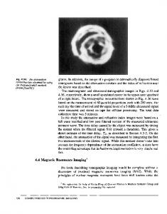
Fig. 1: Basic interaction processes occuring in magnetic resonance. The middle column shows in a schematic way (A) a single spin interacting with an external classical field, (B) the near field and the far field generated by an rf coil, (C) spin dipole-dipole interaction, and (D) a level diagram associated with spin-lattice relaxation. The diagrams in the right column represent Feynman diagrams for the corresponding QED elementary processes.
13
diagrams to provide a correspondence between situations familiar from the semiclassical point of view of magnetic resonance and the associated QED view. Feynman diagrams are symbolic representations of rigorous mathematical expressions. Apart from that, at the same time they provide some kind of intuitive picture of the elementary interaction processes for which they stand. Without going into any details now – we will treat some of them in later sections – let us briefly discuss the basic phenomena illustrated in Fig. 1. The first one, Fig. 1 (A), represents the interaction of a spin-1/2 particle with an external electromagnetic field. The source of the field might be unspecified or it might be explicitly given (e.g., a current in a coil). In the corresponding Feynman diagram, for example the diagram (a) in Fig. 1 (A), we draw a line with an arrow to represent the spin particle. This directed line enters a vertex, where the discrete “interaction event” occurs, here it is the emission or absorption of a virtual photon, symbolized by a wavy line. After the interaction event the spin particle is left in a state (drawn by an outgoing line with arrow) different from the initial state. Virtual photon exchange happens between the spin particle and the (nonspecified) external source of the electromagnetic field. We may add more details to this process by explicitly specifying the external source current (diagram (b)). In that case the virtual photon exchange affects both interaction partners, the current density that corresponds to the spin particle (sec. 6) and the current density that represents the external source. The two diagrams (a,b) provide the basis to appreciate the concept of the “single-spin free induction decay” and the basic mechanism of NMR radiation damping, both treated in sec. 8. Fig. 1 (B) offers a glance to more details when a spin particle interacts with an rf field, for example, during the application of an rf pulse. Classically the rf current in a coil or circuit generates an electromagnetic field that interacts with the spin inside or nearby the coil. We call this field the near field, characterized by a distance to the source (the current in the coil wire) small compared to one wavelength. A free standing coil (that means a coil not completely surrounded by a shield) also generates an rf field at larger distances (one wavelength and more) which is the far field. In Fig. 1(B) in the center, the graphical plot on top shows a snapshot of the rf far field magnitude |B| generated by an rf current in a solenoidal coil (6 turns, pitch angle , limit radius r0, cf. ref. (87)) located in the center of the field distribution. Taking the center part of that field distribution (field of view magnified by a factor of 5), we see the near field close to the coil. Under the QED point of view, we may interpret the interaction between spin and near field as virtual photon exchange while the far field arises from those photons that, for example, are emitted by the rf current and that are not absorbed within a given time interval, thus they are asymptotically free photons. This principal situation is shown by the Feynman diagram in Fig. 1 (B), more details will be treated in secs. 5 and 7. Likewise, direct dipole-dipole interaction, a specific example for a spin-spin interaction illustrated in Fig. 1(C) can be understood as virtual photon exchange. Finally, even spinlattice relaxation (characterized by the time constant T1) can be cast into the QED language, Fig. 1 (D). Every transition of a spin between Zeeman levels corresponds to a virtual photon exchange between the spin particle and the lattice-degrees of freedom, where the lattice represents a partner for the interaction with a stochastic or statistically fluctuating current density, resulting from the
14
stochastic motion , e.g., of molecules in a liquid. In a similar way, spin-spin relaxation could be treated.
In the present paper we focus on the basic interactions exemplified in Fig. 1 (A) and (B), i.e., we deal with the interaction of a single spin (or more than one, but then isolated spins) with the static field and with an rf field or microwave field and we provide a QED explanation of the electromotive force induced in a coil or circuit by a single spin. We will call that “single-spin FID”, although an FID of a macroscopic sample contains more features, for example, the dephasing of magnetization originating from many spins with slight resonance offsets, spin-spin relaxation, explicit spin-spin couplings, etc. These latter phenomena are not treated in the present article. On the other hand, NMR radiation damping – to be understood as the back action of the rf current generated by the electromagnetic field originating from the spin particle – also appears when only one spin is present. Admittedly, this effect is extremely small and “hard to measure” for a single spin. So the scope of the present paper might be summarized as treating the basic and elementary interaction
processes relevant for magnetic
resonance, like virtual photon exchange and emission of asymptotically free photons. These elementary processes could be used as building blocks to deal with more complex situations in bulk samples including multi-spin systems characterized by interactions between like spins and unlike spins, spin-lattice relaxation and spin-spin relaxation.
In order to finally achieve the proximity to magnetic resonance phenomena in the form as we know it from the NMR and ESR spectroscopy literature, we meet approximations and assumptions: first, we start with the simple classical expression of Coulomb interaction energy and generalize this step by step to arrive at a covariant expression for the Feynman propagator. After analyzing it and deriving the associated concepts of virtual photons and asymptotically free photons (secs. 3 and 4) we introduce a photon scattering model for pulsed NMR (sec. 5). Here we treat the current densities as non-operator quantities, which is allowed when we would treat the spin particles either as classical or when we treat them as quantum objects, in the latter case in first quantization (with the wave function as a function). For the spin particles we perform the transition to the nonrelativistic realm (slow velocities, low energies, low momenta). Thus three cornerstone assumptions are involved: (a) the electromagnetic field is assumed to be a relativistic quantity (expressed by the associated Feynman propagator), (b) initially the spin current density is introduced as a covariant quantity, however for the spin particles we apply the nonrelativistic approximation (i.e., small velocities, small energies, small momenta), see secs. 5 and 6, and finally (c) we consider the spin particles as quantum objects (with a spatial and spin wave function) with the result that the spin current density is also a function (no second quantization of the fermion field). We start with (a) in deriving the Feynman propagator.
15
3. THE FEYNMAN PROPAGATOR. As indicated in the introduction, we must create some formal basis to fully appreciate the concept of virtual photons. For edifying reasons let us begin with an almost tautological definition of the term interaction. Two partners (particles, fields, etc.) are interacting with each other when partner 1 acts upon partner 2 and partner 2 also acts upon partner 1. So we may explain interaction by reducing it to the concept of action. In physics, the quantity of action is defined as the time integral over the Lagrange function L. In classical mechanics, the Lagrange function is given by the difference of kinetic and potential energy of particles. The potential energy term constitutes the interaction of the particle with either an external field or with an interaction partner. If for the moment we disregard kinetic energy and turn to field theory, the Lagrange function for the interaction becomes (up to a sign) equal to the interaction Hamiltonian or interaction energy. Therefore, we will start our discourse by discussing a stepwise generalisation of formal expressions for the electromagnetic interaction energy and then turn to the quantity of action associated with it. We begin by considering two point charges Q1 and Q2 at distance r. The electrostatic interaction energy reads
EQ
Q1Q2 4 0 r 1
[1]
where 0 denotes the dielectric permittivity of the vacuum and r is equal to the distance between the two charges Q1 and Q2. The Coulomb interaction energy EQ can take positive or negative values, depending on the signs of Q1 and Q2, where for opposite charges, i.e., attractive forces, we get EQ < 0. We make a first step towards generalization by not assuming point charges, but electric charge densities 1 (x) and 2 (y ) distributed in space given by the position vectors x and y with
r | x y | . Thus
EQ
1 4 0
d x d 3
3
y
1 (x) 2 (y ) r
[2]
where now two integrals appear over the three-dimensional volumes with volume elements d 3x and d3y occupied by elements of the charge densities 1 (x) and 2 (y ) , respectively. A similar expression can be written down for the interaction energy of two electromagnetic currents or current densities j1(x) and j2(x):
EC
0 3 j (x) j2 (y ) d x d 3 y 1 4 r
[3]
with µ0 being equal to the magnetic permeability of the vacuum. We may also admit charge and current densities that explicitly depend on time and, for generality, we may assume that charge
16
distributions as well as current distributions are present simultaneously. The total interaction energy reads
1
1 (x, t ) 2 (y, t ) 0 j1 (x, t ) j2 (y, t ) 1 3 3 0 EI d x d y 4 r 2 c 1 (x, t ) 2 (y, t ) j1 (x, t ) j2 (y, t ) 0 d 3 x d 3 y 4 r
[4]
where c2 = 1/0 µ0 . Let us introduce the 4-position vector x m (ct , x) including time and space coordinates, where the superscript m counts the components, with m = 0 for the time coordinate (multiplied by the speed of light c), x0 = ct, and m = 1,2,3 referring to the three spatial components of the vector x. Likewise, let us merge the scalar charge density (x) and the vector current density
j(x) into a single 4-vector j m ( c, j) and refer to it as the 4-current density. For more details on the definition of 4-vectors in Minkowski space-time, we refer to Appendix A. In Eq. [4] let us drop the subscripts 1 and 2 labelling the charge and density distributions because we recognize that the space-time coordinates x and y distinguish them already. So Eq. [4] appears in the concise form
EI
0 3 j m ( x) jm ( y ) 3 d x d y 4 r
[5]
with the scalar product, j m ( x) jm ( y) j 0 ( x) j0 ( y) j( x) j( y) , in Minkowski space-time. Note, in expressions like ambm we apply the sum convention: ambm a0b0 – (a1b1 + a2b2 + a3b3) (see Appendix A).
We recognize that until now we have made no explicit assumptions about how fast the interaction may propagate between jm(x) and jm(y) – in fact, in Eq. [5] we implicitly assumed that the interaction propagates infinitely fast. This becomes more obvious if we rewrite Eq. [5] as
EI
m 0 0 0 3 3 0 j ( x) ( x y ) j m ( y ) d x d y dy 4 r
[6]
where we have inserted Dirac’s function with the time difference x0-y0 as an argument and an additional integral over the time coordinate y0. Integrating the whole expression in [6] over dy0 along the entire time axis, we come back to Eq. [5]. Alternatively, we could have performed the time integral also over dx0 instead of dy0, with the same result. In other words, the time coordinates appearing in jm(x) and in jm(y) are equal, x0 = y0, as dictated by the function – the interaction occurs instantaneously
17
As stated earlier, the Lagrange function L for the interaction equals the interaction Hamiltonian or interaction energy EI up to a sign, i.e., we have L = – EI . Furthermore, the time integral over L is equal to the action functional W1 for the interaction considered:
W1
dx 0 1 j m ( x) ( x 0 y 0 ) jm ( y) L dx 0 EI 0 dx 0 d 3 x d 3 y dy 0 c c 4 c r
[7]
A few words to explain what is meant by action functional. A functional is a mapping that assigns a number to a function or to a vector of functions (likewise, a function assigns numbers to numbers or to a vector of numbers). In the case of the action functional [7], we have the function jm(x)(x0-y0) jm(y) / r. Integrating over the full range of all the variables (i.e., entire time dimension and entire space) assigns a number, W1 to the vector of two functions j(x) and j(y). Now from Eq. [7] on we are not concerned with interaction energy anymore, but more generally with the action related to the interaction. The integrals over the time intervals dx0 and the three-dimensional volume elements d 3x can be formally assembled together as one integral over the space-time element d4x. Likewise the same can be achieved for the time intervals dy0 and volume elements d3y to obtain d4y. Hence, the action functional [7] can be written with two space-time integrals as
W1
0 j m ( x) ( x 0 y 0 ) j m ( y ) 4 4 d x d y 4 c r
[8]
Now we introduce, for physical reasons, the requirement that any action from jm(x) to jm(y), or vice versa (thus, interaction), can only be a retarded action, i.e., it takes a certain time to propagate from one region in ordinary space to another one at distance r. When this propagation occurs with the speed of light, c, the time interval for propagation is equal to r/c. We can easily modify Eq. [8] to take into account retardation by modifying the argument of the function accordingly:
0 j m ( x) (( x 0 y 0 ) r ) jm ( y ) 4 4 W1 d x d y 4 c r
[9]
With Eq. [9] we have obtained a first remarkable result. In order to see this, let us define the function
ret ( x y )
0 (( x 0 y 0 ) r ) , r |xy| 4 c r 18
[10]
such that the action W1 can be written as
W1 d 4 x d 4 y j m ( x) ret ( x y) jm ( y) d 4 x j m ( x) AmR ( x) and where we have implemented the retarded potential ARm(x) generated by the current jm(y),
AmR ( x) d 4 y ret ( x y ) jm ( y ) d 3 y dy0
0 (( x 0 y 0 ) r ) jm ( y ) 4 c r
j ( x r, y) 0 d3y m 0 4 c r
[11]
as the convolution integral of ret(x-y) with the current density jm(y). The kernel of the first integral in Eq. [11], ret(x-y), is referred to as the retarded Green function associated with the inhomogeneous wave equation. It is also called the retarded propagator (see Appendix B).
After having introduced retarded action, returning to Eq. [9], let us perform the next step: we consider the time ordering of events. In Eq. [9] we have done so already in an implicit way by expressing retardation through the function with the argument (x0-y0) - r . Because r is strictly positive, the integrals in [9] are nonzero if and only if x0 - y0 > 0, which means x0 > y0 : the event at time instant y0 (for example, a change of the current density element located in space position y ) is earlier than the event at time x0 (when the field change caused by the previous current density change arrives at the current density element in space position x) – the cause precedes its action. In general, when we talk about interaction, we have to admit that, in principle, also the inverse time order may happen in conjunction with an exchange of the two positions in space, i.e., an event at position x happens first at time x0, the field change travels to position y where it arrives at a later time y0 such that, as causality dictates again, we have x0 < y0 . Since both event orders are allowed, the total action is given as the arithmetically weighted sum of both:
W
W1 W2 j m ( x)[ (( x 0 y 0 ) r ) (( x 0 y 0 ) r )] jm ( y) 0 d 4 x d 4 y 2 4 c 2r
[12]
The first function on the right-hand side of Eq.[12] stands for the time order x0 – y0 > 0, while the second one takes the reverse order into account, x0 – y0 < 0. The fact that both time orders must appear is almost trivial for an interaction. j(y) acts on j(x), so x0 – y0 > 0 as well as j(x) acts on j(y), hence we have x0 – y0 < 0. We may depict this diagrammatically as shown in Fig. 2. The two interacting current
19
densities are drawn as lines with arrows, the interaction between them as a wavy line. In the diagrams the time axis points into vertical upward direction and Figs. 2a and 2b correspond to the two time orderings as explained above. In Fig. 2 we have drawn second-order Feynman diagrams symbolizing
Fig. 2: Diagrammatic representation of the interaction between two currents, (a) where j(y) acts on j(x) and (b) vice versa, j(x) acts on j(y), representing two opposite time orderings. The current densities are drawn as lines with arrows, the electromagnetic interaction between them as wavy lines. The diagrams shown represent two examples of second-order Feynman diagrams.
the elementary electromagnetic interaction process occuring between two electromagnetic current densities. A systematic introduction into general Feynman diagrammatic techniques can be found, for example, in references (81, 89, 90, 124). We observe that the function is even, i.e., it holds
(( x0 y 0 ) r ) (( x0 y 0 ) r )
[13]
such that Eq. [12] formally appears to be the sum of a time-retarded and a time-advanced part. As we have discussed above, the latter just reflects the alternative time ordering (which always takes place together with an exchange of spatial coordinates) that we have to admit in interaction processes. The time-advanced part does not indicate a violation of causality nor does it describe noncausal evolution backards in time, although formally, sometimes in the literature, it is termed anticausal. So the action functional for the electromagnetic interaction of two current densities reads
W1 W2 0 j m ( x)[ (( x0 y 0 ) r ) (( x 0 y 0 ) r )] jm ( y ) 4 4 W d x d y 2 4 c 2r
20
[14]
The difference between Eqs. [9] and [14] is that in Eq. [9] only one fixed time order is taken into account, while Eq. [14] is more general, because it also allows the reverse order when simultaneously the space coordinates are reversed. Both time orders correspond to retarded action. From now on, for the sake of simplicity in notation, we adopt Heaviside-Lorentz units (which are characterized by setting 0 = 1 and 0 = 1) and, in addition, we also set c = 1, = 1. In the resulting system of physical units it then appears that energy, mass, linear momentum, wavenumber, and frequency have the same unit: 1/meter. The corresponding units in SI are obtained by multiplying accordingly with c and/or , the SI units for the field quantities by re-introducing 0 and 0 accordingly (78). We take a look at the formal Fourier decomposition of the function,
( x0 )
1 2
exp(i x ) d , 0
[15]
which tells us that, upon integration, it contains positive as well as negative frequencies . As it will turn out, for the case of the quantized electromagnetic field these frequencies correspond to energies for photons.
Again for physical reasons, anticipating the photon picture that we will adopt when we turn to QED, we require that is strictly positive or zero, not negative. This is equivalent to admitting only positive (or zero) energy values carried by a single photon. In order to take this requirement into account, we have to restrict the integration range in Eq. [15] to run over values only from 0 to instead of the full range of – to
such that we arrive at the modified function defined by the “half-sided”
Fourier integral (note here, by definition, the different pre-factor 1/42)
(x0 )
1 4
2
exp(i x
0
)d
[16]
0
We will investigate the detailed properties of + later in sec. 4 (see also Appendix C). For the moment it may suffice to say that the features of + are central to the mathematical description of photons appearing in interaction processes. One remark in advance: while Dirac’s function can be considered as a real-valued generalized function, i.e., its arguments are on the real line and the values of are, loosely speaking, either zero or infinite, but real-valued, this “real-valuedness” is not the case anymore for +. So the requirement of positivity for the photon energy with the consequence of
21
the restricted integration range in Eq. [16] leads to a phenomenon called time dispersion: + becomes complex-valued (with a real and an imaginary part). In order to understand the consequences, let us rapidly anticipate some of the steps that lead into QED, more thoroughly discussed in later sections. The positivity requirement for the energy of photons, exchanged between the current densities, has farreaching implications. First, the quantity of action, W, becomes a complex-valued quantity. Second, with the probability amplitude Z in QED (22) defined as
Z = exp(iW)
[17]
for the photon propagation in QED, the resulting probability for a photon propagating from one current to the other current is equal to |Z|2. Thus if W is real, we get |Z|2 = 1 and if W appears to have an imaginary part, we see that |Z|2 < 1. The latter statement means that not every photon emission leads necessarily to photon re-absorption – there is a finite probability that photons “break free”. We will discuss that in more detail in sections 4 and 5. So if we modify Eq. [14] by replacing by + , we arrive at
j m ( x)[ (( x 0 y 0 ) r ) (( x 0 y 0 ) r )] j m ( y) 1 4 4 . W 2 d x d y 4 2r where the additional factor 2 in front of the two space-time integrals takes into account the different prefactor in Eq. [16] as compared to the pre-factor in Eq. [15]. The following identities hold (see Appendix C)
(( x 0 y 0 ) r ) (( x 0 y 0 ) r )
(( x 0 y 0 ) 2 r 2 ) (( x y ) 2 )
2r (( x y ) r ) (( x 0 y 0 ) r ) (( x 0 y 0 ) 2 r 2 ) (( x y ) 2 ) 2r 0
0
[18]
where (x – y)2 is equal to the squared 4-distance between the two space-time points of the elementary interaction events, i.e., ( x y)2 ( x0 y 0 ) | x y |2 ( x0 y 0 ) r 2 . When
introducing [18], the
expression for the electromagnetic action functional reads
W
1 4 d x d 4 y j m ( x) (( x y) 2 ) j m ( y) 2
Let us introduce
22
[19]
DFmn ( x) g mn ( x 2 ) ,
[20]
where gmn designates the metric tensor (cf. Appendix A) and refer to DF as Feynman propagator or Feynman-Green function for the electromagnetic interaction. Similar to the retarded propagator ret defined by Eq. [10], the Feynman propagator DF is a further Green function associated with the wave equation (Appendix B). With the definition [20], the action functional [19] can be written as
W
1 4 d x d 4 y j n ( x) DFmn ( x y) j m ( y) . 2
[21]
The expression [21] states that the electromagnetic action (interaction) between two current densities jn(x) and jm(y) is mediated by the Feynman propagator DF(x – y) for the electromagnetic field. We remark that [21] is quite general, however it can be specialized for the case of spin-spin interactions as well as for interactions between spins and resonator, by specifying the current densities accordingly. There is no principal restriction for the current density: it can represent a spin current density or a current density due to electron conductivity, microscopic or macroscopic. We will turn to that subject in more detail in sec. 6. In analogy to the retarded potential, Eq. [11], the integral over d4y is equal to the 4-potential An(x) at space-time point or region x generated by the current density jm(y) at spacetime point or region y,
An ( x) d 4 y DFmn ( x y) jm ( y) .
[22]
Hence
W
1 4 d x j n ( x) A n ( x) 2
[23]
In summary, we have started our discussion with the classical expression for the interaction energy for two interacting current densities and introduced (a) time retardation, (b) time ordering of events, and (c) positivity of the energy exchanged as a quantum between the interaction partners. As a result we obtain the Feynman propagator DF for the electromagnetic field. So far we are still (almost) within the scope of classical electrodynamics including special relativity (retarded field propagation with finite speed). We have not yet properly quantized the electromagnetic field. In doing so in the next section, we will find an interpretation for DF in physical terms. The general result [21] remains valid in a quantized field theory. Focusing on magnetic resonance, it becomes necessary to specify the general current densities jm for spins and/or electric currents. We will accomplish that in sec. 6.
23
4. QUANTIZATION OF THE ELECTROMAGNETIC INTERACTION FIELD. VIRTUAL PHOTONS.
Quantization of the electromagnetic field involves two formal ingredients. First (a) the field functions Am(x), i.e., the 4-vector potential Am ( x) ( A0 ( x), A( x)) including the scalar potential A0(x) = /c and the vector potential A(x), become field operators. Furthermore (b), generally, these field operators are subject to certain commutation or anticommutation relations that determine the basic nature of the quantum field. This procedure related to these two cornerstones (a) and (b) is called canonical quantization and will be the basis for our attempt to discover virtual photons in magnetic resonance. From a practical point of view it is advantageous to begin with the classical Fourier expansion of the field functions (4-potentials) in three-dimensional momentum space (k space), reading
Am ( x)
Here
d 3k
2 2k 3
(k )a (k ) e 3
0
( ) m
( )
ikx
a ( ) (k ) eikx
[24]
k k m (k 0 , k ) denotes the contravariant 4-momentum vector (see Appendix A) with k0
proportional to the energy variable ck 0 of the field mode k and k equal to the usual wavenumber vector such that k is equal to the 3-momentum. In space-time there are generally four different polarization vectors m( ) (k ) ( 0( ) (k ), ε ( ) (k )) , enumerated by the superscript = 0,1,2,3. The Fourier coefficient a ( ) (k ) and its conjugate complex a ( ) (k ) are functions of the 3-momentum k.
The exponentials exp( ikx) contain the 4-scalar product kx k m xm (k 0 , k )( x0 ,x)T k 0 x0 k x . Summation over all polarization directions and integration over k-space yields the 4-vector Am(x) as a function of space coordinate vector x and time coordinate x0. Converting the field functions Am(x) into operators leads us to ask which of the constituents in the integral expression [24] takes over the operator role. This role is filled by the Fourier coefficients a ( ) (k ) and a ( ) (k ) , that are required to satisfy the following canonical commutation relationships (CCR):
[a( ) (k ), a( ) (k ' )] g 3 (k k ' ),
, 0,1,2,3
[25]
with all other combinations of elements in the commutator brackets different from those in [25] yielding zero. Thus with [24] being read as a Fourier expansion of field operators and with the Fourier coefficients required to satisfy the CCR [25], we have performed the formal task of quantizing the electromagnetic field. This allows us to calculate commutators of field operators, [Am(x),An(y)], or
24
products of field operators Am(x)An(y), etc. We may define the Lagrangian density for the free or the interacting electromagnetic field and obtain the associated Hamiltonian (79-82), which for the free field turns out to be identical in form with the Hamiltonian for a system of harmonic oscillators. As explained in texts on quantum field theory and quantum electrodynamics, the operators a ( ) (k ) and
a ( ) (k ) reveal themselves as annihilation and creation operators for photons, the quanta of the electromagnetic field.
Suppose there is a state | 0 > of the electromagnetic field with no photons present in the field, also called the ground state or the vacuum state of the field and define
a( ) (k ) | 0 0, a( ) (k ) | 0 | 1
[26]
where | 1 > denotes a state of the field with exactly one photon present with momentum k and polarization ( ) (k ) . We may generalize this for n photons,
a( ) (k ) | n n | n 1 , a( ) (k ) | n n 1 | n 1
[27]
Applying a ( ) (k ) and subsequently a ( ) (k ) to the field state | n > we obtain from [27]:
a( ) (k )a( ) (k ) | n n | n
[28]
which qualifies the product operator a( ) (k ) a( ) (k ) as the photon number operator. The field states | n > with a precisely defined number n of photons in a given mode (, k) are eigenstates of the photon number operator and are called Fock states. These form an orthonormal basis set of states in a state space called Fock space, a specific example of an infinite-dimensional Hilbert space. We mentioned the Fock states in the introduction when discussing the uncertainty relation of field amplitude and phase and we maintained already that Fock states cannot correspond to states of the electromagnetic field in the classical limit.
In quantum field theory it makes a difference whether we say that the field contains zero photons, i.e., it is in its vacuum state | 0 >, or we say that there is no field. In the latter case, there is nothing to talk about, in the former case, there is quite a bit to discuss. We may calculate expectation values of operators with field states to be compared with measurements, so for example we might be interested in vacuum expectation values. Interestingly, we find for instance,
25
0 | Am ( x) | 0 0,
0 | Am ( x) An ( y) | 0 0 .
[29]
which can be easily verified when taking into account Eqs. [24-26]. While the vacuum expectation value of the field operators vanishes (likewise this is also true for the vacuum expectation values of the electric field and the magnetic induction field calculated from Am(x)), it is not the case for the vacuum expectation value of higher order products. Thus, the variance, or two-point correlation, or fluctuation amplitude of field quantities can be nonzero in the vacuum state – a typical situation occuring in quantum field theory.
We return to the discussion we began in the previous section concerning the two current densities interacting with each other, i.e., the current density jn(x) generating the field An(y) at the space-time position y of the current density jm(y) and vice versa, the current density jm(y) producing the field Am(x) at the space-time position x of the current density jn(x). The interaction of the two current densities has been expressed by Eq. [21]. But consider the following: instead of correlating the two current densities in that way, we can also correlate the two associated fields by forming the product Am(x)An(y) and calculating expectation values for given field states – the simplest and most straightforward would be the vacuum expectation value. Moreover, because we saw in the previous section that time ordering is essential in describing interactions to ensure causal behavior, we may include that in our field correlation and calculate not just < 0 |Am(x)An(y) | 0 > , but calculate the timeordered vacuum expectation value < 0 | T(Am(x)An(y)) | 0 >, where Dyson’s time ordering operator T has been introduced, defined as
A m ( x) A n ( y ), T ( A m ( x) A n ( y )) n m A ( y ) A ( x),
x0 y0 y0 x0 [30]
( x0 y 0 ) A m ( x) A n ( y ) ( y 0 x0 ) A n ( y ) A m ( x) denotes the Heaviside step function defined as (x0 – y0) = 1 for x0 – y0 > 0 and zero otherwise. We have now all the means available to calculate < 0 |T(Am(x)An(y)) | 0 >. As shown in detail in Appendix C, this calculation yields
0 | T ( Am ( x) An ( y)) | 0 iDFmn ( x y) ig mn (( x y) 2 )
[31]
Thus we find that for a quantized electromagnetic interaction field the Feynman propagator equals (up to a constant prefactor) the vacuum expectation value of the time-ordered field operator product Am(x)An(y), that is, the Feynman propagator corresponds to the two-point vacuum field correlation function. Note, the correlation here includes time and space correlation – we are in space-time.
26
Reading the expression [31] as a space-time two-point correlation function opens up the possibility of an even more extended interpretation of the Feynman propagator DF. First we observe that when we insert the expansion [24] for the field operators into the expression for the vacuum expectation value of the time-ordered field operator product, 0 | T ( Am ( x) An ( y))) | 0 , terms like
0 | T (a ( ) (k )e ikx a ( ) (k )eikx )(a ( ) (k )e iky a ( ) (k )e iky ) | 0 ( )
0 | T a (k ) e
ik ( x y )
a
( )
[32]
(k ) | 0
appear. The last line in [32] may be read from right to left as follows: initially there is the photon vacuum | 0 >. The creation operator a ( ) (k ) creates the single-photon state | 1 a( ) (k ) | 0 . As indicated by the time ordering and the exponential function e-ik(x-y), the photon propagates (assuming y0 < x0) from y to x. At space-time point x the annihilation operator a ( ) (k ) annihilates the single-photon state again, which leaves the field in the vacuum state: | 0 a ( ) (k ) | 1 .
Fig. 3: Pictorial representation of the photon propagator with explicit time ordering according to Eq.[30]. For x0 < y0 the photon is created in space-time point x and propagates to space-time point y where it is annihilated (right diagram). For y 0 < x0 the photon is created in y and propagates to x where it is annihilated (left diagram).
27
The process of creating a photon in y, letting it propagate to x, then annihilating that photon in x, appears in a time-ordered fashion – i.e., the photon is first created at time y0, and then later at time x0 it is annihilated (left side of Fig. 3) – formally this is taken care of by the time-ordering operator T. For the case x0 < y0 (right diagram in Fig. 3) the photon is created in x, propagates to y where it is annihilated again. The photon only exists while propagating from y to x (or from x to y when the time order is reversed), the initial and final field states are photon vacuum states. It is for that reason that the intermediate single-photon state, | 1 a( ) (k ) | 0 , appearing here is referred to as occupied with a virtual photon. Virtual photons emerge as intermediate states between the initial and final photon vacuum state. Therefore the Feynman propagator, also referred to as the photon propagator, represents the mathematical vehicle describing virtual photons. With Eq. [31] we could set up a new expression for the action functional W , Eq. [21], which now has also a new interpretation for the probability amplitude Z = exp(iW), Eq. [17], that governs the probability |Z|2 for the photon propagation between the site of emission and the site of absorption. Photons are being exchanged with probability |Z|2 1. Photon propagation is thus not a deterministic process, it exhibits some uncertainty measure expressed by |Z|2 admitting the possibility that an actual photon exchange happens, as illustrated in Fig. 3, emission and subsequent reabsorption (the appearance of a virtual photon) as well as admitting the possibility that photons emitted are not reabsorbed or photons absorbed have not been emitted in the past.
In the scheme drawn here it seems that the virtual photon apparently emerges out of nothing and disappears into nothingness. This is, of course, not the case, we just have isolated the interaction part – interaction occurs between two current densities jm(x) and jn(y) and the diagrams in Fig. 3 can be seen as subdiagrams contained in the diagrams of Fig. 2. So it is more appropriate to say that virtual photons are emitted by one current density and reabsorbed by another (or the same) current density. Emission of virtual photons changes the state of the particles that constitute the current density, likewise the reabsorption of virtual photons. In Fig. 2 we have indicated that by a kink in the lines symbolizing the current densities, appearing when emission or absorption occurs. The particles that compose the current densities in Eq. [20] might be conduction electrons in a piece of metal wire being a part of a coil, or it might be a spin particle in a specific spin state.
The photon propagator governs the electromagnetic interaction between current densities. In order to see this, we must turn back to Eqs. [20] and [31] and further analyze the distribution (( x y)2 ) , an essential constituent of the Feynman propagator DF(x-y) and arising from Eq. [31]. As shown in lengthy detail in Appendix C (see, Eqs. [C8] to [C17]), DF(x-y) turns out to be,
28
DFmn ( x y ) g mn (( x y ) 2 )
g mn 1 (( x y) 2 ) i 2 2 4 ( x y )
[33]
As already mentioned in sec. 3 when introducing the probability amplitude Z (Eq.[17]), we observe in Eq. [33] that DF(x-y) is complex-valued; it consists of a real part, given by Dirac’s distribution, and of an imaginary part, given by Cauchy’s principal value distribution (1/(x-y)2) . The appearance of both is elaborated in Appendix C (see Eqs. [C1-C7]). As a preliminary and very crude exposition, we can say that the distribution represents a singular function that is zero everywhere except where its argument is equal to zero – there it is divergent. The Cauchy principal value distribution (1/(x-y)2) behaves like the function 1/(x-y)2, for (x-y)2 approaching 0 it is also divergent. We have to suspect, that such singular “functions” are not simply functions in the ordinary sense, their singular behavior and other features warrant a whole mathematical theory – their treatment is part of the theory of distributions as introduced by Schwartz (83) (see also refs. (84, 85)). It would be far outside the scope of the present article to elaborate on this theory here; we will only pick those bits and pieces necessary to formulate the photon propagator and other Green functions. Functions or distributions with singularities are only one kind of infinity or divergence characteristic of quantum electrodynamics or, more generally, of quantum field theories. In QED, expressions that reveal divergent behavior can be submitted to procedures called renormalization or regularization, which allow us to calculate expectation values for physical quantities like energy, linear momentum, angular momentum, and others, which then turn out to be finite. One relatively simple example for such a regularization procedure, the “taming” of the singularities of (x) and (1/x), is carried out in Appendix C.
In four-dimensional k space, the Fourier domain of space-time, we find for the photon propagator (see Appendix C, Eq. [C14]),
1 g mn g mn 2 i (k 2 ) 0 k 2 i k
DFmn (k ) lim
[34]
In Eq. [34] we recognize, comparing it with Eq. [33], that the and distribution exchange their roles as far as the real and imaginary parts are concerned. We stress the point: Eqs. [33] and [34] represent the central result of this section and will provide us with the key characteristics for virtual photons.
For our following discussion of Eqs. [33] and [34] it is worthwile to introduce two technical concepts: (a) the concept of a lightcone in space-time and (b) the concept of a mass shell in momentum space. The technical definition of the notions of a lightcone and a mass shell is given in Appendix A (in particular, see Figs. A1 and A2), where it is shown that a 4-vector u given in space-time can be one of
29
three kinds, depending on its norm-square u2. If u2 is positive, then vector u is referred to as time-like. For coordinate vectors x this means x 2 c 2 t 2 r 2 0 , from which follows c 2 t 2 r 2 . In other words, time-like coordinate vectors in space-time refer to propagation over distances r with a propagation speed below the speed of light, c, i.e. subluminal propagation, where r < c|t|. These vectors refer to points inside a region in space-time that forms a double cone with its apex at the coordinate origin (Fig. A1). There are time-like vectors in the forward cone for which t > 0 and in the backward cone for t < 0. Furthermore, there are vectors u in space-time, called space-like vectors, for which u2 < 0 holds. For coordinate vectors this becomes
x 2 c 2 t 2 r 2 0 , consequently
c 2 t 2 r 2 , referring to superluminal propagation. Finally there are vectors u with u2 = 0, called light-like vectors. Coordinate vectors x with x2 = 0 are precisely those vectors that lie on the surface of the lightcone and it holds c 2 t 2 r 2 , i.e., propagation with luminal speed c.
The k space is characterized by the same metric properties as space-time. Thus the Fourier domain of the time dimension x0 = ct becomes the k0 dimension, which is frequency or energy. Likewise, the three spatial dimensions needed to specify a three-dimensional position vector x have their Fourier domain counterpart in three k space dimensions with the momentum vector k. The relationship k2 = 0, or equivalently 2 c / with frequency and wavelength of a freely propagating electromagnetic wave or free photons (see Appendix A, Eqs. [A11, A12]) defines a spherical shell with radius k0 (Appendix A, Fig. A2) in 3-momentum space. Those photons that satisfy the energymomentum relationship k2 = 0 are called on-shell, otherwise off-shell. Likewise, photons that travel exactly on the surface of the lightcone are called to be on the lightcone, otherwise off the lightcone.
Now let us examine in detail the expressions in Eqs. [33] and [34]. In Eq. [33] we have the sum of two terms. The first term contains ((x-y)2), which means that it contributes only for (x – y)2 = 0, (where Dirac’s function becomes singular) to integrals like [21] or [22], i.e., the space-time difference vector x – y is light-like, hence it describes propagation of photons on the lightcone, propagation with the speed of light, c. The second term in Eq. [33] constitutes Cauchy’s principal value (1/((x – y)2)). This distribution is singular for (x – y)2 = 0 (i.e., on the lightcone), but it is also different from zero for (x – y)2 < 0 as well as for (x – y)2 > 0, i.e., for time-like as well as for space-like distances x-y in space-time. Hence this term formally describes propagation off the lightcone ! Turning our attention to Eq. [34], we find again two terms: (k2) contributing only for k2 = 0, i.e., corresponding to photons on-shell, and
(1/k2) being
singular for
k2 = 0, but
contributing for k2 0 as well, hence allowing photons to be off-shell. We also recognize that in Eq.[33] the real part of the photon propagator, Re(DF(x-y)), contains ((x – y)2) while the imaginary part, Im(DF(x-y)), contains (1/((x – y)2)). In momentum space it is just the other way around, Re(DF(k)) gives (1/(k2)) while Im(DF(k)) contains (k2).
30
Fig. 4: Pictorial illustration of the Fourier transform relationships as expressed in Eqs. [33, 34] and Tab. 1. The real part of DF(x) characterizes propagation strictly on the lightcone indicated by a sharply drawn lightcone surface, corresponding to off-shell positioning in k space, as given by the real part of DF(k), symbolically indicated by a sphere with fuzzy surface. Likewise, off-lightcone propagation described by the imaginary part of DF(x) is illustrated by an unsharp lightcone, and on-shell positioning as given by the imaginary part of DF(k) pictured by a k sphere in 3D momentum space with sharp radius k0. Re(DF(x)) and Re (DF(k)) are Fourier transforms of each other. The same holds for Im(DF(x)) and Im(DF(k)) also forming a Fourier transform pair.
Table 1: Characteristics of the real and imaginary parts of the Feynman-Green function in space-time and k space representation and their interpretation in terms of virtual and asymptotically free photons.
Feynman-Green function DF Minkowski space-time, coordinates x, y 4-dim. momentum space, Coordinates k Interpretation
Associated solution of the wave equation
real part of DF
imaginary part of DF
1 (( x y ) 2 ) 4
+
does propagate on the lightcone 2
+( 1/ k ) positioned off-shell virtual photons travel on the lightcone, i.e., (x – y)2 = 0, but they may be off zero-mass shell, k 2 0. Inhomogeneous solution, interacting fields
31
1 2 2 4 ( x y) 1
may propagate off the lightcone
(k 2 ) positioned on-shell asymptotically free photons may travel off the lightcone, i.e., (x – y)2 0, but they are on zero-mass shell, k 2 = 0. Homogeneous solution, free fields
These findings are illustrated in Fig. 4. In this figure propagation on the lightcone (with ((x – y)2)) is symbolized by a sharply drawn diagram. In contrast, propagation off the lightcone (characterized by (1/((x – y)2))) is drawn as a slightly fuzzy lightcone symbolizing that propagation may deviate from the lightcone surface. Likewise in momentum space: being off-shell (with (1/(k2))) is symbolized by a sphere with unsharp boundary, being on-shell ((k2)) by a sharply drawn sphere. We further recognize that a sharp lightcone corresponds to an unsharp momentum sphere and vice versa, a sharp momentum sphere has an unsharp lightcone as its Fourier counterpart.
We summarize these results once more in Table 1 where we also provide a first interpretation. As discussed before with Eq. [32], the photon propagator DF yields virtual photons, i.e., photons that are emitted and reabsorbed, and between these two events they propagate through space arbitrating the interaction between emitting and absorbing current densities. But now apparently we have found two kinds of photons to which we referred to in Table 1 as virtual photons and asymptotically free photons, either being on the lightcone or off the lightcone in space-time, or equivalently, being off-shell or onshell in k-space, respectively. In a general setting, the distinction of virtual photons and asymptotically free photons on the basis of analyzing Eqs. [33, 34] has been suggested in a paper by Castellani, et al., (94).
The peculiarity of two types of photons needs an
explanation that involves (i) Heisenberg’s
uncertainty relations for the virtual photon exchange and (ii) an iteration of the argument related to the imaginary part of DF(x-y) to explain the probabilistic appearance of asymptotically free photons. Ad (i) In a general setting, as regards the uncertainty relations for quantum mechanical observables expressend by (Hermitian) operators F and G acting on state functions that are elements of a Hilbert space, we have the general relationship F G (1/2) |< [F, G] > | for the standard deviations (uncertainties) F = ||(F – < F >) || and G = ||(G – < G >) || , which follows from Schwarz’ inequality valid for state functions in Hilbert space (see, e.g., ref. (98), pp. 191). The notation indicates the quantum expectation value and [F, G], as usual, denotes the commutator of the two operators F and G. The symbol |||| stands for the norm (which is a real, positive number for 0) of the state function . Hence the expression ||(F – < F >) || denotes the norm of the state function that we get as a result when applying the operator (F – < F >) to . As an example, we could take the position coordinate X (as an operator) and the operator of 3-momentum component Px and with the commutator [ X , Px ] i we arrive at the well-known positionmomentum uncertainty relation XPx / 2 .
32
If we want to apply the same “recipe” to the physical quantities energy and time in order to infer how energy and time uncertainties are related to each other, we face a serious obstacle: while energy E appears as an operator, it is the Hamiltonian of the system considered, time t is just a parameter, a coordinate in space-time. There is no time operator, neither in orthodox nonrelativistic quantum mechanics nor in quantum electrodynamics ! Nevertheless the question of the validity of an energytime uncertainty relation E / 2 is entirely reasonable as long as we can provide a physical meaning for the time interval . In order to further clarify this meaning of , let us return to the accepted uncertainty relation E G (1/2) | < [H,G] > | involving the energy uncertainty E, with G equal to an arbitrary Hermitian operator, and H equal to the Hamiltonian. Denoting by G the operator for “change of G over time”, then the equation of motion reads G (i / )[ H , G] G / t . If we suppose that G does not depend explicitly on time, then G (i / )[ H , G] and we are allowed to write
EG ( / 2) G . Now, due to Ehrenfest’s theorem (ref. (98), p. 210) it holds
G d G / dt , such that E G ( / 2) | d G / dt | . Let us define the time duration
G d G dt
[35]
which can be understood as that time interval it takes for the expectation value < G > to change in time by a value as large as the uncertainty G, or to change over time and take all values within the range G. With this definition for the time interval , it directly follows the energy-time uncertainty relation E / 2 . Now with Eq. [35] providing a meaning to the “time uncertainty” , we may claim, for example, that E x / 2 where in this case G represents the position operator X (for one dimension), further G = r is given by a distance, such that for a virtual photon propagating with velocity d G / dt d X / dt c on the lightcone we arrive at x = r/c and may interpret x as the average lifetime (the propagation time) between emission and absorption of the virtual photon with the associated energy uncertainty E. Nonetheless we emphasize, that this is just one possibility depending on the choice of the operator G = X. Alternatively we may take G = P with P equal to the 3-momentum (again in one dimension), then we obtain p = P/Fp with the force Fp equal to the total time derivative of the expectation value < P > for the momentum P. As we see here, the duration p refers to the time derivative of the expectation value of operator P and thus has a different definition and meaning as compared to x, because now it is related to the operator P instead of X. Summarizing, the time duration appearing
in the energy-time uncertainty relation
E / 2 depends on the choice of the operator G, generally noncommuting with the Hamiltonian H. For short, G specifies , see Eq. [35].
33
It should be clear by now that the question of the energy uncertainty E for a virtual photon depends on the second observable G that we may want to consider for a measurement, as an experimental boundary condition. Suppose we know the precise distance r (obtained by some measurement) between emission and absorption, the energy uncertainty for the virtual photon is equal to
E c /( 2r ) . But we keep in mind that this is only one possibility. For example, as we will investigate later in sec. 6 when looking at Larmor precession through the QED view frame, we may face the situation that, for some additional reason, E goes to zero, i.e., we may know that the virtual photon has a sharp or certain energy. For this case it follows that we are not allowed to interpret the duration as arising from a certain propagation distance r, instead we have to take p = P/Fp with the uncertainty P of the photon’s 3-momentum going towards infinity, or Fp going to zero, in such a way that still E p / 2 holds. The fact that here in our example we focus on the 3-momentum P as possibly being entirely uncertain (P becoming infinite) with an associated time interval p going towards infinity, does not contradict the situation that the virtual photon travels the propagation distance r during the time interval r/c = r on the lightcone. It is just that p r and in the case of sharp energy E the energy-time uncertainty relation has to be written down with the time interval p, not r. As we also can see, there is no contradiction with the statement that virtual photons are off-shell: the photon energy may have a sharp value, i.e., the zero-mass shell has a sharp radius, while the 3-momemtum is entirely uncertain. For a discussion on the notion of the uncertainty with respect to the Fourier transformation in relation to magnetic resonance we refer to ref. (86).
Ad (ii) As discussed earlier with Eqs. [31, 32] and with the introduction of the probability amplitude Z, the Feynman propagator as expressed in Eq. [33] also includes the transition for a photon being emitted and not being reabsorbed yet (and maybe it never will be reabsorbed) within a given time interval, or a photon being absorbed but with the uncertainty at which time it has been emitted (and, perhaps, it never was). The positivity requirement for the photon energy led to a complex-valued action functional W. The associated probability amplitude for photon propagation is equal to Z = exp(iW) where the probability character is governed by the imaginary part of W . Table 1 lists virtual photons as those which, within a given time interval x0 – y0, are emitted and reabsorbed. All other photons are asymptotically free in the sense that either emission or absorption has not taken place yet within this specified time interval. In the literature these asymptotically free photons are sometimes referred to as real photons. We prefer not to use the term “real photon” here, because in real interactions virtual photons appear to be just as real as asymptotically free photons. Nevertheless, as pointed out in expression [31], the Feynman propagator DF(x – y) as a whole characterizes the travelling path or trajectory of photons, but these trajectories appear to be “fuzzy trajectories” , the fuzziness given by the term (1/((x – y)2)), which is the imaginary part in the action functional W. This uncertainty does not only cover the trajectory between their beginning (emission) and end points (absorption), it also includes these initial and end “points” themselves. When discussing Eq. [16],
34
where we have restricted the frequency or energy range for photons to be positive (including zero), thus making a restriction in k0 space by reducing the energy value range from - … + to a smaller subrange of 0 … +, the price to pay when doing this is that we got time dispersion, the associated uncertainty is as specified by Eq. [35] . An increasing uncertainty r for the propagation time also includes the possibility that within a given time interval no emission or no reabsorption may take place. If this happens to be the case for increasingly long, or asymptotically long time intervals, then the corresponding photons are asymptotically free, either when looking towards the past (backward lightcone) or looking towards the future (forward lightcone). Thus the photon propagator DF includes or admits the possibility, that exchanging photons escape from their fate of otherwise being caught as truly virtual and going forth and back between the interaction partners. The probability for a photon to succeed in escaping to “asymptotic freedom” is different from zero and can be computed from DF and by taking the interacting current densities into account. We will perform the calculation of such an escape probability (Eq. [57]) when discussing a specific NMR probe model in the next section.
Last but not least, with the dichotomy in Table 1 we are reminded of the distinction well-known in classical electromagnetism: near field and far field. The near field is considered as the electromagnetic field in a region with distances from the source below (or small compared to) one wavelength for a given field mode. The far field is found at distances at or larger than one wavelength. There is no sharp boundary between near and far field, the transition from near to far field is gradual. Asymptotically free photons may escape to the far field, or more precisely, they may constitute the far field. Likewise, virtual photons should belong to the near field. The interpretation of virtual and asymptotically free photons outlined above will be applied to all electromagnetic phenomena discussed in the following.
From Tab. 1 we may derive a useful means of recognizing the signature of the presence of virtual photons. Apart from using the general definition that in QED virtual photons mediate the electromagnetic interaction, the following indicator points to the appearance of virtual photons: the free-photon energy-momentum relationship k2 = 0 does not hold (see Appendix A, Eq. [A10] and Fig. A2), i.e., virtual photons are off-shell. Let us review briefly some examples: (i) In structures with wave compression (which means k2 < 0) like helical waveguides or solenoidal coils (87), there it is the interaction of one part of the structure with another part of the same structure, for instance two neighboring coil turns or a space-periodic repetition of structural elements like coil turns, that signifies an exchange of virtual photons. In this sense, wave compression is understood as
/ c 2 / , i.e., we have 2 / c 2 4 2 / 2 and consequently we arrive at
2 / c2 4 2 / 2 (k 0 )2 | k |2 k 2 0 .
35
Classically we may say that the geometric boundary conditions of wave propagation are different from those in free space. Using the language of QED we may say that virtual photons, appearing because of geometric boundary conditions not present in free space, govern the wave propagation, which is different from the free space propagation characterized by asymptotically free photons. (ii) Another example where k2 0 occurs in electromagnetic fields interacting with dielectric materials. Here we encounter interactions between the electromagnetic field and the bound electric charges or electric dipoles in these materials. Macroscopically we find again wave compression: for example, a standing wave in an resonating transmission line filled with a dielectric material with r > 1 experiences a compression of its effective wavelength. (iii) Static interactions typically lead to k0 0 (see our discussion of the Larmor precession in sec. 6), i.e., the zero-mass shell degenerates to a point in k space and every photon with | k |2 0 must be virtual.
5. A QED NMR PROBE MODEL: PULSED NMR AS A SCATTERING PROCESS
In the previous two sections the basic understanding of how to interpret the Feynman-Green function, or synonymously, the photon propagator has been introduced. In the following we want to apply and illustrate the basic concepts in a model that has relevance for pulsed NMR spectroscopy. Among all the parts of an NMR spectrometer it is the NMR probe whose design is based on the interaction between the spins in a sample and the radiofrequency (rf) electromagnetic field produced or received by the probe. In their 2002 paper (55) on pulsed magnetic resonance with full quantization of the rf field, Jeener and Henin propose a probe model that is well suited to the task of describing NMR in QED terms. Their model decomposes the rf electromagnetic field into two parts: the free field and the bound field. The “free” field corresponds to the (undamped) eigenmodes of the probe circuitry including the transmission line connecting probe with the transmitter or the receiver. The bound field, in Jeener and Henin’s terms, is associated with the NMR sample. In order to avoid modelling the losses that occur in any real probe, which would lead to dissipation, the probe and the transmission line are assumed to be loss-free but with a length of the transmission line (whose characteristic impedance acts as a load to the circuit) being sufficiently large to ensure a large propagation time for the pulse. As a consequence such an incident rf pulse – propagating from the transmitter to the NMR coil or resonator (containing the sample), reflected there and travelling back as an outgoing pulse – can be considered as an event like a bypassing perturbation and, within a certain time interval in the model, the pulse is supposed to not re-appear in the probe. In this sense, we are actually allowed to view the rf pulse as being scattered by the spins in the sample with the incoming pulse as arising from some asymptotic initial condition in the past and the outgoing pulse disappearing with some asymptotic final condition in the future. This strongly idealized model is sketched in Fig. 5. On the
36
basis of the decomposition into a free field and a bound field, Jeener and Henin provide a discussion of the quantization of the electromagnetic field within this model by setting up an ad-hoc Hamiltonian that provides a link between the fully quantized scheme with the classical scheme based on Bloch’s equations.
Although we will make use of the above principal probe model here as well, we will choose a different approach to introduce the QED view into NMR. We want to consider the following situation: first, let us suppose that the electromagnetic 4-potential associated with the incident pulse, denoted by Ainm , is given as a quantum field. Please remember that the superscript m in Ainm is a contravariant index that counts components, m = 0, 1,2 3, while here the subscript “in” indicates the incoming field.
Fig. 5: Schematic model of an NMR probe for pulsed NMR similar to those proposed by Jeener and Henin in ref. (55). An incident rf pulse generated by the rf transmitter travels over the transmission line, through the circuit to the NMR coil or resonator where it is reflected and travels back through the circuit and transmission line. The NMR sample containing the spins (not shown) is situated inside the coil or resonator and represents a spin current density which interacts with the incident pulse. The result of this interaction is the outgoing pulse followed by the FID signal, the latter is routed to the receiver (this usually happens in the preamplifier, which is here thought as part of the receiver). The coil/resonator and the circuitry are enclosed by a shielding tube. The rf electromagnetic field can only enter and exit through the long transmission line.
Second, when the incoming pulse arrives at the NMR sample region inside the NMR coil, it starts interacting with the spins inside the sample. Third, after the pulse travelled through the NMR coil and sample region, it leaves as outgoing pulse, where now, of course, the field of the outgoing pulse, symbolized by Am (t , x) , has been changed as compared to Ainm . It is as if the incident pulse has collided with or has been scattered by the spins in the sample, the latter represented by a current density j n ( y ) , and the associated electromagnetic interaction has changed the overall field. Since we
37
have not allowed dissipation in our model, we may claim that the scattered field Am (t , x) is related to the field Ainm of the incident pulse by a unitary transformation,
Am (t , x) U (t ) AinmU (t )
[36]
with the field operator Ain in [36] referring to the incoming electromagnetic pulse an (asymptotically) long time before it arrives in the spin sample region. The time evolution operator U(t) is given as the unitary operator
t U (t ) T exp i dt 'H int (t ' )
[37]
with the interaction Hamiltonian
H int (t ' ) d 3 y Ainm (y, t ' ) j n (y, t ' )
[38]
where now Ainm (y, t ' ) refers to the field during the scattering process in the region characterized by position vectors y for the spins in the sample. Dyson’s time-ordering operator T, defined by Eqs. [30], appears in Eq. [37] because, in general, the interaction Hamiltonian does not commute with itself at different time instants. We have introduced the interaction between spins and electromagnetic field in a fairly general manner. The product Ainm (y, t ' ) j n (y, t ' ) in the integrand in Eq. [38] representing a Hamiltonian density describes in a universal manner the electromagnetic coupling between any current density and the electromagnetic field, as we have convinced ourselves in sec. 3, Eq. [23]. In order to specialize to the case of magnetic resonance, one has to characterize the current density
j n (y, t ' ) that represents the spins. We will derive that spin current density later on in sec. 6, where we also show that j n (y, t ' ) may represent a function although we treat the spin particle quantum mechanically. So far we have taken account of the action of the rf field pulse Ain(x) to the spin system and the action of the spin system on the rf field, during the pulse. After the pulse has propagated through the sample region, then some past-pulse response of the spin system – the free induction decay, FID – appears. For the case of a single-spin FID, we look more closely in sec. 8.
Now Eq. [36] is supposed to tell us in detail how the electromagnetic 4-potential of the incident pulse is changed by the interaction with the spins in the sample or, so-to-say, by the scattering process. The time evolution in U(t) covers a time interval from an (infinitely) far past or, in practice, a sufficiently far past when there is not yet any interaction between incoming pulse and spin system, yet, lasting to a time instant labelled by t. This instant t can be situated in the interval during which the interaction happens, but also before or afterwards, taking into account that the Hamiltonian density
38
Ainm (y, t ' ) j n (y, t ' ) itself is dependent on space position and time. In the following, starting from Eq. [37], we want to derive an expression for the time evolution operator that contains the photon propagator DF, such that we may be set in a position to analyze the appearance of virtual and asymptotically free photons within the probe model for pulsed magnetic resonance. In order to achieve this goal, we will proceed by focusing on the incoming and outgoing pulse, which propagate through the rf coil or resonator and interact with the spins.
The unitary time evolution operator U(t) transforms the incident quantum electromagnetic field pulse
Ainm into a quantum field that includes the effect of propagation through the probe and also includes interactions with the current density j n (y, t ' ) of the spins. Hence, taken from Eqs. [37, 38], we begin with
t t U (t ) T exp i dt ' H int (t ' ) T exp i dt ' d 3 y Ainn (y, t ' ) jn (y, t ' )
[39]
In order to introduce the virtual-photon picture by re-establishing the role of DF in the time evolution operator [39], we have to consider a factorization of U(t) that allows us to view time ordering (as signified by
Dyson’s time ordering operator T ) of operators of the electromagnetic field as
retardation in the propagation process of electromagnetic fields. After performing this first step and familiarizing ourselves with the concept of normal ordering of field operators, we will be in a position to derive an expression for U(t), which contains the photon propagator DF. These steps, beginning with the factorization of U(t), are presented in detail in Appendix D; the result of the first step (see Eqs. [D1-D10]), which relates U(t) to retardation, is t t t i U (t ) exp i dx 0 d 3 x Ainn ( x) jn ( x) exp g mn dx 0 d 3 x dy 0 d 3 y jm ( x) ret ( x y ) jn ( y ) 2
[40]
One crucial assumption made in the derivation of Eq. [40] is that the current densities jm(x) and jn(y) are functions, not operators. This may happen, if we would treat them as classical current densities. But also in the case of particles obeying ordinary quantum mechanics (first quantization), current densities are functions as we will see later on. The assumption of current densities being functions, not operators, restricts the generality of [40] and all expressions that depend on it. The consequences will be discussed at the end of this section and more thoroughly in sec. 7.
39
Eq. [40] represents a noteworthy result. Comparing it with Eq. [39], it tells us that time-ordering, symbolized by the time-ordering operator T in Eq. [39], translates into a multiplicative exponential term in Eq. [40] with an integral in the exponent containing the retarded propagator. Thus timeordering transforms into time-retardation. The first exponential term in Eq. [40] contains the unitary operator part, with the Hermitian field operator Ain(x) in the exponent. Furthermore, in the interpretation of Eq. [39] we were clear about the physical meaning of the field operator Ainm(y) and the current density jm(y). The operator Ain(y) stood for the 4-potential of the quantized incident field pulse within the spatial region y of the spin particles while j(y) represented the current density of the spin particles themselves. In the second term of Eq. [40] there are now two current densities, j(x) and j(y), the interaction between both mediated through the retarded propagator ret(x-y). While jm(y) still represents the spins in the sample, we now have to admit that j(x) must signify the rf current in the circuit and the coil of the probe. The retarded 4-potential of the incident pulse,
t
1 An,ret ( x) dy 0 d 3 y ret ( x y) jn ( y) , 2
[41]
acting in the spatial region x where the rf current density is to be found, is generated by the spin current density j(y). Hence Eq. [40] could be written as
t n U (t ) exp i dx 0 d 3 x ( Ainn ( x) Aret ( x) 1) jn ( x)
[42]
with the field (operator) Ain(x) generated by the rf current and Aret(x) produced by the spin current and being retarded. 1 denotes the unity operator. An important observation should be made, namely, the 4potential Aret(x) expressed by Eq. [41] is not an operator of the electromagnetic field anymore – in terms of field variables it represents a function . The detailed properties of jn (except that they have to be functions) are still left open and will be treated below. The field operator part for the time evolution operator characterizing the quantum evolution of the electromagnetic field is taken over by the first exponential term in Eq. [40]. So far we have managed to express U(t) in [40] via the retarded propagator ret , indicating the inherent time-ordering requirement in Eq. [39]. Proceeding further from Eq. [40], U(t) can be expressed via the photon propagator DF. For that pupose we define the shorthand notation : … : by
t t t : exp i dx0 d 3 x Ainn ( x) jn ( x) : exp i dx 0 d 3 x Ainn ( x) jn ( x) exp i dx 0 d 3 y Ainn ( x) jn ( x) [43]
40
called normal-ordered product, where we have used (see Eq. [24]) the positive-frequency part including the photon annihilation operator of the 4-potential, given as
Ainm ( ) ( x)
d 3k
2 2k 3
3
m( )
(k ) a ( ) (k ) e ikx
[44]
0
and the negative-frequency part with the photon creation operator,
Ainm ( ) ( x)
d 3k
2 2k 3
3
m( )
(k ) a ( ) (k ) eikx
[45]
0
From [44, 45] we recognize that when we expand the two exponentials on the right-hand side of [43] in a power series, normal ordering results in an arrangement of creation and annihilation operators in product terms such that all creation operators a+ are always to the left of all annihilation operators a appearing in that product. Thus, products like a+a or a+a+a are normal-ordered, while aa+ or a+aa+ are not.
With these definitions, as shown in detail in Appendix D, Eqs. [D11-D17] , Eq. [40] leads to t t i t U (t ) : exp i dx 0 d 3 x Ainn ( x) jn ( x) : exp dx 0 d 3 x dy 0 d 3 y jm ( x) DFmn ( x y ) jn ( y) 2
[46]
Eq. [46] formally achieves our goal of expressing the time evolution operator U(t) via the photon propagator DF(x-y). However, as written in Eq. [46], we have some preliminary price to pay: U(t) on the left-hand side is supposed to be a unitary operator. The exponential containing DF in the exponent is not an operator or operator function related to the electromagnetic field variables and the normalordered exponential operator : … :
taken separately by itself is not unitary. For the sake of
demonstration, how can we convince ourselves that the entire right-hand side of Eq. [46] fulfills the condition of unitarity? For that purpose we insert Eqs. [33, 43] into [46], such that we see all separate factors explicitly written out,
t 0 3 n t 0 3 U (t ) exp i dx d x Ain ( x) jn ( x) exp i dx d y Ainn ( x) jn ( x) i t 0 3 t 0 3 1 g mn jn ( y ) exp dx d x dy d y jm ( x) 2 (( x y ) 2 ) i 2 2 4 ( x y )
41
In the third exponential we detach the real and imaginary parts of DF into separate factors – this is possible if j(x) and j(y) commute – such that we obtain
t 0 3 n t 0 3 U (t ) exp i dx d x Ain ( x) jn ( x) exp i dx d y Ainn ( x) jn ( x) t 1 t g mn 1 j ( y ) exp dx 0 d 3 x dy 0 d 3 y jm ( x) 2 2 n 4 ( x y) 2
[47]
t i t g mn exp dx 0 d 3 x dy 0 d 3 y jm ( x) (( x y ) 2 ) jn ( y ) 4 2
We see that that the imaginary part of DF (containing i times the principal value distribution ) gives rise to an exponential with real-valued exponent. Introducing the amplitudes
t
(k , x 0 ) i m( ) (k ) J m (k , x 0 )eikx , (k , t ) dx 0 (k , x 0 ) 0
[48]
containing the three-dimensional k space Fourier transform of the 4-current density,
J m (k , x0 ) d 3 x exp(i k x) jm (x, x0 )
[49]
and confining ourselves to the case where the currents generate only a single mode k of the electromagnetic field with polarization , we may derive from [47] (see Appendix D, Eqs. [D18-D25]
i U (t ) exp (k , t ) a (k ) * (k , t ) a(k ) exp 8
t 0 3 0 3 n 2 dx d x dy d y j ( x) (( x y) ) jn ( y) [50] t
where we have omitted the integral over momentum space and where now k is referring to one specific field mode. The restriction to one field mode is not really a strong restriction of generality here, because in all terms and expressions of U that contain the amplitudes (k , t ) we may reintroduce multiple modes by writing again the integral over d3k , see Appendix D, Eqs. [D24, D25]. Nevertheless writing down the expressions only for one mode makes the notation less bulky and easier to read. The first exponential in Eq. [50] represents Glauber’s displacement operator (see refs. (4, 5, 97)),
42
D (t ) exp (k, t ) a (k ) * (k, t ) a(k ) exp(a ) exp( *a) exp( * / 2)
[51]
where on the right-hand side in the second equation of [51] we have omitted the arguments k and t. Thus for Eq. [50] we may write
i U (t ) D (t ) exp 8
t 0 3 0 3 n 2 dx d x dy d y j ( x) (( x y) ) jn ( y) t
[52]
So starting from the general, time-ordered expression [39], passing through Eq. [40], which provides a link to the retarded propagator, arriving first at Eq. [46], which expresses U(t) via the photon propagator, we finally arrive at Eq. [52], which represents U(t) as a product of Glauber’s displacement operator D(t) and an exponential that contains the real part of the photon propagator, i.e., it contains the function ((x – y)2) indicating photon propagation on the lightcone. The imaginary part of DF has been subsumed into the operator D(t). Hence we are led to the conclusion that Glauber’s displacement operator represents asymptotically free photons (being on-shell) appearing in the incoming or outgoing rf pulse, while the exponential containing the real part of DF stands for the virtual photons being exchanged between the current density in the circuit, resonator, or coil and the spin current density. By power series expansion of the displacement operator D(t) we can easily convince ourselves that the adjoint operator associated with D(t) is equal to D (t ) D (t ) and from Eq. [51] it follows then, that D D D D 1 , i.e., the displacement operator D is, indeed, unitary. For multiple modes this argument stays valid, because creation and annihilation operators, belonging to different modes, commute (Eq. [25]), which allows us to factorize D and each factor Dk for each mode k is unitary by itself. Also by using the power series expansion for the unitary * operator D , we obtain the commutator relationships [a , D ] D , [a, D ] D . These
yield, when left-multiplying by D :
D ( )a D ( ) a * ( ) , D ( )aD ( ) a ( )
[53]
From Eqs. [53] the name displacement operator for D becomes clear: performing a unitary transformation of the photon creation operator a or the photon annihilation operator a by means of
D results in a displacement by * or by , respectively. The Fourier expansion of field operators, Eq. [24], and the property of D expressed by [53] lead us to conclude
43
D ( ) Am (t , x) D ( ) Am (t , x) Am ( , x), [54]
A ( , x) (k , ) e m
ikx
(k , ) e , x (c , x) *
ikx
Thus time evolution via D changes the quantum field Am(x) by displacing the time coordinate and displacing it by the field Am(x) that depends on the current densities involved in the interaction. When we apply D to the photon vacuum state | 0 > , we create a new state (4)
| (t ) D (t ) | 0
[55]
In order to characterize this time-dependent state | (t) >, we note first that it can be expanded in a basis of Fock states | n > as follows (4)
| (t ) n | | n e
1 * 2
n 0
n (t )
(n!) n 0
1/ 2
|n
[56]
which can be verified by using the power series expansion for D(t) given in Eq. [51]. States | (t) > defined by Eq. [56] are called coherent states. Since they represent a superposition of Fock states, they are not eigenstates of the photon number operator, i.e., coherent states are characterized by an uncertainty of the photon number in the field. Another interesting feature of these states is that | (t) > represents
an
eigenvector
of
the
incident-field
photon
annihilation
operator
a(k),
a(k ) | | , associated with the time-dependent eigenvalue (t). Note, the photon annihilation operator a(k) is not Hermitian and (t) is a complex number. From Eq. [56] we can compute the probability to find exactly n photons in the field that is in coherent state | > , i.e., the square of the transition amplitude < n | > ,
e| | | |2 n p (n) | n | | , | |2 * n n! 2
2
[57]
We recognize in [57] a Poissonian distribution with n being the average number of photons in the field being in coherent state | >, while the width (standard deviation) of this distribution is equal to
n . In mathematical statistics the Poisson distribution appears as a limiting case of the Bernoulli or binomial distribution
44
z pn, z p n (1 p) z n n
[58]
stating the probability pn,z for an event X to occur n times in a number z of independent trials, where the probability for X to occur in an individual trial is equal to p. For the specific case where this individual probability is very small, p , characterized by an average photon number n that depends on the integral over the current density in k space (Eqs. [48, 49]) and governed by a Poissonian probability distribution [57]. (iii) Coherent states | > are linear superpositions of Fock states | n > (Eq. [56]), hence they are not energy eigenstates; more precisely, they are not eigenstates of the Hamiltonian for the free electromagnetic field. (iv) The time evolution [61] of field operators with the electromagnetic field in a coherent state | > is governed by Glauber’s displacement operator D , Eq. [51], which contains the normal-ordered product [43] and the imaginary part m( DF ( x y)) of the photon propagtor (worked out in Eqs. [47-50] and Appendix D). Therefore the action of
D
as time evolution operator for the
electromagnetic field originates from asymptotically free photons (sec. 4). (v) As it turns out, coherent states | > are quasiclassical states. This means that the probability distribution [57], characterized by the average value n and by the standard deviation distribution), leads to a relative standard deviation of
n (Poisson
n / n 1/ n which goes towards zero for
very large average photon numbers. For the expectation value < | (Am(x))2 | > of the square of the 4-potential with the field in coherent state | > we find, according to [24] and remembering | > as an eigenstate of the annihilation operator, as follows from Eq. [56], that < | (Am(x))2 | > n . Hence, the relative standard deviation for Am(x) in the coherent state is proportional to 1 / n . The same applies to the electric field strength and the magnetic induction field strength computed from Am(x) (see ref. (4)). Therefore, the field strengths take on sharp average values, i.e., the relative standard deviations vanish, for large average photon numbers, i.e., in that case we are in the classical limit.
Generalizing the above considerations to multiple modes, we recognize that the electromagnetic field with each mode in a coherent state | k > gives rise to a product state | f
|
k
which is still a
k
quasiclassical state in the sense that the relative uncertainties of observables vanish in the classical
46
limit, but it is not a coherent state as defined by Eq. [56] anymore (that means that for | f > the Poisson distribution does not apply). However, because | f > can be written as a product of coherent states, it holds that (a) a unitary time evolution operator can be derived as D f
D
k
with Dk equal to
k
Glauber’s displacement operator for mode k and that (b) this unitary operator Df
acts still as the
creation operator for the quasiclassical state | f > from the vacuum state: | f D f | 0 (refs. (54, 55, 97)).
One major supposition made in the derivations of the present section is that the current densities j(x) and j(y) are functions, not operators. In our probe model, j(x) represents the rf current density, and j(y) represents the spin current density. More specifically: j(x) corresponds to a current density of electrons in an conduction band of a metal that makes up the building material of coils or resonators and other circuit elements, while the spin current density j(y) specifically stands for the spin particles in the sample. Before we address these issues in more detail in sec. 7, we will turn our focus in the next section to the question of how to specify the spin current density.
6. SPIN CURRENT DENSITY. ZEEMAN HAMILTONIAN. LARMOR PRECESSION
Although we have introduced electromagnetic fields generated by sources, we have not treated in any detail the sources themselves. We will begin to do so now in the present section with particular attention to the spin particle. As we have outlined in the introduction, we call particles Dirac particles in the strict sense, if their associated wave functions satisfy the Dirac equation when acted on by an external electromagnetic field, and if these particles do not undergo strong interactions. In the strict sense, the electron and the positron, the latter being the anti-particle associated with the electron, are Dirac particles. For these particles we have the following: (a) The Dirac equation allows us to predict that these particles have a magnetic moment originating from the spin angular momentum with spin quantum number of 1/2, hence they are fermions, and (b) to within a high degree of accuracy, the Landé factor g can be calculated assuming a quantized electromagnetic field and (c) the calculated g factor agrees very well with the experimentally determined value. Protons or compound nuclei with spin 1/2 are not Dirac particles in this strict sense. These particles have an internal structure whose components (quarks) interact with each other via strong nuclear forces that are not subject to quantum electrodynamics. The field theory for particles with strong interactions is quantum chromodynamics. Nevertheless, at low energies (as compared to the nuclear rest mass and as compared to nucleonnucleon binding energies) and abstracting from nuclear structure by just considering them as nearly point-like particles with rest mass m and a given nuclear g factor – which however then cannot be inferred from quantum electrodynamics – they may be considered as Dirac-like particles in processes that describe only electromagnetic couplings between nuclei and electrons, or electromagnetic
47
couplings among different nuclei. Therefore low-energy nucleus-electron interactions can be treated by quantum electrodynamics – such interactions appear, e.g., in the NMR chemical shift interaction or scalar couplings, in EPR fine structure or hyperfine structure couplings, or also as electromagnetic nucleus-electron couplings with measurements mediated by the rf electromagnetic field either generated by a macroscopic electron current through an rf coil or resonator acting on a nuclear spindipolar moment, or vice versa, the nuclear spin-dipolar magnetic field as inducing a Faraday voltage with a resulting electron current through an rf coil connected to an rf circuit. Even direct dipolar spinspin couplings between two nuclei can be investigated in this way. In the present paper we will not treat the Dirac equation with all its implications. For a brief introduction including definitions we refer to Appendices E and F, and the textbook literature (cf. e.g., refs. (21, 22, 79-82, 89, 90, 93)).
Nevertheless, in order to continue with our discussion, we need one essential result concerning the density of a current of Dirac particles or Dirac-like particles – in the following let us refer to these particles jointly as spin-1/2 particles. As discussed above, electrons strictly obey Dirac’s equation. Protons do not do that, although protons can be characterized by the same principal mathematical form of the current density as for electrons. This general form can be derived for electrons from Dirac’s equation by demanding conditions that we expect to be fulfilled by any 4-current density jk of spin-1/2 particles, notably the fulfilment of a continuity equation and the existence of a positive-definite timelike component j0 such that it can be interpreted as a probability density for the spin-1/2 particle. It reads
jk ( x) e ( x) k ( x)
[62]
For more details on how to obtain [62] we refer to Appendices E and F, in particular to the result obtained in Eq. [F3]. The algebra behind Dirac’s equation requires that the Dirac matrices k appearing in Eq. [62] are of dimension 44 and the wave function (x) represents an object called bispinor, having four components, each a function of space-time coordinates x. A bispinor is a mathematical object which takes into account that the covariance of Dirac’s equation requires to tackle (a) the Lorentz transformation of space-time variables, and in juxtaposition, (b) the associated unitary transformation in Hilbert space of spin variables (21, 79, 81). An early, comprehensive investigation on the unitary representation of the inhomogeneous Lorentz group dates back to Wigner (99). In the past, NMR has been used to explicitly demonstrate the spinor character of spin-1/2 nuclei and the rotational symmetries of spins-1/2 and spin-1 nuclei (100-103). The current density jk(x) represents a 4-vector in space-time – it is not a bispinor. The quantity e is equal to the electric charge of the particle. In connection with the conditions mentioned above for the 4-current density jk, note the following two features of the current density [62]: (a)
jk(x) has vanishing 4-divergence, i.e.,
k j k 0 . Using ordinary vector notation it becomes apparent that this represents a continuity
48
equation (see Appendix A, Eqs. [A16, A31, A32]). Furthermore (b) the time-like component
j0 (x) 0 of the current density is equal to the squared magnitude of , hence positive definite, and can be interpreted as a probability density for the spin-1/2 particle. For the proper definitions of the bispinors , , we refer to Appendices E and F (Eqs. [E11, E12, F1]).
Before going into technical details, one important remark has to be made here. For the electromagnetic field (given by 4-potential functions) we have directly applied quantum field theory based on CCR’s and obtained quantum field operators An. We took the classical electromagnetic field and performed quantization. For spin-1/2 particles the initial situation is different ! The Dirac equation with the Dirac wave function as the solution of the former is one possible relativistic generalization of the Schrödinger equation for a quantum particle. Thus here the function does not indicate a proper classical field function as in the case of the electromagnetic field, rather represents already a (multicomponent) field function for the quantum spin-1/2 particle which allows a probabilistic interpretation. In order to arrive at a full quantum field theory including both, spin-1/2 particles and electromagnetic fields, one would have to quantize the field as well (as if it were a classical field) by assigning operator character to and require the fulfillment of anticommutation rules for these new field operators. In the present article we do not perform this field quantization (sometimes called second quantization) for the spin-1/2 particle wave function . That means we treat spin-1/2 particles with wave functions in analogy to nonrelativistic Schrödinger quantum mechanics, because we want to stay as close as possible to the “orthodox” spin particle picture as used in magnetic resonance. It is for that reason, that the current density jn in Eq. [62], with representing functions and not operators, is a (vector) function as well. The requirement for the current density jn representing a function (and not an operator) is essential for the appearance of coherent states and quasiclassical states as discussed in sec. 5.
A short time after Dirac introduced his equation of motion, it could be shown that the current density [62] can be decomposed into two physically relevant parts. The first part represents the particle current resulting from the spatial motion of the particle and the second part originates from the spin of the particle. In the literature this decomposition is commonly referred to as Gordon decomposition (see refs. (21, 91, 92) and Appendix F),
j k ( x) e ( x) k ( x)
e ( x)( P k ( x)) ( P k ( x)) ( x) iPn ( ( x) kn ( x)) 2m
[63]
In Eq. [63] we have introduced the momentum P k p k eAk of a particle situated in an electromagnetic field with the 4-potential Ak(x) (m denoting the rest mass of the spin-1/2 particle and
49
p k i k designating the momentum operator for the free particle). In other words, we look already at an electromagnetic coupling between the particle and the external field. The prescription
P k p k eAk to introduce the electromagnetic field into Dirac’s equation is called minimum coupling condition
and can be understood as a direct consequence of gauge invariance of the
electromagnetic field equation (Appendix B) with the concomitant phase invariance of Dirac’s equation (see, for example, ref. (10)). As we recognize on the right-hand side of Eq. [63], the first contribution, consisting of the first two terms involving the linear momentum Pk only, may be considered as a “convection” or “conduction” current, arising from the motion of the Dirac particle in space. The second contribution is given by the third term in Eq. [63] and represents the spin current as signified by the spin tensor kn (Appendix F, Eq. [F12]).
With an explicit expression like Eq. [63] for the current density, we are now in a position to describe the interaction of a spin-1/2 particle with an external electromagnetic field. The particle is characterized by a Dirac wave function (x,s) , where x denotes space-time coordinates and s stands for the spin variable. An external electromagnetic field is represented by the 4-potential Am. The interaction Hamiltonian density reads
Hint ( x, s) j m ( x, s) Am ( x) e ( x, s) m ( x, s) Am ( x)
[64]
The associated Feynman diagram, specified for the case of spin interaction, is depicted in Fig. 6, displaying a diagram similar to the one in Fig. 1 (A). It shows an incident particle in the state with spin angular momentum s = L1 , an outgoing particle in the state with spin angular momentum s = L2 and an exchange of a photon between the source (shown as a small circle) of the external field and the particle. In Fig. 6 the time axis points in vertical direction upwards, but the arrows labelled with and do not symbolize spatial motion. The diagram depicts a particle initially in spin state ( L1 ) , then exchanging a photon characterized by 3-momentum K and angular momentum M with the source of the external field Am which leaves the particle in spin state ( L2 ) . The energy density associated with this interaction is given by the Hamiltonian density [64].
Focus on the spin current, more specifically, the spin part of the current density for a single spin, as follows from [63]
m jspin
ie Pn ( mn ) 2m
50
[65]
Fig. 6: Interaction of a particle with an external field characterized by the exchange of a photon with 3momentum vector K and angular momentum vector M between the source of the external field (small circle) and the spin particle with initial state ( L1 ) and final state ( L2 ) and their associated angular momenta L1 and L2, respectively.
In [65] we want to separate j mspin into its timelike and spacelike components. Accomplishing this goal is somewhat tedious and lengthy and can be achieved best by calculating all components of the spin tensor mn (defined in Appendix F, Eq. [F12]), then assembling all component expressions together, and finally reading off the following result from the component expressions:
e (p eA)( *σ *σ ), 2m e ( p0 eA0 ) ( *σ *σ ) i(p eA) ( *σ *σ ) 2m
0 jspin
jspin
[66]
where “” denotes the ordinary cross product of vector analysis and where we have formally decomposed the bispinor into two spinors and according to
1 2 , 3 4
1 , 2
1 2
[67]
and σ ( 1 , 2 , 3 )T denotes the “vector of Pauli 22 spin matrices”. Each of the quantities and
is a spinor, hence the term bispinor for . In order to find the bridge between the general physical formalism of spinors and associated current densities and the more familiar spin formalism utilized in magnetic resonance, we need to proceed in two steps. First, we have to make the passage to the nonrelativistic realm, i.e., the domain of low
51
velocities as compared to c, low energies, low momenta, stable particles, excluding antiparticles. Second, we need to find a link between the notation with spinor wave functions and the more familiar nonrelativistic spin operator formalism that we encounter in magnetic resonance.
Nonrelativistic limit In the nonrelativistic limit – a precise definition is given in Appendix F, Eqs. [F23] – the magnitude of the spinor becomes small compared to that of the spinor (see Appendix F, Eqs. [F17] to [F25]). If in Eqs. [66] for the components of the spin current density we are allowed to neglect altogether due to its smallness, then the timelike component j0spin of the spin current density vanishes and the spacelike part reads
jspin
ie (p eA) ( *σ ) 2m
[68]
With the 3-momentum operator p i we have
jspin
e ie 2 ( *σ ) A ( *σ )) 2m 2m
[69]
Pauli referred to the vector
* 1 d *σ * 2 * 3
[70]
as spin density vector (ref. (104), pp. 159-164). In Eqs. [69, 70] we have connected quite diverse objects with different algebraic character. First, d is an ordinary 3-vector. In contrast = (1 ,2)T (the superscript
T
denotes the transpose), stands for a two-component column vector with wave
functions 1 and 2, representing a spinor defined in a two-dimensional Hilbert space and * = (1*,2*) denotes the two-component row vector with conjugate complex elements 1* and 2*, while 1, 2, 3 are operators (given by the Pauli 22 matrices) acting on . The spin density vector d has the particular feature that any rotation of it in ordinary three-dimensional coordinate space, mediated by the 33 rotation matrix R, is equivalent to a unitary transformation, given by a 22 unitary matrix U in the two-dimensional Hilbert space of spinors :
*U 1U Rd R( *σ ) *U 2U *U U 3
52
[71]
To separate space (x) and spin (s) variables, we take the ansatz
( x, s) ( x) (s) with the scalar wave function (x) depending only on space-time coordinates xm = (ct, r) and the spinor (s) being a function of spin variables s only. This ansatz is only consistently possible in a nonrelativistic treatment (cf. [26], pp. 134). Thus the nonrelativistic two-component spinor wave function is going to be
1 ( x) 1 ( s) 2 ( x) 2 ( s)
( x, s)
[72]
The functions 1 and 2 are to be regarded as two orthogonal wave functions for the spin-1/2 particle and the scalar function (x) represents the spatial part of the wave function. For expressions like the spin density vector d *σ as in Eqs. [69,70], we may write
* 1 1* 2 2*1 * ( 1* 2 2* 1 ) d *σ * 2 i1* 2 i 2*1 i * ( 1* 2 2* 1 ) * * * * * ( * * ) 3 2 2 1 1 2 2 1 1
T S P
[73]
Note that in the last equation of [73] we have introduced the spin functions T , S, and P by the definitions
T 1* 2 2* 1 , S i( 1* 2 2* 1 ), P 1* 1 2* 2
[74]
With d being a 3-vector with each component being a spin function, it becomes clear that the first term
( *σ ) in the spin current density jspin (Eq. [69]) is also a vector of functions. The second term A ( *σ )) appearing in jspin contains the 3-vector potential A that, when we would take it as field operator and not as an external classical field function, would also cause jspin to become an operator of the electromagnetic field. However as we will see below (Eqs. [76, 77]), we are allowed to disregard the term A ( *σ )) because it does not contribute to the interaction energy of the spin in the electromagnetic field. Thus, finally taking the spin current density as depending only on ( *σ ) , it represents a vector with functions as components. Therefore, the spin current density fulfills the requirement that we have emphasized in sec. 5, which allowed us to arrive at the formalism of coherent states and quasiclassical states of the electromagnetic field.
53
Spin operator formalism Up to and including Eq. [74] we have treated T, S, and P as spinor functions (of spin variables s). In order to find the link to the familiar spin operator formalism commonly used in magnetic resonance, the components T, S, and P appearing in the spin density vector d need to be interpreted as spin operators. This can be rapidly achieved by not relying formally on the spin density vector d but rather directly take the 3-vector σ ( 1 , 2 , 3 )T of Pauli matrices. It becomes clear that then the resulting spin current density becomes dependent on a spin vector operator and thus looses its “innocence” of appearing merely as a vector of functions. With this transition from spin wave functions to spin operators, we arrive at
2 ˆj e ( * ) σ ie * ( Α σ) spin 2m 2m
[75]
where now we have written a caret sign over the symbol of the spin current density in order to indicate the formal difference of the function jspin in [69] and the operator ˆjspin in [75]. In both cases the spin physics is the same: we are still in the single-particle regime and do not consider quantum field theory of spin-1/2 particles, we just switch from spin functions to the associated spin operators. The only reason to write down the spin current density in the form [75] is to establish the connection to the common spin operator formalism used in magnetic resonance. For the general Hamiltonian density [64], which characterizes the interaction between a Dirac current and external field, we specialize for the spin interaction
Hint,spin
e e A ( * ) σ) ie * ( A σ) A ( * ) σ) 2m 2m
[76]
where on the right-hand side of the last equation we took into account the identity
A ( A σ) 0
[77]
so the field dependent part of the spin current density does not contribute to the energy of the spin particle in an external field. An alternative derivation of Eq. [76] based on the formalism in k space can be found in Steven Weinberg’s monograph (21).
Applying to Eq. [76]
a series of transformations using well-known vector relationships
Appendix F, Eqs. [F26-F35]), we arrive at
54
(see
Hint,spin
e e * A ( * ) σ) B τ (σ ( * A)) 2m 2m
[78]
with the magnetic induction field B as defined by Eq. [F35]. In order to get the Hamiltonian from the Hamiltonian density, we need to integrate over three-dimensional space,
H int,spin d 3 x Hint,spin ( x)
[79]
V
Applying that to Eq. [78] we obtain
H int,spin
e e d 3 x * B σ d 3 x (σ ( * A)) , 2m V 2m V
[80]
In [80] we recognize that the divergence term (second term on the right-hand side) can be transformed into a closed surface integral according to Gauss-Ostrogradski’s theorem, i.e.,
3 d x ( a) d S a V
[81]
S
by setting a σ ( * A) ,
H int,spin
e e d 3 x * B σ d S (σ ( * A)) 2m V 2m S
[82]
and the surface S encloses the integration volume V. The differential dS is equal to a surface element with associated normal vector d S .
Now consider the case of a spin particle strongly localized in three-dimensional space. This means that the probability density * in space is a very narrow peak, i.e., in the limit of a point-like particle it is equal to a function at the coordinate origin if we place the particle there:
1 2
* g 3 (r),
d
3
x * 1
[83]
V
g denotes again the Landé factor. With the assumption [83] in mind we observe that the surface integral in [82] becomes identically equal to zero,
55
dS (σ (
3
(r) A)) 0
[84]
S
and the volume integral term on the right-hand side of [82] reads
d x 3
3
(r) B σ B(r 0) σ B σ
[85]
V
Hence
1 H int,spin B σ 2
[86]
The quantity
ge 2m
[87]
is referred to as gyromagnetic ratio. The spin operators 1/2, 2/2, and 3/2 are equal to the
components Ix, Iy, and Iz, of the spin vector I :
1 1 1 I x 1, I y 2 , I z 3 2 2 2
[88]
such that [86] takes the final form of the Zeeman Hamiltonian
H int,spin B I
[89]
The Landé factor g introduced above in Eq. [83] appears to be slightly larger than 2 for electrons as genuine Dirac particles. As discussed earlier, for nuclei, g cannot be determined this way – Dirac’s theory is not capable to predict nuclear g factors. However, the principal expression [88] and [89] remain valid with the nuclear gyromagnetic ratio [87] obtained either from experiment or from a theory of strong nuclear interactions.
Let us return briefly to the classical picture of Larmor precession of the magnetic dipolar moment vector I in a static magnetic field. For the sake of connecting this classical picture with the QED view, consider the following heuristic argument. Take a particle with the intrinsic angular momentum
LI
[90]
56
with the spin vector operator I ( I x , I y , I z ) according to Eq. [88]. The particle is situated in an external static field aligned along the z axis. According to classical physics the angular momentum vector L will perform a Larmor precession with angular frequency around the z axis, as illustrated in Fig. 7a. Although during the precession motion the length of L remains constant, the direction of L changes with time. Consider the angular momentum at two successive instants of time separated by the interval t. Let L1 L(t1 ) and L2 L(t1 t ) and denote the difference vector that arises from this discretized Larmor precession by M L1 L2 . We just have expressed the conservation of angular momentum for the system particle + field: the change of angular momentum L2 L1 during the precession motion of the vector L in the static field is compensated by the angular momentum M conveyed from the particle to the static magnetic field, or vice versa, from the field to the particle, such that M (L2 L1 ) 0 (Fig. 7 b,c). The interaction energy [89] of the particle does not change during Larmor precession. If we declare a virtual photon as the arbiter of the interaction between the source of the static magnetic field and the spin particle, then this photon carries the angular momentum M L1 L2 . In addition, this photon possesses the linear momentum K and a nonnegative energy K0 . Yet we have to conclude that the energy of this virtual photon is equal to zero,
Fig. 7: Conservation of angular momentum during the Larmor precession of an magnetic dipole associated with the spin angular momentum L of a particle in an external static field B. While the vector L has constant length, its direction changes over time. The resulting angular momentum M is taken from, or conveyed to a virtual photon which mediates the interaction.
57
because absorption or emission of the photon just identified by the spin particle with angular momentum L while performing Larmor precession does not change the energy of the spin particle in the static magnetic field. This is also a statement about the certainty of energy in this specific interaction process – certainty of the energy of the spin particle as well as certainty of the photon energy. In other words, because of the condition that the spin particle before and after the emission or absorption event of the virtual photon has the same energy, the virtual photon cannot carry finite energy. The emission or absorption event in Figs. 6 and 7c occurs, symbolically, at the vertex where the lines meet, the photon line is associated with K0 = 0 and with the finite angular momentum M as well as linear momentum K (both may be expressed in combination with each other as the helicity operator MK/(|M||K|) of the virtual photon.
Note, in the argument for the zero energy of the virtual photon involved in Larmor precession we have not included yet any appeal that this photon is off-shell. We just stated that at the interaction vertex (Fig. 6 and Fig. 7c) the balance of energy, momentum, and angular momentum between incoming particles (here the spin particle) and outgoing particles (again the spin particle and the virtual photon) has to be maintained. This vertex property is universally valid – we will elaborate that in a slightly more general way in sec. 9 when discussing Feynman rules and Feynman diagrams. The statement that the virtual photon carries zero energy means that we consider the energy to be certain, i.e., for the uncertainty we have E 0. In sec. 5 we have already spoken about the signature of virtual photons. Ascribing the energy K0 = 0 to the photon creates an extreme case for a virtual photon: the zero-mass shell (with radius K0) degenerates to a point in k space and the 3-momentum vector K is uncertain, so the photon is really far off-shell. As the uncertainty relation dictates, according to Eq. [35] and as discussed in sec. 5, in the present case we consider the two complementary (i.e. noncommuting) observables energy E and 3-momentum K (or energy E and angular momentum M). The characteristic time interval associated to E and K is given by K = K/FK with the force FK equal to the total time derivative of < K > . This leads to the uncertainty relation E K / 2 and for E 0 we have to conclude K , the latter either because K (or because FK 0). The situation that the momentum uncertainty K refers to the fact that for virtual photons in static interactions, the sharp energy (zero radius of the zero mass shell)
is
associated with an completely uncertain
momemtum K, an extreme case for virtual photons.
The heuristic argument for the exchange of virtual photons with zero energy between the spin particle and the surrounding magnet current generating the static induction field is not only appropriate when starting from the classical view with Larmor precession, we may also take the spin-1/2 particle quantum-mechanically. The spin angular momentum I is quantized along the axis of the magnetic induction field. Let this be defined as the z axis, so that eigenstates of the spin component Iz are simultaneously energy eigenstates of the spin particle in the static field B. There are two such
58
eigenstates for spin-1/2 particles, both states differ in energy (Zeeman levels) by with being equal to the Larmor frequency. However, the spin particle thus characterized does not perform transitions from one Zeeman state to the other Zeeman state as long as there is no perturbation acting on the spin particle or as long as spontaneous emission does not occur, hence the spin particle does not change its energy. The external perturbation on the spin could, e.g., arise from a time-harmonic field superimposed on the static field or it could originate from relaxation processes. Except for such external perturbations, the spin remains in its Zeeman energy eigenstate, hence its energy does not change.
Fig. 8: A special Feynman diagram illustrating the repeated photon exchange between the magnet static current density j0(x) and the spin current density jspin(y). The space-time points y1, y2, … denote time intervals and refer to orientations of the spin angular momentum during Larmor precession.
The diagram in Fig. 7c has been drawn in such a way to show the similarity to the diagram in Fig. 6, or to the general Feynman diagram in Figs. 1 and 2. In contrast to our discussion in sec. 5 where we modelled the interaction between an rf or microwave pulse of short duration with a spin particle as a scattering process, the QED picture of Larmor precession confronts us with a different situation. First, it is not appropriate to view Larmor precession as a short-time scattering process, i.e., assuming that the spin particle is submitted to the static magnetic field only for a limited short time interval. It is rather the opposite, we face a situation where the spin particle is permanently interacting with the external static field, at least for time periods many orders of magnitude larger than the duration of any rf or microwave pulse. Second, it becomes thus clear that the diagram in Fig. 6 can only represent the elementary process, a building block showing the principle of photon exchange during Larmor
59
precession such as in Fig. 7a where it becomes obvious that only a small time interval is considered. A more appropriate diagrammatic representation covering the spirit of the whole process of permanent interaction of a spin particle in a constant magnetic field is shown in Fig. 8. It illustrates the repeated exchange of virtual photons between the spin current density [69,75] and the current density of the magnet coil generating the constant magnetic field in which the spin particle is embedded. The Feynman diagram of Fig. 6 can be seen as an element of the extended diagram in Fig. 8. The QED formal treatment of multiple exchange processes as illustrated in Fig. 8 would require to go into the full theory of bound states, i.e., a theory that takes into account not just short scattering events but time-like extended, permanent interactions. Having in mind the introductory character of the present article, this clearly would exceed its scope.
7. INTERACTION OF A SPIN-1/2 PARTICLE WITH EXTERNAL TIME-HARMONIC FIELDS
In the model for a magnetic resonance probe introduced in sec. 5 we supposedly dealt with current density functions. We will reexamine this assumption more closely now. In space-time we do easily distinguish two current densities, j(x) and j(y). The first one, j(x), is related to the rf current where electrons in the conduction band in a metal are the carriers of the current. These conduction-band electrons could be characterized by Bloch wave functions in the periodic potential of a metal lattice or simply approximated as nearly free electrons with the spatial boundary condition that restricts their position distribution to inside the macroscopic metal parts that constitute, e.g., the resonator or coil. The second current density, j(y), relates to the spins in the sample in a different space region. With this distinction, j(x) and j(y) certainly commute, because even when both current densities would be operators, they refer to different particles or different variables – conduction electrons in the coil or circuit on one side, spin particles in the sample on the other side – we consider the two currents as distinguishable. The situation would change if we have a more general situation: we may regard all nearly free electrons in the metal conduction band as indistinguishable among themselves, or likewise, an assembly of identical spin particles represents a statistical ensemble of indistinguishable particles. Therefore, within one family of particles for one specific current density when treating the particles as fermions characterized by wave or field functions and then performing quantization of the fermion field, it is not justified to treat the current density in each family as noncommuting for different spacetime points. However, this is not the case that we treat in the present article.
In the sequel we will study the interaction between the rf current density j(x) and spin particles under the following circumstances: we are concerned with j(x) as a classical, macroscopic current density and look at the coupling with a single spin. Hence, even with j(x) being a classical function, it generates the quantized electromagnetic field in some coherent state | > whose time evolution governed by Glauber’s displacement operator D is given by Eq. [61]. The spin current density j(y), as
60
given by the first term on the right-hand side in Eqs. [69], has vector character with vector components being functions. Hence the condition that the current densities are functions (thus they commute) is satisfied and all the previous theoretical implications for the quantized electromagnetic field apply, as discussed in sec. 5. Turning back to Eq. [52], which expresses the time evolution operator for the electromagnetic field, we look at the exponential expression containing the real part ((x – y)2) of the photon propagator DF(x-y), and take j(y) as a spin current density function according to Eq. [69]. The electromagnetic field (one mode) is transformed by D. The exponential expression in [52] depends on the spin current density, it does not affect coherent states | > . There are spin states | s >, these in turn are not affected by D. As we recognize now, we have achieved a factorization of the timeevolution operator U(t) such that for any matrix element of U(t) formed with product states | , s > = | > | s > it holds
i , s | U (t ) | ' , s' | D (t ) | ' s | exp 8
t 0 3 0 3 n 2 dx d x dy d y j ( x) (( x y) ) jn ( y) | s' [91] t
In the derivation of the unitary operator U performed in sec. 5, we relied on the assumption that, formally, the current densities j(x) and j(y) represent functions. Furthermore, we have shown, beginning with the general Dirac current density as given in Eq. [62], that the spin current density [69] is, indeed, a vector with spin wave functions as components. Furthermore in sec. 6 we have seen that the spin current density function, jspin , Eq. [69], has an associated operator counterpart, ˆjspin , Eq. [75]. If we want to include in our arguments not only the time evolution of the electromagnetic field but also the quantum time evolution of the spin-1/2 particle when discussing the unitary operator U, we have to perform the subtle switch from taking j(y) as a function to taking ˆj ( y ) (note the caret symbol) as an operator depending on spin operators. We observe that this is an a-posteriori construction like in sec. 6 with the purpose to incorporate the more familiar spin operator formalism. We could live without this construct, in that case the exponential in Eq. [91] inside the Dirac bra < s | and the Dirac ket | s’ > would become simply a complex number and U would describe the time evolution of the electromagnetic field only. With the operator ˆj ( y ) for the spin current density the unitary operator for the time evolution of the spin reads
i V (t ) exp 8
t
t
dx d x dy d 0
3
0
3
y j n ( x) (( x y ) 2 ) ˆjn ( y )
[92]
such that the complete time evolution operator for the electromagnetic field and the spin can be written as
61
U (t ) D (t ) V (t )
[93]
The two unitary operators D and V act on different kinds of state functions, either states of the electromagnetic field or spin states, thus their product in [93] is rather to be understood as direct product, not as an ordinary matrix product.
We may summarize the situation as follows: (i) the single-mode electromagnetic field Am evolves according to the unitary transformation [61] with Glauber’s displacement operator D , where the field parameter depends on the current density in k space. This part describes the action on the field originating from all the current densities (arising from the rf current as well as the spin current). The photons involved are asymptotically free photons, the “constituents” of the interacting and outgoing rf pulse. (ii) the states | s > of the spin particle evolve according to the unitary time evolution V(t) | s > with the unitary operator V given by Eq. [92]. Here we have built-in the direct interaction between spin current and rf current density. The photons appearing in V(t) are virtual photons being exchanged between the classical current j(x) and the spin particle current density ˆj ( y ) as formally indicated by the function in the real part of DF(x-y) inside the integral in Eq. [92].
Fig. 9: Poisson probability distributions over numbers n of asymptotically free photons with the electromagnetic field in various coherent states | > according to Eq. [57] with associated average photon numbers n * .
62
For the purpose of illustration, let us investigate coherent states | > with a small number of photons (Fig. 9). First, the ground state of the electromagnetic field is the vacuum state | 0 >, this is a coherent state and simultaneously it is also a Fock state (with the lowest possible energy). Only the state | 0 > can claim that double role. With the field in state | 0 > the average number n 0 and the probability to find exactly zero photons in the field, i.e., n = 0, is equal to unity (Fig. 9, top histogram), hence the probability that there are n > 0 photons is identical to zero. That means that in the vacuum state | 0 > there are no asymptotically free photons, but virtual photons do occur. Now consider the coherent state | > with an average photon number n * 1 . According to Eq. [56], this state is equal to the superposition of Fock states
| (t ) 0 | | 0 1 | |1 2 | | 2 ...
so due to the histogram in the second row in Fig. 9, there is a finite probability to find n = 1 or n = 2 or … asymptotically free photons, but also there is still a significant probability for n = 0 (the case where only virtual photons, but no asymptotically free photons occur). In that specific coherent state with n 1 the probability to have zero asymptotically free (i.e. to find only virtual) photons in the field is equal to the probability to find exactly n = 1 photons in the field. The same argument can be iterated now for coherent states | > with higher average numbers n * 2, 3,... where from inspection of the histograms in Fig. 9 for these cases we recognize that the maximum of the probability distribution occurs always for n n and the width of the distribution (not shown here, but being equal to the standard deviation ) is equal to
n . Having thus illustrated the uncertainty of the
photon number n in electromagnetic fields being in coherent states (we only know the average and the standard deviation), it becomes obvious that this uncertainty directly relates to the energy of the field – here not to be confused with the energy of a single photon: every asymptotically free photon for a given field mode k carries an energy and is on-shell, but the photon number is uncertain, and so is the total electromagnetic field energy being the sum over all photon energies. Specifically the uncertainty of the photon number could be understood as photon emission to the field or photon absorption from the field, hence a varying number of photons over time requiring that the average
n * , now being taken as time average, is sustained and as long as the Poissonian photon distribution is maintained for the field mode considered. In particular, the time evolution operator D allows photon emission, either from the rf current density or from the spin current density into the rf field. Since in time-harmonic fields oscillating with the angular frequency each asymptotically free photon carries energy equal to , for a given field mode, each act of emission or absorption of these asymptotically free photons changes the energy of the participating particle whose motion or spin constitutes the respective current density and changes the energy of the field, accordingly. The only
63
exception from this general picture is the vacuum state | 0 > ; insofar here specifically all emissions lead to subsequent complete absorption with the result of net number zero of asymptotically free photons in the field.
We want to corroborate the fact that the unitary operator V(t) characterizes the evolution of the spin state as claimed above. For that purpose, let us derive a more familiar form for V(t) explicitly exhibiting the spin operators in the spin current density as defined in Eq. [75]. We introduce the 4potential function as the convolution integral of the classical rf current density j(x) in the coil or resonator and the real part e(DF(x)) of the photon propagator:
~ 1 A n ( y) 4
t
dx d 0
3
x j n ( x) (( x y ) 2 )
1 (( x 0 y 0 ) r ) (( x 0 y 0 ) r ) 3 0 n d x dx j ( x ) 4 2r t
[94]
where in the second equation in [94] we have inserted the first identity as given in Eqs. [18]. We note again the two functions indicating the two different time orderings as in our discussion of Eq. [12] in sec. 3. Performing the integration over the time variable x0 in [94] yields the 4-potential generated by the coil current arbitrated by e(DF(x)) as
~ 1 j n (x, y 0 r ) j n (x, y 0 r ) A n ( y) d 3 x 8 r
[95]
Having obtained [95], we may write the time-evolution operator [92] acting on spin states as
t ~ V (t ) exp i dy 0 d 3 y A n ( y ) ˆjn ( y )
[96]
~
According to Eq. [64] the integral over A n ( y) ˆjn ( y) is equal to the interaction Hamiltonian density for the spin particle interacting with the time-harmonic field, and as we have derived with Eq. [89], it holds
d
3
~ y A n ( y) ˆjn ( y) H int,spin I B( y 0 )
[97]
Just slightly changing the notation by setting y0 = t’ and assuming a finite time interval (t1, t) during which the electromagnetic field of the incident pulse interacts with the spin, Eq. [97] inserted into [96] finally leads to
64
t V (t , t1 ) exp i dt ' I B(t ' ) , t 1
[98]
an expression for the time evolution operator of the spin particle that is familiar from the formalism used in magnetic resonance. Supposing that the magnetic induction field B(t ) represents a linearly polarized time-harmonic field,
B(t ) B1 (t ) B10 cos( t )
[99]
with amplitude B10 , Eq. [98] characterizes exactly the time evolution operator in the laboratory frame for a spin-1/2 angular momentum interacting with this time-harmonic field oscillating at the angular frequency .
Expressing the time evolution operator as in Eq. [98], we have formulated the
semiclassical limit for the interaction of a spin-1/2 with the radiofrequency field. The term semiclassical refers to the approximation in which the time-harmonic electromagnetic field B(t ) in
~
~
Eq. [98] is taken as a classical field, obtained from the vector potential A(t ) via B(t ) A(t ) ,
~
where A(t ) represents the space-like part of the 4-potential conveyed by Eqs. [94, 95]. The time evolution operator V(t) according to Eq. [98], which characterizes the action of the electromagnetic field on the spin-1/2 particle during an rf pulse of duration = t – t1 , is associated with the exchange of virtual photons. The interaction Hamiltonian H int,spin I B in Eq. [97] may contain the static Zeeman interaction and the interaction with the time-harmonic field. Let us briefly discuss how this interaction Hamiltonian is related to the total Hamiltonian (free-field Hamiltonian Hem plus Hint,spin). The Hamiltonian for a single-mode free electromagnetic field reads
H em a a / 2
[100]
where the term /2 represents the zero-point or vacuum energy term. Note, Hem is an operator independent of time. Taking the expectation value with the electromagnetic field in a coherent state | > yields the field energy in that state:
| H em | | a a | / 2 * / 2 n / 2
65
[101]
which is, apart from the zero-point energy, equal to the average number, n , of photons in the field multiplied by the energy of a single photon, (or rather ). Let us take a look at the effect of performing the unitary transformation of the free-field Hamiltonian Hem with Glauber’s displacement operator D, which gives
H em D H em D (a a a a * * ) / 2 ,
[102]
and calculate again the expectation value in coherent state | > :
| H em | | D H em D | 0 | H em | 0 / 2
[103]
where we have applied Eq. [55]. Eq. [103] means that the average free field electromagnetic energy with the field in coherent state | > in the frame co-rotating with or rotated by D is equal to the vacuum energy, i.e., in that frame there are no free photons, or more precisely, no asymptotically free photons. Let us refer to the frame co-rotating with D as the -rotating frame. We consider the complete Hamiltonian H, first in the laboratory frame (without unitary transformation with D ),
H H em H int,spin (t ) a a / 2 I (B 0 B1 (t ))
[104]
where Hint,spin(t) incorporates the interaction of the spin with the static field B0 (Zeeman interaction) as well as with the (e.g., linearly polarized) rf field B1(t) (i.e., for example, [99]). In the free-field Hamiltonian Hem we have electromagnetic field operators, i.e., photon creation and annihilation operators only. Hint,spin depends on spin operators and the electromagnetic field appears as functions of classical space-time variables, as exhibited by Eq. [94]. According to Eq. [93], which shows the factorization of the time development operator for the entire system, electromagnetic field plus spin, we have achieved that states depending on field and spin variables can be expressed as direct products. While the time evolution of the field operators is given by Eq. [54] as D(t)Am(x)D+(t), the time variation of the coherent state | > can be expressed as
| D (t ) | 0 t t
[105]
where we took into account Eq. [55], i.e., D acts as a creation operator of the coherent state | > from the vacuum state | 0 > . Because the vacuum state is a state which does not dependent on time, we only need to calculate the time derivative of Glauber’s displacement operator following from Eq. [51],
66
D * 1 * 1 * a D D a D D t t t 2 t 2 t
[106]
i ( a a ) D
*
*
so that
| i ( a *a * ) D | 0 i ( a *a * ) | t
[107]
i a | i a | i a a |
That means, in the laboratory frame the time evolution of
| > occurs under the free-field
Hamiltonian (without vacuum energy term Hvac = / 2) ,
| i( H em H vac ) | t with the solution
| (t ) exp( i a at ) | (0)
[108]
For the equation of motion in the -rotating frame, let us look at the equation of motion analogous to [105] for the state | transformed to the -rotating frame. As a field state it transforms according to
| D |
[109]
According to Eq. [55] we observe that | | 0 , i.e., the coherent field state in the -rotating frame equals the vacuum state, which also follows from Eq. [102],
| H em | | D H em D | | H em | 0 | H em | 0 / 2 As a consequence, because the state | 0 > is time-independent, we conclude | / t 0 . Continuing to work in the -rotating frame, by first transforming the complete Hamiltonian H (Eq. [104]), excluding the vacuum energy part,
H ' D ( H em H vac H int,spin ) D H H vac H int,spin (t ) H int,spin (t ) I B(t )
67
[110]
shows that in this manner we have removed the free-field part. The interaction Hamiltonian Hint,spin is not affected by the transformation with D, because it does not contain field variables as
~
electromagnetic field operators anymore, here the field appears as classical field A(t ) (Eqs. [94, 95]), via B(t ) , derived from the real part of Feynman’s photon propagator. The semiclassical Hamiltonian H’ contains the time-dependent induction field function B(t ) B 0 B1 (t ) , i.e., the rf field, and the static field function B 0 leading to the static Zeeman interaction. Nevertheless, when seen from its origin, the way we have obtained B1 (t ) or B 0 it becomes clear that we deal with virtual photons: we say B(t ) is equal to the curl of the vector potential
~ A(t ) , Eq. [95], the latter is equal to the
convolution integral [94] of the rf or static current density (generating the induction fields) with the real part of the photon propagator,
~ 1 A n ( y) 4
t
dx d 0
3
x jm ( x)e( DFmn ( x y))
[111]
This vector potential appears here as a field function, not an operator anymore. According to Table 1, e(DF(x – y)) signifies the presence of virtual photons, concealed via Eq. [111] in the semiclassical Hamiltonian H’ of Eq. [110].
8. SINGLE-SPIN FID. NMR RADIATION DAMPING
We return to Eq. [92] as a tool for explaining the free induction decay (FID) as virtual photon exchange between the spin current density j(y) and the current density in the rf coil. This statement needs some more clarification: specifically we may say that the spin current density j(y) generates an electromagnetic field that acts on the conducting elements of the coil or resonator and causes a current density j(x) – which we may observe as FID. This latter current density j(x), now in turn being the source of the rf field, acts back on the spin current density j(y) – a phenomenon called NMR radiation damping (105-120). A more proper term would be back-action or reaction, since no radiation is involved here at all and radiation damping in general electromagnetics is a different phenomenon. Nevertheless, NMR radiation damping as an established technical term means the second step of the interaction between a spin dipolar moment and the surrounding resonator: (1) the spin current density generates an rf current j(x) that can be detected as FID in a closed circuit (such that actually we have a macroscopic current density j(x)), and (2) this rf current j(x) acts back on the spin current density. Note, Eq. [92] does not allow us to actually compute the FID, or more precisely, does not allow to compute the effects imposed upon the FID by simultaneous NMR radiation damping, because to be able to do so would require knowledge of the magnitude of rf current density in the coil or resonator,
68
and this depends on the details of our macroscopic device contained in the probe circuitry. Thus here we meet one border aspect to the engineering side of the NMR probe.
We need to clarify the differences that appear when on one hand we apply an rf pulse to our spin system and on the other hand when after the pulse the spin current density becomes the source of electromagnetic fields. In secs. 5 and 7 we have described the impact of an rf pulse on the spin as a kind of scattering process with an incident pulse with the single-mode field in a coherent state | > characterized by an unsharp, average photon number n obeying a Poisson distribution [57]. The 4potential of the interacting and outgoing pulse obeys a unitary time evolution according to Eq. [36], provided the losses of the NMR probe circuitry and coil as well as the dielectric losses possibly caused by the sample are negligibly small. Assuming commuting current densities, the overall time evolution operator U(t) turned out to be decomposable into a direct product D(t)V(t) with D governing the propagation of the rf pulse and V(t) characterizing the interaction between spin current density and rf current. We could show that during a time interval when the pulsed rf field interacts with the spin we can perform a transformation into the -rotating frame, which leaves, apart from the vacuum energy of the electromagnetic field, only the interacting part Hint,spin of the total Hamiltonian including the Zeeman coupling of the spin situated in a strong external field and the interaction of the spin with the time-harmonic electromagnetic field associated with the rf pulse following V(t). This holds for each distinct mode in the electromagnetic field. If more than one mode is present, the state of the electromagnetic field is equal to the product state |1> |2> … |k> …, which is not a coherent state anymore, but the property to be dispersion free (vanishing relative uncertainties) in the classical limit is maintained (see the discussion at the end of sec. 5).
Suppose prior to the arrival of the incident rf pulse that the spin state is equal to one of the two Zeeman energy eigenstates | + > or | – > while the electromagnetic field is found to be in the vacuum state | 0 > . The compound state for the composite system, spin plus field, appears to be | 0 , > with | > denoting one of the two Zeeman spin states. The arrival of the rf pulse suddenly changes the electromagnetic field vacuum into a coherent state | > , where the complex field amplitude 0 depends on the three-dimensional Fourier transform of the current density. As becomes clear from Eqs. [D18, D19], in k space we do not distinguish between rf and spin current as we did in space-time based on the spatial separation of currents j(x) and j(y) in regions x and y. So the emergence of Glauber’s displacement operator D contains the joint contribution to the electromagnetic field from both current densities, rf current and spin current, the latter depending on the spin state at a given instant in time. Due to Eqs. [D18, D19], the photons in the field associated with the rf pulse are onshell, i.e., these are asymptotically free photons either emitted by the rf current density or emitted by the spin current density, or likewise, absorbed. The overall electromagnetic field is characterized by an average number of photons n in the field with a standard deviation
69
n of the Poisson distribution
[57]. The exchange of virtual photons between rf current density and spin current density is hidden in the unitary time evolution V1(t) during the pulse and in V2(t) after the pulse (Fig. 10, vide infra). Thus in Eq. [92] the role of the current densities is clear during the time interval when the electromagnetic field of the rf pulse interacts with the spin (time evolution V1) and the rf current density j(x) associated with the incident pulse is injected from outside the probe.
Fig. 10: Time evolution in pulsed magnetic resonance: during the rf pulse, the field operators A(x) are governed by the unitary operator D while the spin operators follow a time evolution due to V1(t). After the pulse, the state of the electromagnetic field returns to the vacuum state as new initial state at time , associated with the time evolution operator for the electromagnetic field equal to the unity operator 1. the interaction of the spin is characterized by the unitary evolution as given by the unitary operator V2(t).
This role of j(x) and j(y) is different prior to the arrival of the pulse in the spatial region of the spin particle and after the pulse has passed that region. In the latter case, the current density j(x) is no longer externally impressed, it is either zero (when the circuit is an open cuircuit) or it is originating from the effect of the spin current density j(y) generating an electromagnetic field which in turn produces a current j(x) when the circuit is a closed circuit and an macroscopic rf current can exist. The details of the field generated by the spin current density depend on the spin state present at the end of the rf pulse at time . With the spin state known after the pulse, in complete analogy to Eq. [111] we may claim that the electromagnetic 4-potential generated by the spin particle is equal to
~ 1 A n ( x) 4
t
dy d 0
3
y ˆjm ( y)e( DFmn ( x y )) ,
[112]
where, compared to Eq. [111], we have exchanged the coordinates x and y – this is a form of
~
reciprocity – because now the spin current density represents the source. Note, A n ( x) in [112] is a function as far the electromagnetic field variables are concerned, but it is an operator with respect to spin variables, because we have inserted the spin operator version ˆj ( y ) . It becomes a function in all variables when we take expectation values over spin states (see below, Eq. [113]). It is the field
70
~ A n ( x) at space-time position x generated by the magnetic dipole of the spin particle in space-time position y, which in turn may generate j(x) leading to an FID detected as a current .
At that point we need to emphasize again the two possible macroscopic boundary conditions imposed by the rf circuit. Either we look at an open circuit, e.g., an isolated resonator or a simple nonresonant Hertzian loop with open ports where there is no macroscopic current j(x) propagating through the resonator or the loop and as a consequence no NMR radiation damping occurs. Alternatively we have a closed circuit, which in practice means that our coil or resonator or loop is embedded in some larger circuitry connected to the outer world by cables to transmitters and receivers outside the probe. In that latter case NMR radiation damping appears because we allow a macroscopic classical rf current density through the coil – this is the case that occurs more often in practice. The closed circuit case fits easily into our scheme of two interacting current densities (Eq. [92]).
However for the purpose of a crucial understanding, we do elaborate the case with the open circuit, because it allows us to separate the concept of a single-spin FID from
additional phenomena
associated with NMR radiation damping. Without a macroscopic rf current j(x) we cannot straightforwardly rely on Eq. [92] for an elucidation of the quantum electrodynamic origin of the FID. Nonetheless we can turn to Eqs. [94-95] which in our context can be interpreted such that the single spin particle generates a very weak, but in principle macroscopically detectable electromagnetic field
~ A n ( x) , according to Eq. [112]. The nature of that field, being at the heart of realizing the FID as arising from a single spin particle, becomes more obvious when we write out Eq. [112] in an explicit manner with all the constituent quantities involved:
t
~ 1 e A n ( x) dy 0 d 3 y ( * ) I) e( 0 | iT ( Am ( x) An ( y)) | 0 ) 4 m where we took into account Eqs. [31, 75, 88] inserted into [112]. In Eq. [75] for the spin current density, we took only the field-independent part, because in the case we treat here, the emergence of
~
the FID, there is no externally applied time-harmonic field. We recognize that A n ( x) becomes a 3-
~
vector A( x) , because in the approximation applied for the non-relativistic limit the spin current density is a 3-vector as well, the time-like component being equal to zero. Hence the spin-dipolar momentum I generates a 3-vector potential. The time-like component of the 4-potential, the scalar
~
potential, vanishes. Furthermore we see, although A( x) is a field function as far as the variables of the electromagnetic field are concerned, it still depends on the spin vector operator I. Thus in order to complete our discussion of virtual photons in the context to link them to an entirely classical electromagnetic field, we need to take the expectation value over the single-spin state function | s > :
71
t
~ 1 e A av ( x) s | A( x) | s dy 0 d 3 y ( * ( y) ( y)) s | I | s ) e( 0 | iT ( Am ( x) An ( y)) | 0 ) 4 m [113]
Eq. [113] contains all the information we need to know about the origin of the classical electromagnetic field A av (x) generated by a spin particle situated in an electromagnetic field in its vacuum state | 0 >, the spin particle is characterized by a spatial wave function (y), spin operator I, and spin wave function | s >.
Note first that A av (x) depends on the vacuum correlation function of
the quantum fields Am(x) and An(y) at positions x (resonator) and y (spin). More specifically, the vector field A av (x) depends on the real part of these vacuum correlations, which indicates the presence of virtual photons – either photons being exchanged between the spin and the surrounding resonator or photons being emitted and reabsorbed by the spin particle itself, indicating an effect called self interaction or self-energy. Furthermore A av (x) depends on the expectation value of the spin vector operator in spin state | s >. The spatial extension of the spin particle plays a role, characterized by the spatial wave function (y).
Given the classical vector potential A av (x) produced by the single spin particle, we may infer the associated classical induction field B A av (x) . Suppose, for the sake of simplicity, our coil surrounding the spin particle is just an open Hertzian loop circumscribing a surface area S with surface area element dS and associated normal vector d S , then the magnetic flux through the loop surface area is equal to B d S and the change of the magnetic flux over time through a the loop (here it is an immobile loop), / t B /t d S , is equal to the negative emf or voltage induced across the ports of the open loop – Faraday’s law of induction. Eq. [113] also makes obvious why in the semiclassical picture – spin particle as quantum particle and rf field as classical – we are allowed to express the FID, the observable signal here manifested as an emf, as expectation value over spin variables, more specifically, s | I | s . In Eq. [113] we are allowed to move the expression s | I | s
A( x) / t R s | I | s with vector
out of the integral over space coordinates such that
R representing the integral of all the space-coordinate
dependent contributions over d 3y.
One crucial characteristics of the classical electromagnetic field A av (x) should not go unnoticed. The field A av (x) does not propagate through space in the sense of classically propagating electromagnetic
72
waves. This becomes evident when we take Eq. [95] and swap coordinates x and y so that it applies to the spin particle as source j(y) of the field,
ˆj n (y, x 0 r ) ˆj n (y, x 0 r ) ~n 1 3 A ( x) d y 8 r
[114]
The 4-potential in Eq. [114] appears formally as the sum of a time-retarded and time-advanced part (arising from time ordering, sec. 3, e.g., Eq. [14]). Such a composition of two propagating fields, one travelling from the spin particle outbound, the other travelling inbound towards the spin particle, yields a standing wave pattern in the space around the spin particle with an amplitude proportional to the inverse distance 1/r. The corresponding induction field would drop off with 1/r2, a characteristic that one finds for the region at distances below one wavelength for the given field mode – in classical electrodynamics also referred to as the near field region. The standing wave pattern is the classical signature of virtual photon exchange between the spin particle and the electrons in the loop wire – even if there is no macroscopic rf current through the wire for an open loop – the electrons in the metal experience a torque equal to the change in angular momentum
s | I | s of the spin particle –
while their spatial motion is negligibly small (57). In the situation observed here, the exchange of a virtual photon does not transmit energy to an electron in the conduction band of the metal material of the open loop where it would appear as kinetic energy (as it would be the case if a current flows in a closed circuit). Thus we conclude, for an open loop the virtual photon exchange transmits
3-
momentum but zero energy, the energy of the spin particle as well as the energy of the electrons in the metal wire do not change upon photon exchange.
The situation becomes different when the Hertzian loop is closed and a macroscopic rf current can be induced originating from the induced emf or Faraday voltage. Eq. [92] becomes directly applicable again. Now the photon exchange transmits energy from the single spin to a conduction band electron current where the transmitted energy appears as kinetic energy, the electron current performs an oscillatory motion at a frequency equal to the Larmor frequency 0 with an amplitude that depends on the details of the macroscopic circuit (the load) in which the current loop is embedded. The fact that the oscillation frequency 0 is equal to the rf frequency of the induced current, however, does not imply that now each virtual photon involved in the exchange process must have exactly the energy
0 . In order to make this evident, consider the following gedankenexperiment with a line of arguments: (a) suppose initially our single spin is in a definite Zeeman eigenstate, say, state | + > such
that
Hz | + > = + (1/2) 0 with Hz denoting the Zeeman Hamiltonian. Furthermore
suppose we know with certainty that the spin is in that state, because, for example, we may have prepared the spin in that state by some earlier experiment. As a consequence, we do know the precise energy of the spin in the static magnetic field B0 = 0 / , the energy being equal to 0 / 2 . Now
73
(b) we apply an rf pulse of amplitude and some duration with circular polarization transverse to the static magnetic field. It follows (c) that after the rf pulse our spin is, in general, not in a Zeeman eigenstate anymore, instead the spin state appears to be a superposition | s(t) > = c1(t) | + > + c2(t) | > of Zeeman eigenstates with time-periodic coefficients c1 and c2 depending on the rf pulse parameters and as well as on the time elapsed after the pulse. We note, | s(t) > is not an energy eigenstate anymore, thus the energy of the spin particle is uncertain – expressed in technical terms: the spin energy given by its expectation value = < s(t) | Hz | s(t) > is associated with an uncertainty, which is given by the variance or standard deviation = ( < s(t) | Hz2 | s(t) > )1/2 , the latter being nonzero for states | s(t) > different from energy eigenstates. We conclude, (d) the energy of a virtual photon emitted or absorbed by the spin particle might be well within the range, or is on the order of the energy uncertainty . Therefore (e) the energy of the spin may change as well as the energy of the other interaction partner (an electron in our current loop): the photons being exchanged between spin and closed loop may carry nonzero energy in the range from 0 to and they transfer 3-momentum.
Having characterized the virtual photon exchange between two nonvanishing current densities, spin current and rf current, let us briefly return to the situation of an open current loop where we found out that for this specific situation the photons do not carry energy, even if they transfer 3-momentum. The associated classical vector potential field is given by Eq. [113] where we recognize that this field does not depend on any quantities or parameters of the open loop at all. So we may assert that, for example, when we would choose a larger loop diameter or even if we omit the loop leaving a solitary spin particle sitting in the external static magnetic field, the principal form of A av (x) remains unchanged and, more importantly, the existence of A av (x) is independent of whether the Hertzian loop is present or not. Of course the question arises, if there is only the single spin particle generating the field
A av (x) , how do we understand virtual photon exchange for this case? Who does exchange photons with whom? The simple sounding answer of quantum electrodynamics (although it is not really simple) is that the spin particle exchanges photons with itself, i.e., the spin particle interacts with itself. Although this kind of interaction seems to be rather obscure on the first sight, in QED self-interaction must be counted as a real process being part of other interaction processes.
9. OUTLOOK AND CONCLUSION
The present paper aimed to introduce the quantized electromagnetic interaction field in magnetic resonance and to elaborate the related concept of virtual photons. For that purpose we have applied the Feynman propagator formalism for photons. For the physical interpretation of the photon propagator, which mathematically represents a special Green function associated with the inhomogeneous wave
74
equation for the electromagnetic field, we encountered two kinds of photons – asymptotically free photons and virtual photons, the former being always on the zero-mass shell, the latter being allowed off-shell. When considering a model for pulsed NMR as a scattering process, we inferred that the incident rf pulse, considering a single mode of that field, is characterized well by an electromagnetic field in a coherent state, which also provides an explanation of the features of the field in the classical limit, where the relative uncertainties of the field amplitude and phase become vanishingly small. Relying on the assumption that the current densities (rf current and spin current) interacting with each other are functions, we succeeded in a separation of electromagnetic field variables from the spin variables. This separation enabled us to describe a scenario where, during the rf pulse, both kind of photons appear – asymptotically free photons as well as virtual photons – whereas after the rf pulse the emerging FID, either with or without NMR radiation damping effects, can be characterized by virtual photon exchange only. The way we have presented QED here leaves one principal aspect open – the incompleteness that we took into account by focusing on the quantum electromagnetic field while not taking care of the fermion field as a quantum field, although we took spin-1/2 carrying particles (fermions) as quantum objects. We remain aware of this limitation and take it as preliminary conclusion: it might be well justified for educational reasons, but it leaves open a series of crucial questions. Formally seen, fermion field quantization requires us to endow the former fermion wave function with operator character (in analogy to the 4-potential Am of the electromagnetic field) and to submit the operators to anticommutation rules (as opposed to commutation rules for the Am). In the present paper, we have not taken this step of performing fermion field quantization, thus some of the statements made above rest on an incomplete basis insofar that we have not shown in detail the evidence for these statements. For example, we have claimed that a solitary spin particle as described above undergoes self-interaction as a consequence of the observation that the classical field A av (x) , originating from the real part of the photon propagator and hence signifying virtual photons, does not depend on the circuitry to detect either the emf or the rf current density. On the first sight it may seem plausible that it plays no role whether the detecting circuit is present at all, however, the difference turns out to be that for the virtual photon exchange in the case of an existing circuit surrounding the spin particle the exchange occurs between circuit and spin and in the case of a nonexisting circuit the spin particle exchanges photons only with itself. In this concluding section there is certainly not enough space to complete a presentation of QED suitably worked out for magnetic resonance, it is nevertheless worthwhile to at least point out some possible extensions that may enhance and deepen the basic notions of QED discussed in the present paper.
A sort of central position is taken by the time evolution operator for the compound system, spin particle plus electromagnetic field, whose general form we have expressed in Eq. [39]. If we take the
75
limit of the time parameter t, being the upper integration boundary in [39], towards +, we obtain a unitary operator S = U () that is referred to as scattering operator and that plays an important general role in QED. The scattering operator S completely characterizes a scattering process of incident particles or fields, interacting with each other and then reappearing in one or the other form as outgoing particles or fields. In that respect, U(t) as used in our probe model for a scattering process represents a finite-time version of S. In full QED the scattering operator S reads
S T exp i d 4 y Ainn ( y) jn ( y) T exp ie d 4 y ( y) k Ainn ( y) ( y))
[115]
where An and jn are electromagnetic field and fermion current density operators, not commuting among each other. With fermion fields quantized, i.e., with Dirac wave functions becoming (nonHermitian) operators, the form of Eq. [62] for the fermion current density is still generally valid. A large part of understanding QED from a formal or technical point of view is to learn (a) how to expand the time-ordered exponential operator S, Eq. [115], in a perturbative power series, (b) to find a meaningful physical interpretation for the terms of increasing order in this series expansion with each term seen as an elementary process, and (c) to be able to actually calculate transition amplitudes < f | S | i > between initial states | i > and final states | f > , and following from them, scattering cross sections for the various elementary processes as well as the total scattering cross section as the sum of all particular cross sections. The transition amplitude < f | S(n) | i > for a term S(n) of n-th order in the power series expansion of S yields a probability measure associated with the corresponding elementary process in the overall scattering process. It is interesting to observe that when, in the series expansion of S, we re-introduce the assumption that current densities commute, no terms higher than second order appear. This becomes evident by reminding ourselves that (i) with only noncommuting electromagnetic field operators being present and (ii) the commutator of two electromagnetic field operators yielding a nonoperator (a complex-valued function), the nested commutator [ . , [ . , . ]] of electromagnetic field operators appearing in third and higher-order terms is equal to zero. Thus we might say that the assumption of commuting current densities and current densities representing functions led us to consider QED processes up to second order in the perturbative series expansion of the scattering matrix S given by [115].
In the present article we have tacitly introduced Feynman diagrams such as Figs. 1-3, 6-8 in a rather informal way, often as a kind of illustration for the related formal analytical expressions. Nevertheless Feynman diagrams are not just graphical representations of some intuitive pictures what quantum objects might do. They are concise and precise diagrammatic tools corresponding to well defined analytical terms appearing in the power series expansion of the scattering operator S. However, despite their abstract and rigorous meaning as a graphical tool and even if one may not push the pictorial information too far, Feynman diagrams certainly provide some kind of intuitive insight – beside the
76
rigorous meaning – that is hardly experienced when just looking at the corresponding analytical expressions. Nevertheless, as we do not have the opportunity and space here to elaborate this correspondence between Feynman diagrams and analytical terms given by strict rules, we refer to the textbook literature, e.g., (79, 81, 89, 90, 95), and just discuss one aspect in some exemplary fashion that appears relevant and interesting when studying nonrelativistic spins (i.e., we will avoid encounters with antiparticles) interacting with electromagnetic fields.
We first introduce some technical terminology. Feynman diagrams as in Figs. 1 and 2 are composed of fermion lines (spin-1/2 particles) and boson lines (photons). A fermion line is drawn as a solid line with an arrow, to symbolize fermion propagation. Likewise, boson lines are drawn as wavy lines, symbolizing photon propagation. Interaction between fermions and photons is symbolized by points where two fermion lines meet one boson line, such a point is called vertex. Boson or fermion lines that connect two vertices in a diagram are called internal lines – they represent virtual particles. Fermion or boson lines that either end in one vertex or start in one vertex but do not connect to other vertices are called external lines – they stand for asymptotically free particles.
Feynman diagrams can be drawn to represent processes in space-time, like in Figs. 2, 3, and 8, where the vertices are labelled with space-time coordinates, each vertex representing an event in space-time (which is not necessarily and not always literally point-like in space or time) when some photon emission or absorption by a fermion occurs. But also in four-dimensional k space Feynman diagrams have their usage and benefit, examples are shown in Figs. 6, 7, and 11. In k space vertices also symbolize interaction events (emission, absorption), but here we label the inner and outer fermion and boson lines with their respective 4-momenta or, in some cases, angular momenta (as in Figs. 6 and 7) carried either by the photon or fermion. A few strict rules, derived from the underlying analytical formalism, apply in a universal manner to all k-space Feynman diagrams in QED : (1) all fermions symbolized by external fermion lines correspond to asymptotically free fermions and obey the energymomentum relationship p2 = m2, synonymously, these fermions are on-shell (Appendix A, Eqs. [A8, A9]). Likewise, all photons corresponding to external photon lines satisfy the energy-momentum relationship for photons, k2 = 0, (Appendix A, Eq. [A10]), hence they are on-shell and asymptotically free. For internal fermion lines p2 = m2 is not required, as well as for internal photon lines k2= 0 is not required. Internal fermions or photons correspond to virtual particles, these can be off-shell. Finally, in addition to these rules that apply to lines, there is one general rule for vertices: in every vertex, the meeting point of two fermion lines and one photon line, the energy and the 3-momentum of all incident and outgoing particles is strictly balanced – that means, as a vertex property managing interacting fermions and photons, energy and 3-momentum are conserved quantities !
Let us consider a few examples compiled in Fig. 11. Each diagram is an example for a particular kind of elementary interaction process. Starting with Fig. 11b, the Feynman diagram drawn here is the k
77
space equivalent of the diagram in Fig. 2. In general it shows the elementary process of exchanging a virtual photon (internal wavy line) between two fermions (making up the current densities between which the interaction occurs). There are two incident fermions, one with 4- momentum p, the other
Fig. 11: Feynman diagrams in k space illustrating the following elementary electromagnetic processes: (a) spontaneous emission of a photon as a first order process, (b) fermion-fermion interaction by virtual photon exchange, (c) Compton scattering including photon absorption and emission, (d ) fermion self interaction. Except for the process in (a), which is of first order, all other processes shown are of second order.
with 4-momentum q, the virtual photon being exchanged carries the 4-momentum k. After the photon exchange one fermion carries 4-momentum p’, the other q’. Since all fermion lines are external, it must hold p2 = p’2 = m2 for the left fermion (with rest mass m), likewise it must hold q2 = q’2 = M 2 for the right fermion (rest mass M). For the internal photon line there is no restriction on k, virtual photons can be off-shell. However for the two vertices we have to insist that p = p’ + k (left vertex in Fig. 11b) and q + k = q’ (right vertex in Fig. 11b) – conservation of energy and momentum in vertices. Diagram 10b has been the elementary process discussed in sec. 8 as far as the FID and radiation damping is concerned. We could continue to go through the other diagrams in Fig. 11 in the same detailed way, but let us dwell for a moment on diagram 10a. It shows a single vertex with one incident external fermion line, one outgoing external fermion line and one external photon line. This is a diagram of the first order term in the series expansion of the scattering operator S. As it turns out generally, the number of vertices in a diagram indicates the order in the series expansion – so first order, one vertex. First formally, for the fermion and the photon in Fig. 11a we have to require
78
p2 = p’2 = m2 ,
k2 = 0 ,
p = p’+ k
[116]
Second, attempting to interpret diagram 10a, we may say that it represents the spontaneous emission of a photon with 4-momentum k (on-shell) where the fermion with initial momentum p after the spontaneous emission event appears to have the final 4-momentum p’. So we could try to imagine our solitary spin particle suddenly emitting a photon. Do such first-order spontaneous emission processes really occur? The answer is no, for the following reason. At first we notice, although we have correctly applied the rules for Feynman diagrams, that the equations in [116] are incompatible with each other, or even harder, we may prove that the equations p2 = p’2 = m2 in conjunction with k2 = 0 are in contradiction with the equation p = p’ + k. To see this, one could write down these fourdimensional equations separately for the time-like components (energy terms) and the space-like components (3-momentum terms) and one recognizes, that they are only noncontradictory if the photon energy k0 = 0 as well as the photon 3-momentum k = 0, in other words – there is no photon. If we calculate the transition amplitude < f | S(1a) | i > for the first order process in diagram 10a which is represented by the term S(1a) in the expansion of S , we obtain zero (a detailed derivation of this result can be found, e.g., in ref. (124)). That means: spontaneous emission of a photon as a first order elementary process is a forbidden process. These findings do not imply that spontaneous emission is impossible. They just show that spontaneous emission as a first order process does not occur. It might be possible that a diagram with the topology like the one in Fig. 11a appears as a subdiagram in higher order diagrams. This is the case in diagram 10c which can be read as photon absorption with subsequent photon emission – a process that for optical, UV and X-ray photons we would call Compton effect. In the second-order diagram 10c we do not meet contradictory energy-momemtum relationships and vertex relations for energy and 3-momentum conservation because in that diagram there appears a virtual fermion that can be off-shell. Calculating the corresponding transition amplitude < f | S(2c) | i > gives a nonzero result. Processes like in Fig 11c occur during the interaction between the spin-1/2 particle with the incident rf pulse. In summary, the probability that a spin-1/2 particle spontaneously emits an asymptotically free photon is zero in first order. Higher order processes may lead to a finite probabilty for such emission processes. Finally let us say a few words about the diagram in Fig. 11d. It depicts a process where a virtual photon is emitted by a spin-1/2 particle and subsequently this photon is absorbed by the same spin-1/2 particle. In the literature this diagram is referred to as self-energy diagram. The elementary process behind it and other processes play a crucial role for the understanding of the anomalous magnetic moment of the electron (g > 2) (21, 124).
Summing up, the elementary processes depicted in Fig. 11 are relevant for electromagnetic interactions of a spin-1/2 particle: (a) first-order spontaneous emission of an asymptotically free
79
photon does not occur – it is a forbidden process. (b) the basic interaction process, the exchange of a virtual photon between two electromagnetic current distributions, is of second order – this is the elemental process in FID formation and NMR radiation damping as well as the interaction between an externally generated rf current density and a spin particle or a spin particle system. (c) the absorption of a photon with subsequent emission of an asymptotically free photon is an allowed process. This process can be seen as elemental for the emission and absorption of photons during the rf pulse interacting with the spins where the rf field is in a coherent state. (d) self energy generally plays a role in interaction processes. It leads to a mass renormalization of the electron and plays a partial role in the origin of the anomalous magnetic moment of the electron.
In our discussion of QED processes we have met other approximations. We have relied on the unitarity of the time evolution for the electromagnetic field and the spin particle by explicitly excluding dissipative processes – loss mechanisms for conduction band electrons in metals, dielectric losses in macroscopic samples, or spin-lattice relaxation processes. In moving beyond this approximation, it might be possible to develop models for magnetic resonance that include the thermal photon field – photons with an energy distribution corresponding to thermal equilibrium – in such a way to study noise processes using to the QED view of magnetic resonance. Another possibility would be to focus on the inclusion of spin-spin couplings besides the coupling between spin and externally applied rf field. As a result of such studies, an NMR probe model more complex than the one discussed in the present paper as well as a more realistic model of the spin system in the NMR sample, and finally, e.g., the actual study of micro or nanosamples and micro or nanocoils could provide a further application for the QED framework as a tool for physical interpretation and analysis of magnetic resonance.
ACKNOWLEDGEMENTS This article is dedicated to Dieter Michel, teacher and friend, on occasion of his 70th birthday.
The author gratefully acknowledges enlightening discussions with Mark Butler, Lyndon Emsley, and Alexander Krahn. Particular thanks to Mark Butler for the critical reading of the manuscript. Further thanks to Francis Taulelle for communicating ref. (54), to Huub de Groot for alerting the author to ref. (62), and to Mark Butler for pointing out and providing ref. (99).
80
REFERENCES
1. Vaara J, Jokisaari J, Wasylishen RE, Bryce DL. 2002. Spin-spin coupling tensors as determined by experiment and computational chemistry. Prog. NMR Spectrosc. 41: 233-304. See, in particular sec. 3.5, pp. 279-281, and literature cited therein. 2. Romero RH, Aucar GA. 2002. Self-energy effects on nuclear magnetic resonance parameters within quantum electrodynamics perturbation theory. Int. J. Mol. Sci. 3: 914-930. 3. Slichter CP. Principles of Magnetic Resonance. 2nd ed. Berlin: Springer; 1978. Sec. 2.2 and pp. 100-106. 4. Walls DF, Milburn GJ. Quantum Optics. Berlin: Spinger; 1994. 5. Glauber R. 1963. Coherent and incoherent states of the radiation field. Phys. Rev. 131: 2766. 6. Ehrenburg W, Siday RE. 1949. The refractive index in electron optics and the principles of dynamics. Proc. Phys. Soc. (London) B 62: 8-21. 7. Aharonov Y, Bohm D. 1959. Significance of electromagnetic potentials in the quantum theory. Phys. Rev. 115: 485-491. 8. Aharonov Y, Bohm D. 1961. Further considerations on electromagnetic potentials in the quantum theory. Phys. Rev. 123: 1511-1524. 9. Chambers RG. 1960. Shift of an electron interference pattern by enclosed magnetic flux. Phys. Rev. Lett. 5: 3-5. 10. Moriyasu K. An elementary primer for gauge theory. Singapore: World Scientific; 1983. 11. Berry MV. 1984. Quantal phase factors accompanying adiabatic changes. Proc. R. Soc. (London) A 392: 45-57. 12. Aharonov Y, Anandan J. 1987. Phase change during cyclic quantum evolution. Phys. Rev. Lett. 58: 1593-1596. 13. Tycko R. 1987. Adiabatic Rotational Splittings and Berry's Phase in Nuclear Quadrupole Resonance. Phys. Rev. Lett. 58: 2281-2284. 14. Suter D, Chingas GC, Harris RA, Pines A. 1987. Berry’s phase in magnetic resonance. Mol. Phys. 61: 1327-1340. 15. Suter D, Mueller KT, Pines A. 1988. Study of the Aharonov-Anandan quantum phase by NMR interferometry. Phys. Rev. Lett. 60(13): 1218-1220. 16. Zwanziger JW, Koenig M, Pines A. 1990. Non-Abelian effects in a quadrupole system rotating around two axes. Phys. Rev. A 42: 3107-3110. 17. Furman GB, Kadzhaya IM 1993. Bloch-Siegert shift and Berry phase effect in nuclear magnetic resonance. J. Magn. Reson. A 105: 7-9. 18. Steffen M, Vandersypen LMK, Chuang IL.2000. Simultaneous soft pulses applied at nearby frequencies. J. Magn. Reson. 146: 369-374. 19. Kayanuma Y. 1997. Stokes phase and geometrical phase in a driven two-level system, Phys. Rev. A 55: R2495-R2498. 20. Schwinger J. 1948. On quantum electrodynamics and the magnetic moment of the electron. Phys. Rev. 73: 416-417. 21. Weinberg S. The quantum theory of fields. Vol. I – Foundations. Cambridge: Cambridge University Press; 1995. pp. 452-457 and 472-498. 22. Zee A. Quantum field theory in a nutshell. Princeton and Oxford: Princeton University Press; 2003. 23. Greiner W, Schramm S, Stein E. Quantum Chromodynamics. 2nd ed. Berlin: Springer; 2002. 24. Pich A. Quantum chromodynamics. Lecture notes. arXiv:hep-ph/9505231v1 4 May 1995. http://arxiv.org/abs/hep-ph/9505231. 25. See, e.g., the web pages of the German Electron Synchrotron (DESY), Hamburg: www-hermes.desy.de and www.desy.de/f/jb/desy2000-066-077.pdf and the web pages at CERN, Geneva, wwwcompass.cern.ch . 26. Landau LD, Lifschitz EM. Theoretische Physik kurzgefasst. Band II: Quantentheorie. Berlin: Akademieverlag; 1975. pp. 181-183 and pp. 134-135.
81
27. Bowers CR, Weitekamp DP. 1986. Transformation of symmetrization order to nuclear-spin magnetization by chemical reaction and nuclear magnetic resonance. Phys. Rev. Lett. 57: 26452648. 28. Natterer J, Bargon J. 1997. Parahydrogen induced polarization. Prog. Nuc. Magn. Reson. Spectrosc. 31: 293-315. 29. Adams RW, Aguilar JA, Atkinson KD, Cowley MJ, Elliott PIP, Duckett, SB, Green GGR, Khazal IG, Lopez-Serrano J, Williamson DC. 2009. Reversible interactions with para-hydrogen enhance NMR sensitivity by polarization transfer. Science 323: 1708-1711. 30. Rugar D, Yannoni CS, Sidles JA. 1992. Mechanical Detection of Magnetic Resonance. Nature 360: 563–566. 31. Sidles JA. 1991. Noninductive detection of single-proton magnetic resonance. Appl. Phys. Lett. 58: 2854-2856. 32. Sidles JA, Rugar D. 1993. Signal-to-noise ratios in inductive and mechanical detection of magnetic resonance. Phys. Rev. Lett. 70: 3506-3509. 33. Verhagen R, Wittin A, Hilbers CW, van Kempen H, Kentgens AP. 2002. Spatially resolved spectroscopy and structurally encoded imaging by magnetic resonance force microscopy of quadrupolar spin systems. J. Am. Chem. Soc. 124: 1588-1589. 34. Lin Q, Degen CL, Tomaselli M, Hunkeler A, Meier U, Meier BH. 2006. Magnetic double resonance in force microscopy. Phys. Rev. Lett. 96(13): 137604. 35. Eberhardt KW, Degen CL, Hunkeler A, Meier BH. 2008. One- and two-dimensional NMR spectroscopy with a magnetic-resonance force microscope. Angew. Chem. Int. Ed. Engl. 47(46): 8961-8963. 36. Butler M. Novel methods for force-detected nuclear magnetic resonance. PhD thesis. California Institute of Technology, Pasadena; 2008. 37. Olson L, Peck TL, Webb AG, Magin R, Sweedler JV.1995. Science 270: 1967-1970 and Webb AG. 1997. Radiofrequency microcoils in magnetic resonance. Prog. Nucl. Magn. Reson. Spectrosc. 31: 1–42. 38. Zhou LX, Potter CS, Lauterbur PC, Both BW. NMR imaging with (6.37µm)3 isotropic resolution. Abstr. Soc. Magn. Reson. Medicine, 8th Annual Meeting; Amsterdam, 1989. p. 128. 39. Ciobanu L, Seeber DA, Pennington CH. 2002. 3D MR microscopy with resolution 3.7µm by 3.7µm by 3.3µm. J. Magn. Reson. 158: 178, 182. 40. Minard KR, Wind RA. 2002. Picoliter 1H NMR spectroscopy. J. Magn. Reson. 154: 336-343. 41. Yusa G, Muraki K. Takashina K, Hashimoto K, Hirayama Y. 2005. Controlled multiple quantum coherences of nuclear spins in a nanometre-scale device. Nature 434: 1001. 42. van Bentum PJM, Janssen JWG, Kentgens APM, Bart J, Gardeniers JGE. 2007. Stripline probes for nuclear magnetic resonance. J. Magn. Reson. 189 : 104-113. 43. Maguire Y, Chuang IL, Zhang S, Gershenfeld N. 2007. Ultra-small-sample molecular structure detection using microslot waveguide nuclear spin resonance. Proc. Natl. Acad. Sci. 104: 91989203. 44. Busch P, Lahti PJ, Mittelstaedt P. The theory of quantum measurement. 2nd edition. Berlin: Springer; 1996. 45. Braginsky VB, Khalili FY, Quantum measurement, Cambridge: Cambridge University Press; 1992. 46. von Neumann J, Grundlagen der Quantenmechanik. Berlin: Springer; 1932. Mathematical foundations of quantum mechanics. Princeton, NJ: Princeton University Press; 1955. 47. Birkhoff G, von Neumann J. 1936. The logics of quantum mechanics. Annals of Math. 37: 823. Reprinted in: Taub AH (ed.). John von Neumann - Collected works. Vol IV, Oxford: Pergamon; 1962. pp. 105. 48. Feynman RP. 1982. Simulating physics with computers. Int. J. Theor. Phys. 21: 467-488. 49. Deutsch D. 1987. Quantum theory, the Church-Turing principle and the universal quantum computer. Proc. R. Soc. Lond. A 400: 97-117. 50. Deutsch D. 1989. Quantum computational networks. Proc. R. Soc. Lond. A 425: 73-90. 51. Preskill J. Quantum Information and Computation. Lecture Notes. California Institute of Technology, Pasadena; 1997. 52. Stolze J, Suter D. Quantum Computing. Weinheim: Wiley-VCH; 2004. 53. Zeilinger A. 2000. Quantum computing: quantum entangled bits step closer to IT. Science 289: 405-406.
82
54. Jeener J, Henin F. 1986. Fixed bound atom interacting with a coherent pulse of quantized radiation: Excitation and short time behavior. Phys. Rev. A 34(6): 4897-4928. See, in particular, Appendix B. 55. Jeener J, Henin F. 2002. A presentation of pulsed nuclear magnetic resonance with full quantization of the radio frequency magnetic field. J. Chem. Phys. 116: 8036-8047. 56. Hoult DI. 1989. The magnetic resonance myth of radio waves. Concepts Magn. Reson. 1: 1-5. 57. Hoult DI, Bhakar B. 1997. NMR signal reception: virtual photons and coherent spontaneous emission. Concepts Magn. Reson. 9: 277-297. 58. Hoult DI, Ginsberg NS. 2001. The quantum origins of the free induction decay signal and spin noise, J. Magn. Reson. 148: 182-199. 59. Hoult DI. The quantum origins of the NMR signal: a paradigm for Faraday induction. Physics in Canada Conference, June 2004. 60. Hoult DI. 2009. The origins and the present status of the radio wave controversy in NMR. Concepts Magn. Reson. 34A: 193-216. 61. Boender GC,Vega S, de Groot HJM. 2000. Quantized field description of rotor-frequency driven dipolar recoupling. J. Chem. Phys. 112(3): 1096-1106. 62. Blok H, Orlinski SB, Schmidt J, Baranov PG. 2004. Overhauser effect of 67Zn nuclear spins in ZnO via cross relaxation induced by the zero-point fluctuations of the phonon field. Phys. Rev. Letters 92: 047602-1 – 047602-4. 63. Hahn EL. 1997. Concepts of NMR in Quantum Optics. Concepts Magn. Reson. 9: 69-81. 64. Zhao W, Wright JC. 2000. Doubly vibrationally enhanced four wave mixing: the optical analog to 2D NMR. Phys. Rev. Lett. 84(7): 1411-1414. 65. Kälin M, Fedin M, Gromov I, Schweiger A. 2006. Multiphoton transitions in EPR spectroscopy. Lect. Notes Phys. 684: 143-183. 66. Kälin M, Gromov I, Schweiger A. 2003. The continuous wave electron paramagnetic resonance experiment revisited. J. Magn. Reson. 160: 166 –182. 67. Kälin MA. Multiple photon processes in electron paramagnetic resonance spectroscopy. PhD thesis. ETH Zürich; 2003. 68. Gromov I, Schweiger A. 2000. Multiphoton resonances in pulse EPR. J. Magn. Reson. 146: 110121. 69. Hatanaka H, Tabuchi N. 2002. New line-narrowing effect in triple-quantum resonance in a twolevel NMR system. J. Magn. Reson. 155: 119. 70. Zur Y, Levitt MH, Vega S. 1983. Multiphoton NMR spectroscopy on a spin system with I=1/2. J. Chem. Phys. 78: 5293. 71. Goelman G, Zax DB, Vega S. 1987. Observation of three-photon resonances in NMR under fourfield irradiation. J. Chem. Phys. 87: 31. 72. Goelman G, Vega S, Zax DB. 1989. Squared amplitude-modulated composite pulses. J. Magn. Reson. 81: 423-429. 73. Sternin E, Goelman G, Bendahan Y, Vega S. 1991. Squared multiphoton pulses for spectral selectivity. J. Magn. Reson. 92: 538-549. 74. Michal CA. 2003. Nuclear magnetic resonance noise spectroscopy using two-photon excitation. J. Chem. Phys. 118: 3451-3454. 75. Eles PT, Michal CA. 2003. Two-photon excitation in nuclear quadrupole resonance. Chem. Phys. Lett. 376: 268-273. 76. Eles PT, Michal CA. 2004. Two-photon two-color nuclear magnetic resonance. J. Chem. Phys. 121: 10167-10173. 77. Feynman RP. 1949. Space-time approach to quantum electrodynamics. Phys. Rev. 76: 769-821. 78. Jackson JD. Classical electrodynamics. 3rd ed. New York: Wiley; 1998. pp. 775. 79. Itzykson C, Zuber JB. Quantum field theory. New York: McGraw Hill; 1980. Mineola: Dover Publications; 2005. 80. Cohen-Tannoudji C, Dupont-Roc J, Grynberg G. Photons and atoms – Introduction to quantum electrodynamics. New York: Wiley; 1989. 81. Greiner W, Reinhardt J. Quantenelektrodynamik. 2nd ed. Thun: Harri Deutsch; 1995. 82. Greiner W, Reinhardt J. Feldquantisierung. Thun: Harri Deutsch; 1993. 83. Schwartz L. Theorie des Distributiones. Paris: Hermann; 1951. 84. Kolmogorov IN, Fomin SV. Introductory real analysis. New York: Dover Publications; 1975. Ch. 5, sec. 2.1.
83
85. Zeidler E. Quantum field theory I. Basics in mathematics and physics – a bridge between mathematicians and physicists. Berlin: Springer; 2006. Sec. 11.3 and 11.4, pp. 607-625. 86. Szantay Jr C. 2008. NMR and the uncertainty principle: how to and how not to interpret homogeneous line broadening and pulse nonselectivity. Part III. Uncertainty? Concepts Magn. Reson. 32A(4): 302-325. Part IV. (Un)certainty. Concepts Magn. Reson. 32A(5): 373-404. 87. Engelke F. 2002. Electromagnetic wave compression and radio frequency homogeneity in NMR solenoidal coils: computational approach. Concepts Magn. Reson. 15(2): 129-155. 88. Byron Jr. FW, Fuller RW. Mathematics of Classical and Quantum Physics. New York: Dover Publications; 1992. Ch. 6 (Theory of analytic functions) and Ch. 7 (Green functions). 89. Ziman JM. Elements of advanced quantum theory. Cambridge: Cambridge University Press; 1969. Sec. 3.6. 90. Kaempffer FA. Concepts in Quantum Mechanics. New York: Academic Press; 1965. Sec. 24. 91. Gordon W. 1928. Der Strom der Diracschen Elektronentheorie. Z. Phys. A 50 (Hadrons and Nuclei): 630. 92. Bjorken JD, Drell SD. Relativistische Quantenmechanik. Heidelberg: Spektrum – Akademischer Verlag; 1998. pp. 48-49. 93. Landau LD, Lifshitz EM. Theoretical physics. Vol. III. Quantum mechanics. Oxford: Pergamon; 1962. 94. Castellani G, Sivasubramanian S, Widom A, Srivastava YN. 2003. Radiating and non-radiating current distributions in quantum electrodynamics. arXiv:quant-ph/0306185 v1 26 Jun 2003, http://arxiv.org/abs/quant-ph/0306185. 95. Greiner W, Reinhardt J. Feldquantisierung. Thun: Harri Deutsch; 1993. pp. 32-34. 96. Untidt TS, Nielsen NC. 2002. Closed solution to the Baker-Campbell-Hausdorff problem: exact effective Hamiltonian theory for analysis of nuclear-magnetic-resonance experiments. Phys. Rev. E 65: 021108-1-17. 97. Louisell WH. Quantum Statistical Properties of Radiation. New York: Wiley; 1973. 98. Fick E. Einführung in die Grundlagen der Quantentheorie. 2nd ed. Leipzig: Geest & Portig; 1981. 99. Wigner E. 1939. On the unitary representations of the inhomogeneous Lorentz group. Ann. Math. 2nd Ser. 40(1): 149-204. 100. Stoll ME, Vega AJ, Vaughn RW.1977. Explicit demonstration of spinor character for a spin1/2 nucleus via NMR interferometry, Phys. Rev. A 16: 1521-1524. 101. Stoll ME, Wolff EK, Mehring M. 1978. Demonstration of 4 and 2 rotational symmetry in a spin-1 system (deuterons). Phys. Rev. A 17: 1561-1567. 102. Wolff EK, Mehring M. 1979. Spinor behaviour of a double quantum transition in three-level systems. Phys. Lett. 70A: 125-126. 103. Mehring M, Wolff EK, Stoll ME. 1980. Exploration of the eight-dimensional spin space of a spin-1 particle. J. Magn. Reson. 37: 475-495. 104. Pauli W. Wave mechanics. In: Enz CP. (ed.) Pauli lectures on physics, vol. 5. Cambridge (Mass.): MIT Press; 1973 and Mineola: Dover Publications; 2000. 105. Bloembergen N, Pound RV. 1954. Radiation damping in magnetic resonance experiments. Phys. Rev. 95: 8-12. 106. Bruce CR, Norberg RE, Pake GE. 1956. Radiation damping and resonance shapes in high resolution nuclear magnetic resonance, Phys. Rev. 104: 419-420. 107. Bloom S. 1957. Effects of radiation damping on spin dynamics. J. Appl. Phys. 28: 800-805. 108. Szoeke A, Meiboom S. 1959. Radiation damping in nuclear magnetic resonance. Phys. Rev. 113: 585-586. 109. Leigh Jr. JS.. 1968. New technique for radio frequency magnetic field measurement. Rev. Sci. Instrum. 39: 1594–1595. 110. Gueron M, Plateau P, Decorps M. 1991. Solvent Signal Suppression in NMR. Prog. NMR Spectrosc. 23: 135-209. 111. Abergel D, Lallemand JY.1994. Some microscopic aspects of radiation damping in NMR. J. Magn. Reson. A 110: 45-51. 112. Gueron M, Leroy JL. 1989. NMR of water protons – the detection of their nuclear spin noise and a simple determination of absolute probe sensitivity based on radiation damping. J. Magn. Reson. 85: 209-215.
84
113. Gueron M. 1991. A coupled resonator model of the detection of nuclear magnetic resonance: radiation damping, frequency pushing, spin noise, and the signal-to-noise ratio. Magn. Reson. Med. 19: 31. 114. Warren WS, Hames SL, JBates JL. 1989. Dynamics of Radiation Damping in Nuclear Magnetic Resonance. J. Chem. Phys. 91: 5895-5904. 115. Vlassenbroek A, Jeener J, Broekart P. 1995. Radiation damping in high resolution liquid NMR, a simulation study. J. Chem. Phys. 103: 5886-5897. 116. Mao XA, Ye CH. 1997. Understanding radiation damping in a simple way. Concepts Magn. Reson. 9: 173-187. 117. Hahn EL. 1997. Radiation damping of an inhomogeneously broadened spin ensemble. Concepts Magn. Reson. 9: 65-67 (1997). 118. Barjat H, Matiello DL, Freeman R. 1998. Suppression of radiation damping in high-resolution NMR. J. Magn. Reson. 136: 114-117. 119. Augustine MP, Bush SD, Hahn EL. 2000. Noise triggering of radiation damping from the inverted state. Chem. Phys. Letters 322: 111-118. 120. Marion DJY, Desvaux H. 2008. An alternative tuning approach to enhance NMR signals. J. Magn. Reson. 193: 153-157. 121. According to Nevels and Crowell, IEE Proc.-H, 137, 6 (1990), pp. 384, and various other authors, this condition is due to L.V. Lorenz and not to H. A. Lorentz. See: L. V. Lorenz, Über die Identität der Schwingungen des Lichts mit den elektrischen Strömen, Poggendorfs Annalen der Physik, Bd. 131, 1867, and B. Riemann, Schwere, Elektrizität und Magnetismus, Carl Rümpler, Hannover 1861. 122. Bronstein IN, Semendjajew KA. Taschenbuch der Mathematik. Zürich: Harry Deutsch; 1965. Table of integrals, integral no. 3 on p. 350. For multidimensional Gaussian integrals, see also: Zee A. Quantum field theory in a nutshell. Princeton: Princeton University Press; 2003. pp. 1314. 123. Dirac PAM. Quantum Mechanics. 4th ed. London: Oxford University Press; 1958. 124. Schwabl F. Quantenmechanik für Fortgeschrittene. 3rd ed. Berlin: Springer; 2004. pp. 345246 and pp. 364-379.
85
Res severa verum gaudium. (Seneca, in: Epistulae morales ad Lucilium)
APPENDICES Appendix A Covariant notation, Minkowski space, Lorentz transformation, Maxwell’s equations (78)
It is in the very spirit of special relativity to treat space and time at an equal footing. Thus three-dimensional space and one-dimensional time are united in four-dimensional space-time, providing a vector space with pseudo-Euclidean metric called Minkowski space. A position vector in Minkowski space has four components with the first one representing the time coordinate x0 = ct, and the remaining three being equal to the common coordinates of a point in three-dimensional space. Such a vector in Minkowski space is called 4-vector and it comes in two flavors: one is called contravariant 4-vector indicated by a superscript index,
x x k (ct , x1, x 2 , x3 ) (ct , r)
[A1]
where time and space coordinates have the same sign, the other is refered to as covariant 4-vector labeled by a subscript index
xk (ct , x1, x 2 , x3 ) (ct ,r)
[A2]
where the time and usual space coordinates have the opposite sign. The superscripts or subscripts i, k, m, … enumerate the component, e.g., k = 0, 1, 2, 3. The infinitesimal distance ds between two points in Minkowski space is called line element and given as,
3
3
ds 2 gik dxi dx k gik dxi dx k c 2 dt 2 dx1 dx 2 dx3
[A3]
i 0 k 0
with coordinate differentials dxi, which are also 4-vectors. In the notation of Eq. [A3] we have made use of an important convention: any expression with one or more pair(s) of equal covariant and contravariant indices is summed up (Einstein summation convention). In Eq. [A3] there are two such pairs. This simplifies notation – in [A3], for example, one can omit the two sum signs. Also appearing in [A3] is the metric tensor, a symmetric, second-rank tensor (written as a diagonal 44 matrix), which appears to be Lorentz-invariant. In Cartesian coordinates, the metric tensor reads
86
1 0 0 0 0 1 0 0 g ik g ik 0 0 1 0 0 0 0 1
[A4]
Note that for the metric tensor, covariant and contravariant components coincide. By means of the metric tensor, we can raise or lower covariant or contravariant indices of a vectors and tensors, respectively. For a vector,
ui g ik u k , u i g ik u k
[A5]
The scalar product of two 4-vectors x and y reads x m ym x0 y0 ( x1 y1 x 2 y2 x3 y3 ) . This does not hold only for space-time position vectors allocating points in space-time, it holds for arbitrary 4vectors,
ui wi u i wi u 0 w0 u w
[A6]
Fig. A1: In 4-dimensional Minkowski space-time with pseudo-Euclidean metric the norm square of any 4-vector x is given by x2 = x02 -x12-x22-x32. Hence, it can be positive, negative, or zero. In the latter case, it follows x02 = c2t 2 = x12 +x22 +x32 = r 2. This represents a (double) cone surface in space-time which defines the light cone.
The norm square (equal to the squared magnitude) of vector u i is defined as
u iui uiu i (u 0 )2 | u |2
87
[A7]
We recognize that the norm square u i u i of a 4-vector u i cannot be positive-definite. It might be a positive or negative number or equal to zero. If u i u i > 0, vector u i is called a time-like vector, if
u i u i < 0, vector u i is called a space-like vector, and if u i u i = 0, vector u i is called a null vector or a light-like vector. All time-like coordinate vectors xk correspond to points in 4-space that are within the lightcone whose surface is defined by coordinate vectors that are light-like, i.e., xk xk = 0 or c2t2 = r2, which means, the surface of the lightcone is given by light rays that travel the distance r during the time interval t with the speed of light c (Fig. A1).
Now let us switch to four-dimensional k space which is the Fourier domain of space-time. From special relativity we know that for the total energy E of a free particle (i.e., a particle without interaction) with momentum p and rest mass m it holds
E 2 | p |2 c 2 m2c 4
[A8]
For the particle at rest, p= 0 we see that its energy is equal to its rest energy mc2. For particle velocities v small compared to c, it follows
E | p |2 c 2 m2c 4 mc2 v 2 / c 2 1 mc2 (1 v 2 / 2c 2 ) mc2
m 2 v 2
i.e., we obtain the total energy E being equal to the rest energy plus kinetic energy of a slowly moving particle. Let us rewrite Eq. [A8] in four-dimensional form with the total energy E equal to the timelike component k0 of the 4-momentum k and for the 3-momentum it holds p k . Then Eq. [A8] reads (k 0 )2 | k |2 m2 , where we have set 1, c 1 to simplify notation. With the 4-momentum vector k k n (k 0 , k ) , Eq. [A8] becomes
k2 = m2
[A9]
Eq. [A8] or its four-dimensional variant [A9] is called energy-momentum relationship for the particle with rest mass m. We are allowed to apply [A8] or [A9] also for the case of free photons. In that case it holds m = 0, photons have no rest mass, and Eq. [A9] converts into k2 = 0
[A10]
88
In classical electromagnetism Eq. [A10] has a well familiar meaning. Writing
k0 / c
and
| k | 2 / , we see that [A10] becomes the well-known relationship between angular frequency and wavelength of freely propagating electromagnetic waves:
2 c /
[A11]
In three-dimensional momentum space we may define the spherical shell with radius given by
| k |2 (k1 )2 (k 2 )2 (k 3 )2 (k 0 )2 m2 2 0
[A12]
This spherical shell is referred to as the mass shell with radius (k 0 )2 m2 and drawn in Fig. A2. For photons with m = 0 it is called zero mass shell and its radius is equal to k0.
Fig. A2: Definition of the zero-mass shell for photons in three-dimensional momentum space
Photons or electromagnetic waves that satisfy Eq. [A10] or Eq. [A11] are called on-shell or on- zero mass shell.
We define the covariant partial derivative with respect to the space-time coordinates as
k
, k x ct
and d’Alembert’s operator (the operator for the wave equation) in 4-dimensional notation
89
[A13]
2 kk
1 2 2 2 2 c t
[A14]
Any expression which can be written as
iuk k ui
[A15]
is called 4-rotation (a generalization of the curl in three dimensions) of the vector ui and is an antisymmetric tensor of rank 2. Analogously, a scalar quantity a given by
1 u 0 a iu ui u c t i
i
[A16]
is called 4-divergence of the vector ui. A vector wi that results from a scalar quantity b such that
1 b wi ib , b , c t
[A17]
is called 4-gradient of the scalar b.
The principle of special relativity states that the physical phenomena observed by observers in different inertial frames are independent from these frames, i.e., that all inertial frames are equivalent. Inertial frames are frames that are moving with constant velocity relative to each other or that transform into each other by spatial translations and rotations. The transition from one frame to another is accomplished by the Lorentz transformation. As an example, a Lorentz transformation may describe the transformation from one inertial system with coordinate frame
x k to a second one,
coordinate frame x k , moving with the velocity v along the x1 axis:
x 0
x 0 x1 1
2
, x 1
x1 x 0 1
2
, x 2 x 2 , x 3 x3 , v / c
The specific transformation in [A18] is referred to as a Lorentz boost along the x1 axis. Setting tanh = , then Eq. [A18] can be rewritten as
90
[A18]
x 0 cosh sinh 1 x sinh cosh x2 0 0 x3 0 0
0 0 1 0
0 x 0 0 x1 0 x 2 1 x 3
[A19]
which can be understood as a rotation in the x0x1 plane with the (imaginary) rotation angle . Generally, Lorentz transformations can be viewed as either hyperbolic rotations (like the one in [A19]) or as real rotations in 3-space (without the time dimension being involved). They belong to the class of linear coordinate transformations in Minkowski space and can be expressed as
x k ki x i , ki
x k , ki im mk g mn g nk i x
[A20]
with the transformation matrices ki (an example of such a matrix is given in [A19]), forming a group, called the (homogeneous) Lorentz group. The common 3-vector of the electromagnetic vector potential A = (A1, A2, A3) and the scalar potential form a 4-vector
Ak ( , A1, A2 , A2 ) ( , A),
Ak ( , A1, A2 , A3 ) ( ,A)
[A21]
The electromagnetic field strength tensor (a completely antisymmetric tensor of rank 2) is defined as the 4-rotation (see Eq. [A15]) of the 4-potential:
Fik
Ak Ai i Ak k Ai x i x k
[A22]
i.e., Fii = 0 and Fik = -Fki. For example, we have
F01
A1 A0 1 A1 A A 1 A2 1 1 E 1 E x , F02 02 20 E 2 E y , etc. 0 c t x c t x 2 x x x x
and
F12
A A A2 A1 2 B 3 Bz , F13 13 31 B 2 B y , etc. 1 x x x x
hence
91
0 E1 Fik 2 E E3
E1 0 B3 B2
E2 B3 0 B1
E3 B2 , B1 0
F ik
0 1 E 2 E E3
E1 0 B3 B2
E2 B3 0 B1
E3 B2 , B1 0
[A23]
and Eqs. [A22] correspond to the well-known 3-space equations
E
1 A , c t
B A
[A24]
defining the electric field strength E and the magnetic induction B in terms of the electromagnetic potentials. Note, the present definitions suppose that electric field strength and magnetic induction have identical units. In order to convert the units for E and B into conventional SI units (with V/m for the electric and Vs/m2 for the induction field), E needs to be divided by c (with B unchanged), or alternatively, B needs to be multiplied by c (with E unchanged). Since we are treating time and space as equivalent as well as unifying the scalar and the vector potential in a 4-vector, it appears natural to also treat E and B unified in the field strength tensor in a system of identical units. The electromagnetic field tensor Fik satisfies the cyclic equation
Fik |m m Fik i Fkm k Fmi 0
[A25]
Identities for antisymmetric second-rank tensors Fik of the form of Eq. [A25] are called Bianchi identities. The validity of [A25] can be easily proved by inserting [A22] into [A25].
F ik | m is a tensor of rank 3 with 64 components being nonzero only if i k m. Fik |m is completely antisymmetric, i.e., Fik |m F ki|m , Fik |m Fim|k , etc. This condition leaves only 24 nonzero, thus 12 nonzero and different components. Since for every index triple i, k, m with if i k m there are three permutations yielding the same equation, we conclude that Eq. [A25] corresponds to actually four distinct equations:
F12|3 3 F12 1F23 2 F31
Bz Bx By B 0 z x y
and
92
Bx Ez E y B x ( E ) x 0 ct y z ct B E B E 3 F01 0 F13 1F30 x y z y ( E ) y 0 z ct x ct E B E B 1F02 0 F21 2 F10 y z x z ( E ) z 0 x ct y ct
F 23|0 0 F23 2 F30 3 F02 F 01|3 F 02|1
These four equations, and therefore Eq. [A25], constitute the first two of Maxwell’s differential equations (one vector equation and one scalar equation)
E
1 B , c t
B 0
[A26]
Note, these two equations are the strict consequence of the definition of the field strength tensor [A22]. We turn our attention to the second set of Maxwell’s equations. The differential electric charge of a particle, dq, is a scalar quantity. Let us denote by the 3-dimensional electric charge density, with dq = dV and dV = dx1dx2dx3 equal to the volume element in 3-space that contains the charge dq. Multiplying dq = dV on both sides with dxi , we obtain
dq dx i dVdx i dVdt
dx i dt
[A27]
and we observe, since dq dxi is a 4-vector (dq is a scalar, dxi is a 4-vector), that the right-hand side of Eq. [A27] must be a 4-vector. Because dVdt is scalar, we conclude that dxi/dt is a 4-vector defining the electromagnetic current density
jk
dxi (c , j) dt
[A28]
j dr / dt v is equal to the 3-dimensional current density. The third and fourth of Maxwell’s equations read in 4-dimensional notation
i F ik j k In 3-dimensional notation it follows from Eq. [A29]
93
,
[A29]
E E , B j ct
[A30]
Furthermore from Eq. [A29] we obtain
k i F ki k j k Because k i is a symmetric tensor (the partial derivatives commute) and the electromagnetic field tensor Fki is an antisymmetric tensor, we find that k i F ki 0 . Therefore the 4-divergence of the current density vanishes,
k jk 0
[A31]
j 0 t
[A32]
expressing the continuity equation
Appendix B Gauge transformation. Lorenz gauge. Wave equation. Green functions The electromagnetic potentials Ak do not uniquely determine the field strength tensor Fik , Eq.[A22]. To each Ak one might add or subtract the 4-gradient of a scalar function f without changing the electromagnetic field tensor Fik :
~ Ak Ak k f
[B1]
Eq. [B1] is called gauge transformation and the arbitrary scalar function f is referred to as gauge function. The invariance of Fik under the transformation [B1] can easily be demonstrated,
~ ~ ~ Fik i Ak k Ai i Ak i k f k Ai k i f i Ak k Ai Fik
[B2]
For that reason, Maxwell’s equations are also invariant under gauge transformations. In 3-space, Eq. [B1] reads
~ A A f ,
~
f ct
[B3]
~
The 4-potentials Ak obtained by Eq. [B1] and the 4-potentials Ak describe electromagnetic fields which are equivalent in the sense that both lead to the same field strength tensor [B2], i.e., the same
94
electric and magnetic fields. From Maxwell’s equations [A28] we obtain by inserting the definition
~
[A22] of the field tensor Fik by the 4-potentials A k :
~ ~ ~ ~ i ( i A k k Ai ) i i A k i k Ai j k i.e.,
~ ~ i i A k k ( i Ai ) j k
[B4]
That means, Maxwell’s equations allow to derive Eq. [B4] for the 4-potential containing the mixed
~
term k ( i A i ) . The ambiguity of the potentials allows to impose one arbitrary additional condition for Ak, thus gauging the electromagnetic field. Let us therefore choose the condition
i i f i Ai
[B5]
which leads to
~ i Ai 0 i Ai i i f
[B6]
Eqs. [B6] is called Lorenz gauge condition (not Lorentz gauge, see ref. (121)). Inserting Eq. [B6] into Eq. [B4] yields the inhomogeneous wave equation (d’Alembert’s equation)
~ ~ 2 Ak ii Ak j k
[B7]
which reads in 3-space
1 c2 1 c2
~ ~ 2 2 2 t ~ ~ 2A 2A j 2 t
[B8]
Details on electromagnetic gauge invariance linked to local phase invariance in quantum theory can be found in ref. (10).
Taking the wave equation [B7] (omitting the tilde over A),
2 A m ( x) j m ( x)
95
[B9]
we ask how to solve [B9] for certain given boundary conditions. Formally, we can Fourier transform the partial differential equation [B9] to obtain the algebraic equation in four-dimensional k space
k 2 Am ( k ) j m ( k )
[B10]
Eq. [B10] could be formally solved for Am(k), however, this solution would diverge for the case
k 2 0 (k 0 )2 | k |2 ( / c)2 (2 / )2
[B11]
Eq. [B11] represent the energy-momentum or, equivalently, the frequency-wavelength relationship for free electromagnetic waves, see Appendix A, Eqs. [A10-A12]. The theory of linear partial differential equations suggests the following particular solution for the inhomogeneous differential equation [B9]:
Am ( x) d 4 y G( x y) j m ( y)
[B12]
The function G(x) is referred to as a Green function associated with the differential operator
2 n n . A Green function is a fundamental solution of the associated differential equation,
2G( x) ( 4) ( x) ,
[B13]
which is, in our case here, the inhomogeneous wave equation with the general source current density jm(x) replaced by the Dirac function in space-time representing a point source in space as well as in time. When we take into account the definition [A13] for the wave operator 2, Eq. [B13] reads, in ordinary vector notation,
1 2G( x0 , x) 2 G( x0 , x) ( x0 ) (3) (x) 2 2 c t Applying the wave operator 2 to Eq. [B12] and taking into account Eq. [B13], we see immediately, that
2 Am ( x) 2 d 4 y G( x y ) j m ( y ) d 4 y 2x G( x y ) j m ( y ) d 4 y ( 4) ( x y ) j m ( y ) j m ( x)
96
i.e., Am(x) given by [B12] is a particular solution to the wave equation [B9]. There exists a variety of Green funtions G(x), each representing specific boundary conditions. Examples are the retarded Green function or the Feynman Green function treated in more detail in Appendix C. Eqs. [10] and [D10] for the retarded propagator ret(x-y) are equivalent We want to show that the retarded Green function defined by Eq. [10] (with µ0 = 1, c = 1),
ret ( x y)
1 (( x 0 y 0 ) r ) , r |xy| 4 r
[10]
is equivalent to the retarded Green function appearing in Eq. [D10] (see Appendix D)
ret ( x y) ( x0 y 0 )( x y)
[D10]
with (x-y) denoting the Pauli-Jordan function defined by
ig mn ( x y) [ Ainm ( x), Ainn ( y)]
[B14]
We start with Eq. [24] for the Fourier expansion of the 4-potential
d 3k
Am ( x)
(k )a (k ) e 3
2 2k 3
0
( ) m
( )
ikx
a ( ) (k ) eikx
[24]
to calculate the commutator of 4-potentials, taking into account the CCR’s [25],
[a( ) (k ), a( ) (k ' )] g 3 (k k ' ),
, 0,1,2,3
[25]
Therefore we write down at first
ig mn ( x y ) [ Ainm ( x), Ainn ( y )]
d 3k '
2 2k ' 3
d 3k
3
3
2 2 3
k
'0 0
( ') m
(k ' ) n( ) (k ) a ( ') (k ' ) e ik 'x a ( ') (k ' ) eik 'x , a ( ) (k ) e iky a ( ) (k ) eiky
which gives, after disposing of commutator terms that yield zero by definition,
97
ig mn ( x y ) [ Ainm ( x), Ainn ( y )]
d 3k '
d 3k
2 2k ' 3
2 2
3
3
k
', 0
( ') m
(k ' ) n( ) (k ) a ( ') (k ' ) e ik 'x , a ( ) (k ) eiky a ( ') (k ' ) eik 'x , a ( ) (k ) e iky
Applying the commutator relationships [25] yields
ig mn ( x y ) [ Ainm ( x), Ainn ( y )]
d 3k '
d 3k
2 2k ' 3
3
2 2 3
k
', 0
( ') m
(k ' ) n( ) (k ) g ' 3 (k 'k )e i ( k 'xky ) g ' 3 (k 'k )ei ( k 'xky )
Because the metric tensor is diagonal, the double sum over , ’ reduces to a single sum over =’,
ig mn ( x y ) [ Ainm ( x), Ainn ( y )]
d 3k '
2 2k ' 3
( g ) (k ' ) (k ) 2 2 d 3k
3
3
k
( ) m
0
( ) n
3
(k 'k )e i ( k 'xky ) 3 (k 'k )ei ( k 'xky )
Performing the integration over k’ yields
ig mn ( x y ) [ Ainm ( x), Ainn ( y )]
d 3k
2
3
3
2 k
( g ) (k ) (k )exp( ik ( x y )) exp(ik ( x y )) 0
( ) m
[B15]
( ) n
We observe that for the sum over the polarization dependent terms the completeness relation in four dimensions holds: 3
( g ) (k ) (k ) g 0
( ) m
( ) n
[B16]
mn
Inserting [B16] into [B15] yields
ig mn ( x y) [ Ainm ( x), Ainn ( y)] g mn
d 3k
2 3 2 k
exp(ik ( x y)) exp(ik ( x y))
[B17]
In order to calculate the integral over three-dimensional k space, we introduce spherical coordinates
k | k |, (k , (x y) r) , , such that Eq. [B17] reads 2 d ig ( x y) g 3 sin d 0 2 2 0
mn
nm
2
ik d e 0
98
0
( x0 y 0 )
e i r cos e ik
0
( x0 y0 )
e i r cos
Integrating over d and observing that d cos sin d allows us to write
1
0 0 g nm ig ( x y) 2 d d cos e ik ( x0 y0 ) ei r cos eik ( x0 y0 ) e i r cos 8 0 1
mn
After integrating over d cos , we arrive at e ik ( x0 y0 ) i r g nm e ik ( x0 y0 ) i r i r ig ( x y) 2 d (e e ) (e e i r ) i r 8 0 i r 0
0
mn
which after rearrangement of terms gives
ig mn ( x y)
0 0 ig nm d e ik ( x0 y0 ) e ik ( x0 y0 ) (e i r e i r ) 2 8 r 0
Multiplying out the parentheses with the exponentials, we get
( x y )
1 8 r 2
i ( k d e
0
( x0 y0 ) r )
e i ( k
0
( x0 y0 ) r )
ei (k
0
( x0 y0 ) r )
ei ( k
0
( x0 y0 ) r )
0
Suppose that for the energy it holds = k0. Then the exponentials simplify,
( x y )
1
8 2 r 0
d e i (( x0 y0 ) r ) e i (( x0 y0 ) r ) e i (( x0 y0 ) r ) e i (( x0 y0 ) r )
The third and fourth exponential term can be omitted when we extend the range of integration to the interval from - to +. Hence
( x y )
1
d e
8 r 2
i (( x0 y0 ) r )
Performing finally the integration over yields
99
e i (( x0 y0 ) r )
( x y )
1 4 r
(( x0 y0 ) r ) (( x0 y0 ) r )
[B18]
(( x0 y0 ) r ) 4 r
[B19]
Then with Eq. [D10] we get
ret ( x y) ( x0 y0 )( x y )
The term in Eq. [B18] with ((x0 – y0) + r) does not contribute because ((x0 – y0) + r) only contributes for (x0 – y0) + r = 0, hence (x0 – y0) = –r < 0, but for (x0 – y0) < 0 the Heaviside step function yields (x0 – y0) = 0. This concludes the proof for the equivalence or equality of Eqs. [10] and [D10].
Appendix C Generalized functions and how to work with them Relying with our description of quantum electrodynamics on propagators (i.e., Green functions as fundamental solutions to the wave equation) and using their analytical properties, we have to admit and manage the fact that these propagators are not “well-behaved” ordinary functions. In this Appendix we aim at some more careful explanation of some of the mathematics of propagators. In sec. 3 we have introduced the mathematical objects (x) (Dirac’s function) and +(x) (a modification of ) where we have tacitly assumed that they may behave like ordinary functions. We even have written down integral expressions that we have attempted to consider as definitions for and +, like Eqs. [15] and [16],
1 (x ) 2 0
exp(i x
0
)d ,
(x ) 0
1 4
2
exp(i x
0
)d
[15, 16].
0
However, if we take these two integral expressions literally, in the ordinary classical sense of integral calculus, the integrals in Eqs. [15, 16] are not existing at all, because periodic functions like e i x , or 0
likewise, cos( x 0 ) or sin( x 0 ) have no definite value for = . Furthermore, (x) is singular, it holds (x) = 0 for x 0 and (x) diverges for x = 0. The function +(x0) possesses similar features. Apart from this singular behavior, all the features often applicable to ordinary “well-behaved” functions like, e.g., continuity, differentiability, and integrability, do not seem to work in a straightforward way with objects like and +. One way to handle them in a mathematical appropriate way is to understand them as the result of limit processes, i.e., we start with ordinary functions being
100
finite or regular versions of the singular objects, containing a parameter specifying their functional form and let this parameter go towards zero such that during this limit process the function approaches more and more the behavior associated with the singular objects. So we may understand integrals like [15, 16] as synonymous to expressions with limits of the following kind,
0
1 1 (x ) lim exp( ( i x 0 )) d lim exp( ( i x 0 ))d , 0 2 2 0 0 0
(x ) 0
1 4
[C1]
lim exp( ( i x 0 ))d
2 0
[C2]
0
with the cutoff or attenuation functions exp(-) for > 0, with exp() for < 0, and with being a positive, real number. Now with the integrands in [C1, C2] containing regular functions being finiteintegrable, we may perform the integration while keeping the limit operation outside the integral,
0
e ( i x ) e ( i x ) 1 1 1 1 1 1 ( x0 ) lim lim lim lim 0 0 0 0 2 0 ( ix ) 2 0 ( ix ) 2 0 ( ix ) 2 0 ( ix ) 0 0
0
e ( i x ) 1 1 4 ( x ) lim i lim 0 lim 0 ( ix 0 ) 0 ( ix 0 ) 0 ( x i ) 0 0
2
0
[C3]
Separating real and imaginary parts, we obtain
( x0 )
1 ( ix 0 ) ( ix 0 ) 1 ( ix 0 ) ( ix 0 ) 1 lim lim lim 2 0 ( ix 0 )( ix 0 ) 2 0 ( ix 0 )( ix 0 ) 2 0 2 ( x0 )2
( ix 0 ) ( ix 0 ) ix 0 4 ( x ) lim lim 2 lim 2 2 0 2 0 ( ix 0 )( ix 0 ) 0 ( x 0 ) 2 0 ( x 0 ) 2 (x ) 2
0
( x0 )
lim 2 0 2 0 ( x ) 1
[C4]
The expressions inside the square brackets of Eqs. [C3, C4] are regularized versions of the singular functions on the left-hand sides of Eqs. [C3, C4] with as the regularization parameter. We recognize
/ (2+(x0)2) as the function with a Lorentzian shape. For 0 its width becomes infinitesimally narrow while its amplitude diverges for x0 = 0, thus becoming the Dirac generalized function or distribution as we know it, as infinitely narrow and infinitely high “spike”. The expression
101
lim ( x0 /( 2 ( x0 )2 )) has a singularity at x0 = 0, everywhere else it behaves like the function 1/(x0). 0
We denote it by
x0 1 0 lim 2 0 2 x 0 ( x )
[C5]
and refer to it as the prinicipal value distribution with respect to 1/x0. An equivalent way of introducing the distributions (x0) and (1/x0) can be found by considering them as functionals, i.e.,
( ) ( x 0 ) ( x 0 )dx 0 (0)
0 ( x 0 ) 0 ( x 0 ) 1 0 ( ) lim dx dx 0 x0 x0 x
[C6]
which means for a given function (called test function, provided it fulfills certain special properties, not discussed here), the distribution (x0) or (1/x0) taken as functionals defined in [C6] associates a numerical value (() or (1/x0)()) to the function . Note, Eqs. [C4, C5] and Eqs. [C6] are equivalent to each other. For example, (x0) associates to each test function the numerical value
(0). This interpretation via functionals using integral expressions like [C6] is particularly interesting when we take a look at the action functional W in Eq. [19] or the time evolution operator US(t) in Eq. [50]. There we were tacitly introducing them in secs. 3 and 5 and they appeared naturally as functionals via integrals like in [C6]. The role of the test function in Eq. [C6] has its counterpart with a physical meaning, namely the current density function j(x). With [C4, C5] and [C3] we obtain Sokhotski’s formula, i.e., the decomposition of +(x0) into the distribution (x0) and the principal value distribution (1/x0),
1 1 4 2 ( x 0 ) ( x 0 ) i 0 i lim 0 0 x i x
[C7]
which plays a central role in the interpretation of the photon propagator in terms of virtual photons. Making use of the identities [18] (see also below, Eqs. [C18,C19]),
102
(( x 0 y 0 ) r ) (( x 0 y 0 ) r )
(( x 0 y 0 ) 2 r 2 ) (( x y ) 2 )
2r (( x y ) r ) (( x 0 y 0 ) r ) (( x 0 y 0 ) 2 r 2 ) (( x y ) 2 ) 2r 0
[18]
0
we are also allowed to write
1 1 4 2 ( x 2 ) ( x 2 ) i 2 i lim 2 0 x x i
[C8]
Derivation of Eq. [31] Inserting Eq. [24] for the field operators appearing in < 0 | T (Am(x)An(y)) | 0 > we find
0 | T ( Am ( x) An ( y )) | 0 0 | T
a
( ')
( )
(k ' )a (k )e
i ( k ' x ky )
a
( ')
d 3k ' d 3k (2 )3 2k ' (2 )3 2k
(k ' )a
( )
(k )e
i ( k ' x ky )
a
( ') m
(k ' ) ( ) n (k )
'
( ')
(k ' )a ( ) (k )ei ( k 'xky ) a ( ') (k ' )a ( ) (k )ei ( k 'xky ) | 0
and taking into account Eqs. [26], we get
0 | T ( Am ( x) An ( y)) | 0 0 | T
d 3k ' d 3k 3 (2 ) 2k ' (2 )3 2k
( ') m
(k ' ) ( ) n (k )a ( ') (k ' )a ( ) (k )e i ( k 'xky ) | 0
'
According to [30], applying the time-ordering operator T yields
0 | T ( Am ( x) An ( y )) | 0 0 |
( x
0
y0 )a
d 3k ' d 3k (2 )3 2k ' (2 )3 2k
( ')
(k ' )a
( )
(k )e
i ( k ' xky )
( ') m
(k ' ) ( ) n (k )
'
From the CCR’s [25] we conclude
a ( ') (k ' )a ( ) (k )e i ( k 'xky ) | 0 g ' (k 'k )e i ( k 'xky ) | 0 a ( ) (k )a ( ') (k ' )e i ( ky k 'x ) | 0 g ' (k k ' )ei ( k 'xky ) | 0 such that after integration over k’,
103
( y0 x0 )a ( ) (k )a ( ') (k ' )e i ( ky k 'x ) | 0
0 | T ( Am ( x) An ( y )) | 0 0 |
d 3k (2 ) 3 2k
( x
( g ) '
( ') m
(k ) ( ) n (k )
',
y0 )e ik ( x y ) ( y0 x0 )e ik ( x y ) | 0
0
Because the metric tensor is diagonal and because for the polarization sum holds (see [B16]),
( g )
( )m
(k ) ( ) n (k ) g mn
we arrive at
0 | T ( Am ( x) An ( y )) | 0 g mn
d 3k ( x0 y0 ) e ik ( x y ) ( y0 x0 ) eik ( x y ) 3 2k (2 )
[C9]
We define the energy k of one photon as a strictly positive quantity or k = 0. We observe with
k ( x y) k0 ( x0 y 0 ) k (x y) that, depending on the time order, we obtain from Eq. [C9],
( x0 y0 ) eik ( x y ) ( x0 y0 ) ei ( y0 x0 ) eik ( x y ) ( y0 x0 ) ei
k
k
( x0 y0 )
( x0 y0 )
eik ( x y )
e ik ( x y )
[C10]
Physically, the energy variable k0 being the time-like component of the momentum 4-vector
km (k0 ,k ) is a real-valued quantity. For the further calculation the following trick turns out to be helpful: we extend k0 to a complex quantity with a fictitious imaginary part. Then we can submit this to complex functional analysis to evaluate Eqs. [C9, C10], and in a final step we perform again the limit of vanishing imaginary part to re-obtain real values of k0. Towards this goal, we first apply Cauchy’s formula (88),
1 f ( z) dz f ( z S ) 2 i C0 z z S
[C11]
that relates the value f (zS) at the specific point z = zS in the complex plane of a function f (z) being analytic inside the closed contour C0 and on the contour C0, to the integral over
f (z) / (z-zS) taken
along the closed contour C0 of arbitrary shape surrounding the point zS that represents a singularity (i.e., here a pole) for f (z) / (z-zS). Let us introduce the following substitutions: z = k0 , zS = k, and
104
f ( z ) f (k0 ) e ik0 ( x
0
y0 )
. Then it follows from [C11] :
1 eik 0 ( x y dk0 2 i C k0 k 0
e
i k ( x 0 y 0 )
0
1 eik 0 ( x y dk 0 2 i C k0 k 0
e
i k ( x 0 y 0 )
)
0
for the singularity at k0 = k )
for the singularity at k0 = k
The first equation holds for x0 > y0, i.e., ( x 0 y 0 ) 1 , where the closed contour C+ surrounding the singularity at k0 = k runs clockwise (minus sign in front of the integral) and the second equation holds for x0 < y0, i.e., ( y 0 x 0 ) 1 , where the closed contour C- runs counterclockwise (plus sign in front of the integral) enclosing the singularity at k0 = k . The integration contours C+ and C- are drawn in Fig. C1. For both cases, the integration along the real axis is identical, only the infinite semicircle is different when closing the contour (once in the lower, once in the upper half plane) and thus defining the different outcomes of the integral. The integral vanishes when taken only over the semicircle with infinite radius, however this semicircle matters as the element closing the contour, because it defines which of the pole is inside and which is outside the closed contour. Nevertheless, because the integration along the real axis are identical in both cases, we may write the sum of the two integrals as one integral over the contour CF with the sum of the two integrands such that for [C9] we obtain
eik ( x y )e ik 0 ( x y ) eik ( x y )e ik 0 ( x dk 0 k0 k k0 k CF 0 0 (k ) (k ) g mn d 3k 0 k 0 k dk0eik ( x y )e ik 0 ( x y ) 3 2 i 2 2k C F ( k )( k ) 0 k 0 k 0
g mn d 3k 0 | T ( A ( x) A ( y )) | 0 2 i 2 3 2k m
0
0
y0 )
n
g mn d 3k 2 i 2 3 2k
dk e 0
ik ( x y ) ik 0 ( x 0 y 0 )
e
CF
2k (k0 k )(k0 k )
g mn d 3k eik ( x y )e ik 0 ( x y ) g mn d 3k ik ( x y ) dk0e ik 0 ( x y dk e 0 k02 k2 2 i 2 3 CF (k0 k )(k0 k ) 2 i 2 3 CF 0
0
0
0
)
[C12]
105
Fig. C1: Integration contour CF in the complex plane for the two-point correlation function
0 | T ( Am ( x) An ( y)) | 0 : (a) for time order x0 > y0 the contour extends to infinity on both sides and encloses the point +k by a semicircle with infinite radius in the lower half plane. For the opposite time order, x0 < y0, the contour extends to infinity to both sides and encloses the point – k by a semicircle with infinite radius in the upper half plane. The two respective half circles do not contribute directly to the contour integrals, nevertheless they are necessary to close the contour around the associated singularities thus defining the value of the integral. The two small semicircles at the poles have infinitesimally small radius .
where on the right-hand side of the first equation in the sum term with (k0 + k) in the denominator, we have replaced the 3-momentum vector k by – k in the exponent, i.e., as before the reversal of time order is understood in conjunction with a reversal of the motion. The contour CF in Eqs. [C12] above encloses a singularity either at k0 = + k or at k0 = k, as shown in Fig. C1. For these singularities holds k 02 k2 k 2 0 . Introducing the regularization parameter (analogous to Eq. [C7]), Eq. [C12] finally reads
ig mn 0 | T ( A ( x) A ( y)) | 0 lim 0 2 m
n
d 3k ik ( x y ) dk0eik 0 ( x y ) d 4 k eik ( x y ) mn 2 3 e Re(k ) k02 k2 i ig lim 0 (2 ) 4 k 2 i 0 0
0
where in the last equation we have united the two integrals into one four-dimensional momentum integral. Thus
0 | T ( Am ( x) An ( y)) | 0 lim ig mn 0
d 4 k ik ( x y ) e F (k , ) (2 ) 4
[C13]
where DFmn (k ) g mn lim F (k , ) denotes the four-dimensional Fourier transform of the two-point 0
correlation function 0 | T ( Am ( x) An ( y)) | 0 ,
106
g mn 0 k 2 i
DFmn (k ) g mn F (k ) g mn lim F (k , ) lim 0
[C14]
So far we have not yet obtained an analytical expression for 0 | T ( Am ( x) An ( y)) | 0 , instead we derived its Fourier transform in four-dimensional k space. On the first glance it seems straightforward to compute the correlation function 0 | T ( Am ( x) An ( y)) | 0 in space-time by inverse Fourier
transformation. However we recognize that DFmn (k ) has singularities for k 2 (k0 )2 | k |2 0 , thus the integral which appears as the inverse Fourier transformation is not existing in the classical sense. Nevertheless, following the derivation given by Castellani, et al. (94), we can explicitly calculate the four-dimensional Fourier integral F ( x) lim 0
i e 0
isk 2
ds lim i e e 0
s isk 2
ds lim i e 0
0
lim 0
d 4 k e ikx (2 ) 4 k 2 i as follows. At first we observe that
e ( ik ) s ds lim i 0 ( ik 2 ) 2
( ik 2 ) s
0
lim 0
0
i ( ik 2 )
[C15]
1 1 lim 2 0 k i ( k i ) 2
From Eq. [C15] we infer
2 2 d 4 k e ikx i i F ( x) lim d 4 k e ikx ds e isk ds d 4 k e ikx e isk 4 2 4 4 0 (2 ) k i (2 ) (2 ) 0 0
i (2 )
4
ds d
4
k ei(k
2
s kx )
0
Introduce the new momentum variable q by the substitution k q
F ( x) lim 0
x , then we arrive at 2s
2 2 2 2 d 4 k e ikx i i ds d 4 q e i ( q s x /( 4 s )) ds d 4 q e iq s e ix /( 4 s ) 4 2 4 4 (2 ) k i (2 ) 0 (2 ) 0
i.e., we can separate the variables such that the two integrals appear as a product:
2 2 d 4 k e ikx i F ( x) lim ds e ix /( 4 s )) d 4 q e iq s 4 2 4 0 (2 ) k i (2 ) 0
We need to calculate the Gaussian integral over d 4q:
107
is ( q q q q ) isq isq isq isq 4 iq s d q e dq0 dq1 dq2 dq3 e 0 1 2 3 dq0 e 0 dq1 e 1 dq2 e 2 dq3 e 3 2
2
dq0 e
dq1 e
aq02
0
bq12
0
dq2 e
2
bq22
0
2
2
2
2
2
2
bq dq3 e 3
2
0
where we have used cartesian coordinates for the 4-vector q and substituted a = is and b = +is. For one particular integral holds (122)
dq
0
e aq0 2
0
a
Hence 4 iq s d q e 2
2 ab3
2 is (is )3
2 (i)(i) ss3
2 s4
2 is 2
i 2 s2
such that we obtain
F ( x) lim 0
Now substitute u
1 , 4s
F ( x) lim 0
d 4 k e ikx (i)(i) 2 ds ix2 /( 4 s )) 1 ds ix2 /( 4 s )) e e 4 2 4 2 2 2 (2 ) k i (2 ) s 4(2 ) 0 s 0
du 1 2 to arrive at ds 4s
d 4 k e ikx 1 4 2 (2 ) k i 4(2 ) 2
0
4s 2 du iux2 1 e 2 s (2 ) 2
du e
iux2
0
Analogous to the derivation given in [C15] we observe
e 0
iux2
du lim e e 0
0
u iux2
du lim e 0
0
e ( ix )u du lim 0 ( ix 2 ) 2
( ix2 ) u
lim 0
0
1 i lim 2 2 0 ( ix ) x i
such that finally
d 4 k eikx i 1 F ( x) lim 2 lim 2 4 2 0 (2 ) k i 4 0 x i According to [18], taking into account Sokhotski’s formula [C7, C8], we arrive at
108
[C16]
F ( x)
1 2 lim 2 ( x ) 4 x i i
2 0
such that finally it follows
iDFmn ( x y) 0 | T ( Am ( x) An ( y)) | 0
ig mn (( x y) 2 ) 2 4
[31]
or
1 i 1 iDFmn ( x y ) 0 | T ( Am ( x) An ( y )) | 0 ig mn (( x y ) 2 ) 2 2 4 ( x y ) 4
[C17]
Proof of Eqs. [18] The first equation in [18] involving the function is a special case of the general feature
( ( x)) n
1 ( x xn ) | ' ( xn ) |
[C18]
where ’(x) denotes the derivative of the function (x) and xn denotes the n-th zero of the function
(x). Thus ’(xn) is equal to the derivative of (x) for x = xn. A proof for the general relation [C18] can be found, for example, in the appendix of ref. (98). Setting (x) = x2 = (x0)2 – r2 and letting x2 = 0, we have two zeroes (x0) = + r and (x0) = – r. That means,
( x 2 ) (( x 0 ) 2 r 2 )
1 (x0 r) (x0 r) ( ( x 0 r ) ( x 0 r )) | 2r | 2r
[C19]
The proof of Eq. [18] for + would involve the principal value distribution (1/x2). In order to achieve that, the Fourier transform relations that exist between [33] and [34] can be used – i.e. we prove the analogous relation [C19] for (k 2) which then, transformed to the space-time domain, shows the validity for (1/x2), and both together, (x2) and (1/x2), the validity for the second equation in [18].
109
Appendix D Derivation of Eq. [40] Let us consider some finite time interval (ti, tf) between some initial and final instant in time and divide that interval into N subintervals of duration t = (tf – ti)/N being sufficiently small such that during each short interval t we may assume that the interaction-Hamiltonian Hint(tm) (with m = 1, 2, ..., N) does not change in time, i.e., we assume a piecewise constant Hamiltonian over time. The timeordered exponential appearing in Eq. [39] can then be approximated by the following expression
tf T exp i dt ' H int (t ' ) exp( itH int (t N )) exp( itH int (t 2 )) exp( itH int (t1 )) ti [D1] with the time instants tm = ti + ((2m – 1)/2)t such that they appear time-ordered: tN tN-1 ... t2 t1. We remind ourselves that the commutator of the Hamiltonian with itself at different times does not vanish. However this commutator is equal to a complex number whenever the current densities j(x) and j(y) are functions. In order to see this, remember that the Hamiltonian density contains the product jm Ainm of current density and field operator. Let us focus upon the commutator expression
[ Ainm ( x) jm ( x), Ainn ( y ) jn ( y )] Ainm ( x) jm ( x) Ainn ( y ) jn ( y ) Ainn ( y ) jn ( y ) Ainm ( x) jm ( x) Ainm ( x) Ainn ( y ) jm ( x) jn ( y ) Ainn ( y ) Ainm ( x) jn ( y ) jm ( x) [ Ainm ( x), Ainn ( y )] jm ( x) jn ( y ) Cmn ( x, y ) Ainn ( y ) Ainm ( x),
[D2]
Cmn ( x, y ) [ jm ( x), jn ( y )] where we have assumed that the A field commutes with the j field. Thus it becomes clear that for commuting current densities, i.e., Cmn(x, y) = 0, the commutator of Hamiltonian densities is equal to the commutator [Ainm(x),Ainn(y)] (which is a complex number) times the product jm(x) jn(y) of current densities. If the current densities are functions (then they obviously commute), not operators, then the commutator of the Hamiltonian densities is itself a complex number.
We take into account the operator identity
exp(B)exp(C) = exp(B+C+[B,C]/2)
[D3]
which holds if [B,[B,C]] = [C,[B,C] = 0. The operator identity [D3] is a special case of the general Baker-Campbell-Hausdorff (BCH) formula (95, 96). Applying Eq. [D3] piece by piece to Eq. [D1], we arrive at
110
N tf (t ) 2 N N T exp i dt ' H int (t ' ) exp it H int (t m ) [ H ( t ), H ( t )] int m int n 2 m1n1 m 1 ti 1 m n N
[D3]
Now we let go N to infinity, which means that the artificial time intervals t become infinitesimally small again. We replace the sums by integrals again and obtain tf tf tf tf 1 T exp i dt ' H int (t ' ) exp i dt ' H int (t ' ) dt ' dt ' ' (t 't ' ' )[ H int (t ' ), H int (t ' ' )] t 2 ti ti ti i
[D4]
and because on the right-hand side of Eq. [D4] the second term in the exponential (the one with the double integral) is equal to a complex number, we may write it as a separate exponential factor:
tf tf 1 tf tf T exp i dt ' H int (t ' ) exp i dt ' H int (t ' ) exp dt ' dt ' ' (t 't ' ' )[ H int (t ' ), H int (t ' ' )] t 2t t ti i i i Taking, as initially in Eq. [39], for the initial time ti - and set tf = t, we may rewrite the time evolution operator [39] as t t 1 t U (t ) exp i dt ' H int (t ' ) exp dt ' dt ' ' (t 't ' ' )[ H int (t ' ), H int (t ' ' )] 2
[D5]
With the time-dependent interaction Hamiltonian as given in Eq. [38], we may express the integrals in Eq. [D5] as t t 1 t U (t ) exp i dt ' d 3 x Ainn ( x) jn ( x) exp dx 0 d 3 x dy 0 d 3 y ( x 0 y 0 )[ Ainm ( x) jm ( x), Ainn ( y) jn ( y )] 2 [D6]
Because the field operators commute with the current densities and the current densities are supposed to commute with themselves, we have
[ Ainm ( x) jm ( x), Ainn ( y) jn ( y)] ig mn ( x y) jm ( x) jn ( y)
111
[D7]
where for the commutator of the electromagnetic field operators we have introduced the Pauli-Jordan function:
[ Ainm ( x), Ainn ( y)] ig mn ( x y)
[D8]
defined by the commutator in [D8], see also Eq. [B14], Appendix B. Now Eq. [D6] may be reexpressed as t t i t U (t ) exp i dx 0 d 3 x Ainn ( x) jn ( x) exp dx 0 d 3 x dy 0 d 3 y ( x 0 y 0 ) g mn jm ( x)( x y) jn ( y) 2 [D9]
The retarded propagator ret can be expressed by the function as
ret ( x y) ( x0 y 0 )( x y)
[D10]
denotes Heaviside’s step function as defined for Eq. [30], it encodes now the time ordering. The retarded propagator in Eq. [D10] corresponds exactly to the retarded Green function as introduced in Eq. [10]. The equivalence of Eqs. [10] and [D10] is demonstrated in Appendix B. Eq. [D10] inserted into [D9] leads us further to t t t i U (t ) exp i dx 0 d 3 x Ainn ( x) jn ( x) exp g mn dx 0 d 3 x dy 0 d 3 y jm ( x) ret ( x y ) jn ( y ) 2
[40]
Derivation of Eq. [46] Starting with Eq. [D9], t t i t U (t ) exp i dx 0 d 3 x Ainn ( x) jn ( x) exp x 0 d 3 x dy 0 d 3 y ( x 0 y 0 ) g mn jm ( x)( x y ) jn ( y ) 2
we decompose the 4-potential operator, according to Eq. [24],
into a positive frequency part
containing the annihilation operator and negative frequency part containing the creation operator (see Eqs. [44, 45]:
Ainm ( x) Ainm( ) ( x) Ainm( ) ( x) such that we can write
112
[D11]
ig mn jn ( x)( x y ) jm ( y ) jm ( x)[ Ainm ( ) ( x) Ainm ( ) ( x), Ainn ( ) ( y ) Ainn ( ) ( y )] jn ( y ) jm ( x)( Ainm ( ) ( x) Ainn ( ) ( y ) Ainm ( ) ( x) Ainn ( ) ( y ) Ainm ( ) ( x) Ainn ( ) ( y ) Ainm ( ) ( x) Ainn ( ) ( y ) Ainn ( ) ( y ) Ainm ( ) ( x) Ainn ( ) ( y ) Ainm ( ) ( x) Ainn ( ) ( y ) Ainm ( ) ( x) Ainn ( ) ( y ) Ainm ( ) ( x)) jn ( y ) jm ( x)([ Ainm ( ) ( x), Ainn ( ) ( y )] [ Ainm ( ) ( x), Ainn ( ) ( y )] [ Ainm ( ) ( x), Ainn ( ) ( y )] [ Ainm ( ) ( x), Ainn ( ) ( y )]) jn ( y ) We observe that when we take the vacuum expectation value < 0 | ... | 0 > of this last result, we do not change it, because the result represents already a complex number. We may even write
ig mn jn ( x)( x y ) jm ( y ) ig mn 0 | jn ( x)( x y ) jm ( y ) | 0 0 | jm ( x)([ Ainm ( ) ( x), Ainn ( ) ( y )] [ Ainm ( ) ( x), Ainn ( ) ( y )] [ Ainm ( ) ( x), Ainn ( ) ( y )] [ Ainm ( ) ( x), Ainn ( ) ( y )]) jn ( y ) | 0 0 | jm ( x)([ Ainm ( ) ( x), Ainn ( ) ( y )] [ Ainm ( ) ( x), Ainn ( ) ( y )]) jn ( y ) | 0 jm ( x) 0 | ([ Ainm ( ) ( x), Ainn ( ) ( y )] [ Ainm ( ) ( x), Ainn ( ) ( y )]) | 0 jn ( y ) and Eq. [D9] becomes t U (t ) exp i dx 0 d 3 x Ainn ( x) jn ( x) t 1 t exp dx 0 d 3 x dy 0 d 3 y ( x 0 y 0 ) jm ( x) 0 | ([ Ainm ( ) ( x), Ainn ( ) ( y )] [ Ainm ( ) ( x), Ainn ( ) ( y )]) | 0 jn ( y )] 2 [D12]
According to the operator identity Eq. [D2] , we are are allowed to transform the first exponential term in [D12] into
t t exp i dx 0 d 3 x Ainn ( x) jn ( x) exp i dx 0 d 3 x ( Ainn ( x) Ainn ( x)) jn ( y ) t t exp i dx 0 d 3 x Ainn ( x) jn ( x) exp i dy 0 d 3 y Ainn ( y ) jn ( y ) t 1 t exp dx 0 d 3 x dy 0 d 3 y [ Ainn ( x) jn ( x), Ainm ( y ) jm ( y )] 2
Introducing this into [D12] yields
113
t t U (t ) exp i dx 0 d 3 x Ainn ( x) jn ( x) exp i dy 0 d 3 y Ainn ( y ) jn ( y ) t 1 t exp dx 0 d 3 x dy 0 d 3 y [ Ainm ( x) jn ( x), Ainn ( y ) jr ( y )] 2 t 1 t exp dx 0 d 3 x dy 0 d 3 y ( x 0 y 0 ) jm ( x) 0 | ([ Ainm ( ) ( x), Ainn ( ) ( y )] [ Ainm ( ) ( x), Ainn ( ) ( y )]) | 0 jn ( y )] 2
The third and fourth exponential term are usual exponential functions, not operator exponentials. Therefore we can collect them into one common exponent which gives t t U (t ) exp i dx 0 d 3 x Ainn ( x) jn ( x) exp i dy 0 d 3 y Ainn ( y ) jn ( y ) t
exp(
t
1 dx 0 d 3 x dy 0 d 3 y jm ( x) 0 | ( ( x 0 y 0 )[ Ainm ( ) ( x), Ainn ( ) ( y )] ( x 0 y 0 )[ Ainm ( ) ( x), Ainn ( ) ( y )] 2 [ Ainm ( x), Ainn ( y )] | 0 jn ( y ))
[D13] In Eq. [D13] let us focus on the two terms that contain specifically the commutator [ Ainm ( x), Ainn ( y)] and we find
0
( x 0 y 0 )[ Ainm( ) ( x), Ainn ( ) ( y)] [ Ainm ( x), Ainn ( y)]
m n [ Ain ( x) jn ( x), Ain ( y)]
for
x0 y 0
for
x0 y 0 ,
hence it holds
( x 0 y 0 )[ Ainm( ) ( x), Ainn( ) ( y)] [ Ainm ( x), Ainn ( y)] ( y 0 x 0 )[ Ainm( ) ( x), Ainn( ) ( y)] such that Eq. [D13] can be rewritten as
t t U (t ) exp i dx 0 d 3 x Ainn ( x) jn ( x) exp i dy 0 d 3 y Ainn ( x) jn ( x) t
exp(
t
1 dx 0 d 3 x dy 0 d 3 y jm ( x) 2
0 | ( ( x 0 y 0 )[ Ainm ( ) ( x), Ainn ( ) ( y )] ( y 0 x 0 )[ Ainm ( x), Ainn ( y )] | 0 jn ( y )) We observe that
114
[ Ainm ( ) ( x) , Ainn ( ) ( y )] 0 | [ Ainm ( ) ( x) , Ainn ( ) ( y )] | 0 0 | Ainm ( ) ( x) Ainn ( ) ( y ) | 0 [ Ainm ( ) ( x) , Ainn ( ) ( y )] 0 | [ Ainm ( ) ( x) , Ainn ( ) ( y )] | 0 0 | Ainn ( ) ( y ) Ainm ( ) ( x) | 0 because, due to Eqs. [24, 26], it holds Ainm( ) ( x) | 0 0 | Ainn ( ) ( y) 0 . In addition,
0 | [ Ainm ( ) ( x) , Ainn ( ) ( y )] | 0 0 | Ainm( ) ( x) Ainn ( ) ( y ) | 0 0 | Ainm ( x) Ainn ( y ) | 0 0 | [ Ainm ( ) ( x) , Ainn ( ) ( y )] | 0 0 | Ainn ( ) ( y ) Ainm ( ) ( x) | 0 0 | Ainn ( y ) Ainm ( x) | 0 [D14] Therefore t t U (t ) exp i dx 0 d 3 x Ainn ( x) jn ( x) exp i dy 0 d 3 y Ainn ( x) jn ( x) t 1 t exp dx 0 d 3 x dy 0 d 3 y jm ( x) 0 | ( ( x 0 y 0 ) Ainm ( x) Ainn ( y ) ( y 0 x 0 ) Ainn ( y ) Ainm ( x)) | 0 jn ( y ) 2 [D15]
The term inside the expectation value < 0 | ... | 0 > in the third exponential term of Eq. [D15] is equal to the time-ordered product of Ainn(x)Ainm(y) as given by Dyson’s chronological operator T according to Eqs. [29]: t t U (t ) exp i dx 0 d 3 x Ainn ( x) jn ( x) exp i dy 0 d 3 y Ainn ( x) jn ( x) t 1 t exp dx 0 d 3 x dy 0 d 3 y jm ( x) 0 | T ( Ainm ( x) Ainn ( y )) | 0 jn ( y ) 2
[D16]
The first two exponentials in [D16] define the normal ordering form indicated by the enclosure in colons, : ... : (see Eq. [43]),
t t t : exp i dx 0 d 3 x Ainn ( x) jn ( x) : exp i dx 0 d 3 x Ainn ( x) jn ( x) exp i dx 0 d 3 y Ainn ( x) jn ( x) [43] where in the product of the series expansion of the exponentials all creation operators appear to the left from all annihilation operators. With Eqs. [D16, 43] the notation of Eq. [D15] simplifies to
115
t 0 3 n U (t ) : exp i dx d x Ain ( x) jn ( x) : t 1 t exp dx 0 d 3 x dy 0 d 3 y jm ( x) 0 | T ( Ainm ( x) Ainn ( y )) | 0 jn ( y ) 2
The photon propagator is defined as
ig mn F ( x y) 0 | T ( Ainm ( x) Ainn ( y)) | 0
[D17]
thus t t i t U (t ) : exp i dx 0 d 3 x Ainn ( x) jn ( x) : exp dx 0 d 3 x dy 0 d 3 y jm ( x) g mn F ( x y ) jn ( y ) 2
and finally t t i t U (t ) : exp i dx 0 d 3 x Ainn ( x) jn ( x) : exp dx 0 d 3 x dy 0 d 3 y jm ( x) DFmn ( x y ) jn ( y) 2 [46]
Derivation of Eq. [50]
We begin with
t 0 3 n t 0 3 U (t ) exp i dx d x Ain ( x) jn ( x) exp i dx d y Ainn ( x) jn ( x) t 1 t g mn 1 j ( y ) exp dx 0 d 3 x dy 0 d 3 y jm ( x) 2 2 n 4 ( x y) 2
[47]
t i t g mn exp dx 0 d 3 x dy 0 d 3 y jm ( x) (( x y ) 2 ) jn ( y ) 4 2
From [33, 34] it follows
d 4k 1 1 (k 2 ) e ik ( x y ) 2 4 (2 ) 4 ( x y ) 2
which inserted into [47] gives
116
[D18]
t 0 3 n t 0 3 U (t ) exp i dx d x Ain ( x) jn ( x) exp i dx d y Ainn ( x) jn ( x) g mn exp 2 ig exp 8
mn
t
t
0 3 0 3 dx d x dy d y jm ( x)
t
t
dx d x dy d 0
3
0
3
d 4k (k 2 ) e ik ( x y ) jn ( y ) 4 (2 )
y jm ( x) (( x y ) 2 ) jn ( y )
Taking the integrals of the three-dimensional space volumes, the third exponential (the one containing the on-shell contribution (k2)) can be rewritten in terms of the three-dimensional k space Fourier
transform J m (k , x 0 ) (Eq. [49]) of the current density jm(x) as
t t U (t ) exp i dx 0 d 3 x Ainn ( x) jn ( x) exp i dx 0 d 3 y Ainn ( x) jn ( x) g mn exp 2 ig mn exp 8
t
0 ik x dx e 0
t
t
0
0 ik y dy e 0
t
dx d x dy d 0
3
0
3
0
d 4k 2 * 0 0 (2 )4 (k ) J m (k , x ) J n (k , y )
[D19]
y jm ( x) (( x y ) 2 ) jn ( y )
Taking into account the Fourier expansion [24] for the 4-potentials, let us define the complex valued amplitudes
( ) (k , x0 ) i m( ) (k ) J m (k, x0 )eikx
0
[D20]
where
*( ') (k, x0 ) ( ) (k, y 0 ) ' J n* (k, x0 ) J n (k, y 0 )eik x eik 0
0
0y
0
[D21]
in view of the fact that the polarization vectors form an orthogonal frame of vectors in space-time. Performing the integral over x0, we may further define
t
(k , t ) dx 0 (k , x 0 )
such that [D19] appears as
117
[D22]
d 3k U (t ) exp 3 (2 ) 2k
( ) (k , t ) a ( ) (k ) exp
d 3k (2 )3 2k
( )*
(k , t ) a ( ) (k )
d 4k exp (k 2 ) ( )* (k , t ) ( ) (k , t ) 4 2 (2 ) i exp 8
t 0 3 0 3 n 2 dx d x dy d y j ( x) (( x y) ) jn ( y) t
Decomposing the four-dimensional integral over k into one over three-dimensional k space and one over k0 leads us to
d 3k U (t ) exp 3 (2 ) 2k
d 3k exp 3 2 (2 ) i exp 8
( ) (k , t ) a ( ) (k ) exp dk0
2 (k
2 0
d 3k (2 )3 2k
( )*
(k , t ) a ( ) (k )
| k |2 ) ( )* (k , t ) ( ) (k , t )
t 0 3 0 3 n 2 dx d x dy d y j ( x) (( x y) ) jn ( y) t
In analogy to the identities [18], it holds in k space,
(k 2 ) (k02 | k |2 )
(k0 | k |) (k0 | k |) , k | k | 2k
[D23]
such that
d 3k U (t ) exp i (2 ) 3 2 k
1 d k 2 exp 3 4 (2 ) 2 k 3
i exp 8
( ) (k , t ) a ( ) (k ) exp i
( )*
d 3k (2 ) 3 2 k
( )*
(k , t ) a ( ) (k )
(k , t ) ( ) (k , t )
t 0 3 0 3 n 2 dx d x dy d y j ( x) (( x y) ) jn ( y) t
[D24]
For the sake to simplify notation, not giving up too much in generality, let us consider only one discrete field mode with polarization and 4-momentum k such that we can skip the integrals
d 3k (2 )3 2k and sums
over polarizations. In that way k becomes fixed for that particular
mode:
118
1 U (t ) exp (k , t ) a (k ) exp * (k , t ) a(k ) exp * (k , t ) (k , t ) 2 t t i exp dx 0 d 3 x dy 0 d 3 y j n ( x) (( x y ) 2 ) jn ( y ) 8
[D25]
Applying the identity [D2] to factorize exponential operators, exp(B)exp(C) exp(-[B,C]/2)= exp(B+C), with exp(B) being the first and exp(C) being the second exponential in [D24], we arrive at
i U (t ) exp (k , t ) a (k ) * (k , t ) a(k ) exp 8
t 0 3 0 3 n 2 dx d x dy d y j ( x) (( x y) ) jn ( y) [50] t
Appendix E Dirac equation Dirac postulated that the equation of motion sought as a relativistic generalization of the Schrödinger equation has to be of first order, both in space and time derivatives (covariance) and he assumed it to be in the form (123)
i
c α mc2 t i
[E1]
with certain algebraic quantities = ( x , y , z ) and yet to be determined by means of the following conditions:
(i)
Eq. [E1] has to admit plane-waves being solutions to the Klein-Gordon equation – the latter follows as second-order relativistic wave equation from Eq. [A8], Appendix A, and reads (2 + m2) = 0 (in Heaviside-Lorentz units) for particles with rest mass m,
(ii)
the Hamiltonian operator resulting from Eq. [E1] has to be a Hermitian operator,
(iii)
there exists a 4-current density whose time component is positive-definite such that it allows an interpretation as a probability density, and
(iv)
Eq. [E1] can brought into a form that is covariant.
Eq. [E1] is called Dirac equation in non-covariant form. We first focus on condition (i) by showing that from Eq. [E1] and the requirement that plane waves of the Dirac field have to satisfy the Klein-
Gordon equation several constraints follow that allow us to determine the quantities = ( x , y , z )
119
and . Taking the square of the operators in Eq. [E1] and taking into account the Klein Gordon equation, we have
c c c 2 2 2 2 2 2 2 4 2 2 2 2 4 2 α mc c α m c α α c m c i i t 2 i 2
2
and we obtain
α 2 x2 y2 z2 2 1, x x y y z z 0 i.e.,
α 2 1, 2 1, α α 0
[E2]
Introducing the quantities
k ( , α) ( , γ) ( , x , y , z )
[E3]
we may rewrite Eq. [E1] in 4-dimensional notation as follows
1 i cα mc2 0 i icα mc2 , ic t t
2 1
mc mc 0 0 1 1 2 2 3 3 α 2 0 c t i x x x x i
i.e. with the notational conventions k
0 , k x
and k g km m ( 0 ,) and in
Heaviside-Lorentz units, we arrive at
i k
k
m 0
[E4]
In contrast to Eq. [E1], Eq. [E4] is the Dirac equation in covariant notation. Now, if we multiply Eq.
[E4] from the left with i m m m , we get
i
m
m m i m m m ( m k m k m2 ) 0
Because m k k m , it holds m k m k
1 m k k m m k , and we obtain 2
120
1 m k 2 { m , k } m 0 2
[E5]
{ m , k } m k k m
[E6]
with the anticommutator
Because we require Eq. [E5] to be identical to the Klein-Gordon equation (2 + m2) = 0, we may write
1 m k 2 2 2 { m , k } m ( m ) 0 2 such that we have to conclude that
{ m , k } 2 g mk
[E7]
For m = k this implies the first two equations in [E2], for m = 1,2,3 and k = 0 the third equation in [E2]. For m k and m 0, k 0, we obtain in addition to Eqs. [E2]:
x y y x 0, y z z y 0, x z z x 0 With Eq. [E7] (or Eqs. [E2, E8]) we have found all constraints for
k
[E8]
(or α ( x , y , z ) and ).
The conditions [E2, E8] for the quantities , x , y , z , or equivalently Eq. [E7] for the quantities
k defined by Eq.[E3], are a consequence that the “square of the Dirac equation should be equal to the Klein-Gordon equation” – they cannot be fullfilled by real or complex numbers, but by matrices
, x , y , z being at least of size 4-by-4. One possible set of matrices satisfying Eqs. [E2, E8], the so called standard or Dirac representation, reads
1 0 0 0
0 0 0 0 0 1 0 0 0 0 , x 0 1 0 1 0 1 0 0 0 1
0 1 0 0
1 0 0 0 i 0 0 0 0 0 i 0 0 0 , , y z 0 i 0 0 1 0 0 i 0 0 0 0 1 0
1 0 0 1 0 0 0 0 [E9]
or the corresponding set satisfying Eq. [E7],
121
1 0 0 0 0
0 0 0 0 0 1 0 0 0 0 , 1 0 1 0 0 1 0 0 1 1 0
0 1 0 0
1 0 0 0 i 0 0 0 0 i 0 0 , 2 , 3 0 0 i 0 0 1 0 i 0 0 0 0
0 0 0 1
1 0 0 1 0 0 0 0 [E10]
The matrices k are called Dirac matrices. We use the indices k, m, ... to enumerate the matrices, not the elements within one particular matrix, thus the notation for the Dirac matrices is complete when we write ( ab ) k with a, b indicating the matrix elements in matrix k . In distinction to the index k indicating the dimensions in 4D space, the inner indices a, b in conjunction with matrices are called spinor indices. The fact that k are 4-by-4 matrices implies that the wave functions satisfying Dirac’s equation [E4] have to have four components,
1 2 3 4
[E11]
These wave functions are also referred to as bispinors, defined in Hilbert space and satisfying specific transformation properties in that space (see, for example, (78-81)). Here again, the indices 1, 2, 3, 4 are spinor indices, not space-time indices. Each component is a complex function, i.e., there exists a complex conjugate wave function given as
( 1* , 2* , 3* , 4* )
[E12]
with a* being the complex conjugate of the component a . As it turns out, bispinors describe spin1/2 particles and their associated antiparticles. If we define the following 2-by-2 matrices (Pauli matrices) as well as the 2-by-2 unit matrix 1 and the 2-by-2 zero matrix 0,
0 1 0 i 1 0 1 0 0 0 , 2 , 3 , 1 , 0 1 0 i 0 0 1 0 1 0 0
1
the Dirac matrices k in the standard representation can be written as
122
[E13]
1
0
0
, 1 0 0 1 1
0 3 0 2 . , 2 , 3 0 2 0 3 0
1
[E14]
Introducing the “matrix vector” σ (1 , 2 , 3 ) , we arrive at the convenient and compact expression
1
0 , 0 1
k ( 0 , γ )
0 σ σ 0
[E15]
Besides the Dirac standard representation in Eqs. [E10] or [E14, E15], there are other matrix representations possible that are obtainable by unitary transformations ' k U k U 1 in the Hilbert space of the bispinor wave functions [E11, E12], i.e., by forming linear combinations of Dirac wave functions. Each wave function transforms into the new representation ' U satisfying again Dirac’s equation, if the latter is simultaneously submitted to a Lorentz transformation of space-time coordinates (ref. (78-81)), as expressed by condition (iv) above.
Turning to condition (ii), in order to verify that the Dirac-Hamiltonian is Hermitian, we first observe
that all Pauli matrices [E13], ( x , y , z ) , are Hermitian, therefore it follows
0 0 ,
γ γ,
k 0 k 0
[E16]
(because forming the adjoint matrix requires taking the conjugate complex of its elements and the transpose of the matrix). This leads to
0 γ 0 γ
[E17]
From Eq. [E1] we read that the Hamiltonian is equal to
HD
c α mc2 cα p mc2 i
[E18]
Multiplying both sides with 2 = 1 and taking into account Eq. [E3] with γ ( 1 , 2 , 3 ) , we arrive at
H D c 0 γ p 0mc2
123
[E19]
Since the momentum operator p is Hermitian, and, according to Eqs. [E16, E17], 0 γ as well as 0 are Hermitian, we conclude that the Dirac Hamiltonian HD is also Hermitian. Thus, Dirac’s equation can also be written in the form i / t H D , being in the form of Schrödinger’s equation, however, containing the Dirac Hamiltonian HD linear in momentum. For the sake of brevity, in the sequel we call particles characterized by Dirac’s field equation [E4] free Dirac particles. We wish to derive the combined field equations when a electromagnetic field is present. In order to achieve this, we have to replace the linear momentum p k i k for the free particle by the momentum p k eAk , i.e., we replace the partial differential operator i k in Eq. [E4] by i k eAk , in the literature sometimes the latter is referred to as the covariant derivative. The replacement of momentum p k by p k eAk is called the minimum coupling condition and its physical relevance can be derived from requiring invariance of the Dirac equation under local phase transformations of the field function , which leads, in conjunction with gauge invariance of the electromagnetic wave equation, to that condition (see, for example, ref. (10)). We arrive at the Dirac equation in the presence of an electromagnetic field:
i k
k
eAk m 0
[E20]
which is the relevant equation of motion for Dirac particles with electromagnetic interactions.
Appendix F Current density for particles obeying the Dirac equation We want to show that condition (iii) (Appendix E) is satisfied by constructing the 4-current density for Dirac particles. We start with the free particle Dirac equation [E4] and take the Hermitian conjugate of it,
i k k m 0 where it is understood that the differential operator k now acts on those quantities standing on the left side of it and + is given by Eq. [E12]. To determine the Hermitian conjugate k of , we notice that according to Eqs. [E16], k 0 k 0 , and that 02 1 , hence
i k 0 k 0 m i 0 0 02 i 0 0 m 0 , µ = 1,2,3 124
Defining the adjoint of to be
0
[F1]
we arrive at
i 0 0 02 i 0 0 m i 0 i 0 m 0 Multiplying from the right with 0 yields
i 0 0 i 02 0 m i 0 0 i m 0 simplifying to
i k k m 0
[F2]
Now we consider the bilinear expression k which we will identify with the current density of Dirac particles. By means of Eqs. [E4] and [F2], we calculate the derivative
k ( k ) ( k ) k k ( k ) im im 0 i.e., the quantity
jk e k
[62, F3]
has vanishing 4-divergence, k j k 0 . The time-like component 0 is equal to the squared magnitude of , hence positive-definite, and can be interpreted as the probability density for the Dirac particle. Therefore j k as defined in Eq. [F3] satisfies the needs for a 4-current density (condition (iii)): it is a genuine 4-vector, its 4-divergence vanishes, and its time-like component is positive-definite.
Just for the sake of demonstration, Eqs. [62,F3] written in conventional form would result in the following matrix equations for the time-like component j0 and the space-like components j1:
1 2 j0 e 0 e 0 e e( 1* , 2* , 3* , 4* ) 2 e( 1* 1 2* 2 3* 3 4* 4 ) 3 4
125
1 0 0 0 0 0 0 1 1 1 0 0 0 0 1 0 2 * * * * 0 j1 e k 0 1 e( 1 , 2 , 3 , 4 ) 0 0 1 0 0 1 0 0 3 0 0 0 1 1 0 0 0 4 4 0 0 0 1 1 0 1 0 2 * * * * 0 * * * * 3 e( 1 , 2 , 3 , 4 ) e( 1 , 2 , 3 , 4 ) e( 1* 4 2* 3 3* 2 4* 1 ) 0 1 0 0 3 2 1 0 0 0 4 1
Considering these and similar lengthy expressions, the concise covariant form [F3] can only be appreciated.
Gordon decomposition (91, 92) of Dirac current density The 4-current density [F3] associated with the Dirac equation [E20] can be decomposed into two parts – one related to the spatial motion of particles, the other related to the spin of particles. We begin with the Dirac equation including the electromagnetic field,
k
(i k eAk ) m 0
[E20, F4]
We introduce the notation with the momentum operator Pk that takes into account the presence of the electromagnetic field,
P k p k eAk ,
p k i k
[F5]
Two 4-vectors am and bn always satisfy the relationship
1 2 mn mn m ambn ( g i ) a bm iambm mn
m a m nb n m am nbn ambn m n ambn ( m n n m m n n m )
[F6]
where we have used the fact that the anticommutator of Dirac matrices yields the metric tensor and the spin tensor mn is defined by the commutator of Dirac matrices. Eqs. [F6] indicate that a certain product of 4-vectors and Dirac matrices may be decomposed into a “metric” part and a “spinor” part, the latter containing the spin tensor mn. We will now apply the above relationships to arrive at analogous decomposition of the Dirac current density. For that purpose we consider two particular vector solutions a and b of the Dirac equation,
126
( k P k m) a 0, ( k P k m) b 0
[F7]
For the second solution b let us take the adjoint equation
b (( k P k ) m) 0
[F8]
b ( k P k ) ( Pm b ) m , ( k P k ) a ( Pm a ) m
[F9]
with the notations
and
b b 0
[F10]
Multiplying the first equation in [F7] by b ( k a k ) and multiplying the second equation in [F7] by
( k a k ) a , then subtracting the two resulting equations yields 0 b (( k P k ) m)( k a k ) a b ( k a k )(( k P k ) m) a From this equation it follows
1
b ( k a k ) a b (( k a k )( k P k ) ( k P k ) ( k a k )) a and taking into account the relation [F6] this gives
b ( k a k ) a
1 ( P m am b ) a b ( P m am a ) i( Pm an mn b ) a i b ( Pm an mn a ) m
[F11]
The tensor mn is, by definition, an antisymmetric tensor,
i 2
mn [ m , n ]
[F12]
hence
Pm an mn b Pn am nm b which yields
b ( k a k ) a
1 ( P m am b ) a b ( P m am a ) i(( Pn am nm b ) a b ( Pm an mn a )) m
127
[F13]
Pn is a differential operator such that the product rule of differentiation applies,
Pn am ( b mn a ) ( Pn am nm b ) a b ( Pm an mn a ) which inserted into [F13] gives
b ( k a k ) a
1 ( P m am b ) a b ( P m am a ) iPn am ( b mn a ) m
For the special case that am is a spatially constant vector, we may write
b m a am
1 b ( P m a ) ( P m b ) a iPn ( b mn a ) am m
[F14]
and in this case we may omit am on both sides of the equation. Furthermore setting a = b and a =
and introducing a factor 1/2 for the purpose of normalization, we arrive at
j m ( x) q ( x) m ( x)
e ( x)( P m ( x)) ( P m ( x)) ( x) iPn ( ( x) mn ( x)) 2m
[F15]
and the spin-dependent part, i.e., the spin current density reads
m jspin
ie Pn ( mn ) 2m
[F16]
Nonrelativistic first-order limit for the spin current density (see, e.g. (92, 93)) We remind ourselves that the Dirac wave function is a 4-component vector in Hilbert space. We divide this vector into two 2-component vectors (spinors) and write the Dirac equation [F4] as
i n
n
e n An m 0
With i n p n Eq. [F17] becomes
n
p n e n An m 0
and if we separate this into timelike (n = 0) and spacelike (n = 1,2,3) components we obtain
128
[F17]
p 0 γ p) e( 0 A0 γ A) m 0 0 ( p 0 eA 0 ) γ (p eA) m 0
(
0
[F18]
With the definitions [E13-E15] for the Dirac matrices this becomes
1 0 0 0 σ ( p eA0 ) (p eA) m 0 0 1 σ 0
[F19]
hence we obtain two equations:
( p 0 eA0 ) σ (p eA) m 0 ( p 0 eA0 ) σ (p eA) m 0
[F20]
The constant term m in both equations leads to a time dependence of spinor wave functions and expressed by the factor exp( im t ) . We may easily remove the m term in [F20] by introducing the new spinor wave functions ’, ’:
' (t ) (t ) exp( im t ) ' (t ) (t )
[F21]
Taking into account that p 0 i / t , inserting Eq. [F21] into Eqs. [F20] yields
( p 0 eA0 ) ' σ (p eA) ' 0 ( p 0 eA0 2m) ' σ (p eA) ' 0
[F22]
For a nonrelativistic particle, as mentioned above, we take now into account that its energy p 0 eA0 in the field is small compared to its rest energy m, i.e.,
p0 m,
eA0 m
[F23]
An analogous relation holds for the magnitude of the 3-momentum p and the magnitude of the vector potential A. For a free particle, p0 is equal to its kinetic energy, so in the nonrelativistic regime, the
129
kinetic energy is small compared to the rest energy. Likewise, eA0, representing the energy of the particle in the electromagnetic field with scalar potential A0, is supposed to be small compared to the rest energy. With the assumption in [F23], we keep only the term 2m in the second equation of [F22] in the first pair of parentheses,
( p 0 eA0 ) ' σ (p eA) ' 0
[F24]
2m ' σ (p eA) ' 0
The second equation in [F24] allows us to express the wave function ’ in terms of the wave function
’ :
'
1 σ (p eA) ' 2m
[F25]
For a nonrelativistic particle the components of the spinor wave function ’ thus become small compared to the components of the 2-spinor wave function ’ . Consequently, the particle can be thus approximately described by the spinor ’ only.
Derivation of Eq. [78] from Eq. [76]
Hint,spin
e e A ( * ) σ) ie * ( A σ) A ( * ) σ) 2m 2m
[76]
First, with the vector-algebraic identity
a (b c) (a b) c)
[F26]
and setting
a A, b ( * ), c σ we may write
A ( * ) σ) A ( * ) σ [F27] Secondly, we have
( f a) f ( a) a f ,
[F28]
i.e.,
A ( ) ( A) ( A) *
*
130
*
[F29]
so that [F28] becomes
A (( * ) σ) * ( A) ( * A) σ
[F30]
According to the chain rule for the vector product,
(a b) b ( a) a ( b)
[F31]
with a σ, b * A we obtain for the second term on the right-hand side of [F30]
( * A) σ ( * A) ( σ) (σ ( * A))
[F32]
Because the spin operators are not depending on space variables, we have
σ 0 , thus
[F33]
( * A) σ (σ ( * A)) and from [F30, F32] we arrive at
A ( * ) σ) * ( A) σ (σ ( * A)) [F34] Introducing the magnetic induction field associated with the vector potential, i.e.,
B A [F34] simplifies to
[F35]
A ( * ) σ) * B σ (σ ( * A))
and the interaction Hamiltonian density [77] now reads
Hint,spin
e e * A ( * ) σ) B σ (σ ( * A)) 2m 2m
131
[78].