Visual Motion Estimation and Prediction: A ... - Semantic Scholar

Visual Motion Estimation and Prediction: A probabilistic network model for temporal coherence. Alan L. Yuille, P-Y. Burgi1

N.M. Grzywacz 1

Smith-Kettlewell Eye Research Institute 2232 Webster Street San Francisco, CA 94115

Current address: C.S.E.M., rue Jacquet-Droz 1, 2007 Neuchatel, Switzerland Figure 2

Abstract

Yuille and Grzywacz

We develop a theory for the temporal integration of visual motion motivated by psychophysical experiments. The theory proposes that input data are temporally grouped and used to predict and estimate motion flows in the image sequences. Our theory is expressed in terms of the Bayesian generalization [10] of standard Kalman Filtering which allows us to solve temporal grouping in conjunction with prediction and estimation. As demonstrated for tracking isolated contours [12], the Bayesian formulation is superior to approaches which use data assocation as a first stage followed by conventional Kalman filtering. Our computer simulations demonstrate that our theory qualitatively accounts for several psychophysical experiments on motion occlusion and motion outliers [15],[20].

1

Introduction

There are many important motion phenomena involving temporal coherence. These include, motion interia [17], [1], [6], velocity estimation in time [15], blur removal [5], outlier detection [19], [9], and motion occlusion [20], see figure (1). It has been argued [21] that these experiments could be interpreted in terms of temporal grouping, prediction and estimation. Understanding these grouping processes will give insight into biological visual systems and hopefully will also allow us to design successful artificial systems. The aim of this paper is to give a probabilistic model for temporal grouping and show that it can account for much of the experimental data. Our theory builds on our previous work [7], [9] and on recent work on motion estimation over time [3] and tracking of object boundaries, [12]. Our theory can be implemented, see [22], by a parallel network model which shares many of the properties of cortical networks: (i) local computations, (ii) excitatory and inhibitory synapses with only positive

Capture

Transparency

Boundary

True

True

True

Perceived

Perceived

Perceived

Temporal

Second Order

Occlusion

True

True

True

Perceived

Perceived

Perceived

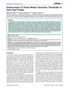
Figure 1: This figure shows the types of motion phenomena that involve temporal grouping. In each square, the top subfigure (labelled true) shows the data. The lower subfigure (labelled perceived) shows the perception given in psychophysical experiments. excitation, (iii) a columnar organization of visual features, and (iv) normalizing inhibition. Section (2) describes our theory. In section (3) we describe our computer simulations and how they compare with the data.

2

The Theory

Kalman filters [13] are a standard technique using prediction to improve state estimation over time. They have, for example, been successfully used to track the boundaries of hands in image sequences [4]. However, these filters need preprocessing, or data association [2], to determine which measurements in the

image should be used to update the hand model. More precisely, the boundary of the hand model should match edges extracted from the image. But a typical image contains many edges and so data association must be used to determine which edges correspond to the hand and should be used to update this model. Data association becomes very difficult for certain forms of tracking [4]. An alternative approach is based on a Bayesian model for prediction and estimation which includes standard Kalman filtering as a special case [10]. This approach has been successfully applied to hand tracking [12] and results in significantly improved performance. The key insight is that it performs data association (or temporal grouping) while doing prediction and estimation. In this approach, we let the state vector at time t be {~v(~x, t)}. The state vector represents the velocities at time t at every point ~x in the visual field. ~ x, t)} which represent We also have measurements {φ(~ the activities of motion sensitive observation cells responding to external stimuli. Again these are specified at every point in the visual field. We let Φ(t) = ~ x, t)}, {φ(~ ~ x, t − δ)}, ...) be the set of all measure({φ(~ ments up to, and including, time t. The model must estimate the state vector given the measurements. The Bayesian approach requires specifying: (i) a probability distribution, or likelihood function, Pl for the measurements conditioned on the external velocity, and (ii) a prior probability, or motion model, Pm for the motion field at t conditioned on the motion field at time t − δ. These are expressed as: ~ x, t)}|{~v(~x, t)}) and Pm ({~v (~x, t)}|{~v (~x, t − δ)}). Pl ({φ(~ (1) We let Pe ({~v (~x, t − δ)}|Φ(t − δ)) be the systems’ estimated probability distribution of the velocity field at time t − δ conditioned on all the previous measurements Φ(t − δ). To update Pe with time we use the prediction equation: Z Pp ({~v (~x, t)}|Φ(t − δ)) = d[~v (~x, t − δ)]

It can be shown [10] that if the measurement and prior probabilities (equation (1)) are both Gaussians, then equations (2,3) reduce to the standard Kalman equations which update the mean and the covariance of Pp and Pe over time. Gaussian distributions, however, are non-robust [11] and an incorrect (outlier) measurement can seriously distort the estimate of the true state, Therefore Gaussians are unable to solve the data association problem well. Instead we choose the measurement model Pl to be robust against outliers similar to the model used in [12], for details see next section, There is no requirement, however, that our motion model Pm be robust. Therefore we use a Gaussian model for prediction which assumes that the velocity is approximately constant between time frames with the covariance of the Gaussian determining what variations are allowed. For simplicity, we assume that the prior and the measurement distributions are chosen to be factorizable in spatial position, so that the probabilities at one spatial point are independent of those at another. In mathematical terms, this means that: Y Pm ({~v (~x, t)}|{~v(~x0 , t − δ)}) = pm (~v (~x, t)|{~v (~x0 , t − δ)}) ~ x

~ x, t)}|{~v (~x, t)}) = Pl ({φ(~

Y

~ x, t)|~v (~x, t)}). (4) pl (φ(~

~ x

These conditions imply that Pp and Pe can also be factorized as: Y Pp ({~v (~x, t)}|Φ(t − δ)) = pp (~v (~x, t)|Φ(t − δ)), ~ x

Pe ({~v (~x, t)}|Φ(t)) =

Y

pe (~v (~x, t)|Φ(t)), (5)

~ x

which means that we can update the estimates of ~v (~x, t) at each point ~x independently. It also means that we can normalize the velocities at each point inR dependently d~v (~x, t) = 1pe (~v (~x, t)|Φ(t)), ∀ ~x, t.

2.1

The motion model Pm

The motion model we use in this paper assumes that the velocities at different positions ~x are independent conditioned Q on the past velocities Pm ({~v (~x, t)}|{~v(~x0 , t − δ)}) = ~x pm (~v (~x, t)|{~v (~x0 , t − δ)}). Pm ({~v (~x, t)} |{~v (~x, t − δ)})Pe ({~v (~x, t − δ)}|Φ(t − δ)), (2) To proceed further, we discretize the set of allowed velocities and the set of spatial positions. The spatial and the estimation equation (derived from Bayes’ thepositions are set to be {~xi : i = 1, ..., N }. The velociorem): ties at ~xi are set equal to {~vµ : µ = 1, ..., M }. We then define ~ x, t)}|{~v(~x, t)})Pp ({~v (~x, t)}|Φ(t − δ)) the prediction model for discrete velocities: Pl ({φ(~ Pe ({~v (~x, t)}|Φ(t)) = , pm (~v (~x, t)|{~vµ (~xi , t − δ)}) ~ x, t)}|Φ(t − δ)) P ({φ(~ XX (3) = q(~v (~x, t); ~vµ(i) (~xi , t − δ), Σv , Σx ), (6) where the denominator is a normalizing term. µ i

~ x, t) takes all possible values such that Now φ(~ PN x, t) = 1 and φi (~x, t) ≥ 0, ∀i. By induci=1 φi (~ P ~ q(~v (~x, t); ~vµ (~xi , t − δ)) = G(~v (~x, t) − ~vµ (~xi , t − δ); Σv ) x, t) = (1/(N + 1)!)~1, where tion we prove that φ φ(~ G(~x − ~xi − δ~vµ (~xi , t − δ); Σx ) ~ , (7) 1 has components (1, 1, ..., 1). × K(~x, t) 2.3 The Algorithm where:

where G(., .) is a Gaussian and K(~x, t) is a normalization factor choosen to ensure that P (~v (~x, t)|{~vµ (~xi , t− δ)) is normalized. The covariances Σx and Σv are defined in a coordinate system based on the velocity vector ~vµ . They are diagonal in this cordinate system and are expressed in terms of their longitudinal and transverse components σx,l , σx,t , σv,l , σv,t . Typical values for these in our simulations are 1.0, 0.5, .2, 0.1 respectively.

2.2

The likelihood function Pl

At each point ~x in the image domain D and at each time t we have observations of these velocities. These are performed by a set of cells tuned to velocity vectors {~vi : i = 1, ..., M } These cells receive input from the image sequence. The observation activities {φi (~x, t)} of these observation cells are determined by a model such as [8] but for our simulations we use a simpler model described in [22]. The activities of P these cells are normalized (by an L1 norm) so that i φi (~x, t) = 1, ∀~x, t. The activities can therefore be interpreted as probabilities that the velocities ~vi are present at position ~x at time t. If no true velocities are present at, or in the neighborhood of, ~x then φi (~x, t) = 1/M and all velocities are considered to be equally likely at that point. Our likelihood function assumes that the observations of a cell are due to the true velocity at the centre of the cell and are independent spatially ~ x, t)|~v (~x, t)). ~ x, t)}|{~v(~x, t)}) = Q pl (φ(~ Pl ({φ(~ ~ x We set ~ x, t)|~vµ (~x, t)) = pl (φ(~

~ x, t) · f(~ ~ vµ (~x, t)) φ(~ . ~ vµ (~x, t)) · P φ(~ ~ x, t) f(~

(8)

φ

~ vµ (~x, t)) = (f1 (~vµ (~x, t)), ..., fM (~vµ (~x, t)) is where f(~ the tuning of the observation velocity cells µ to the interpretation velocity cells i. We set: e−(1/2)(~vi −~vµ )

fi (~vµ (~x, t)) = PM

j=1

T

Σ−1 (~ vi −~ vµ )

e−(1/2)(~vj −~vµ )

T Σ−1 (~ v

vµ ) j −~

, (9)

where Σ = Σv is the covariance matrix which depends of the direction of ~vµ (~x, t). It is specified in terms of its longitutinal and transverse components taking typP ical values 0.2, 0.1. Observe that M vµ (~x, t)) = i=1 fi (~ 1, ∀ µ, ~x, t.

Our algorithm proceeds by updating the velocity estimates using equations (2,3). As described in [22] this can be performed using a network model with properties similar to that of the visual cortex. This network model is parallelizable but, lacking a parallel computer, we simulated it on a Sun workstation.

3

The Experimental Results

We started by looking at the qualitative properties of the system for three motion phenomena. We first considered the improved accuracy of velocity estimation of a single dot over time [14]. Then we examined the predictions for the motion occlusion experiments [20]. Finally we investigated the motion outlier experiments [19],[9]. See [22] for details of how we simulated the input for these experiments.

3.1

Single Dot

Next we explored what would happen if the target dot entered an occluding region where no input measurements were made. The results, see figure (2), were the same as the previous case until the target dot reached the occluder. In the occluded region, the motion model continues to propagate the target dot but the probabilities start to diffuse and the estimate became less certain. This was demonstrated by comparing our results to those of the previous case and by plotting how the sharpness first increased with the number of frames and then started to fall off as the target entered the occluded region. Our figures also show how the estimation of the direction of velocity systematically started to degrade. These results showed that the model had still enough “momentum” to progate its estimate of the target dots position even though no measurements were available.

3.2

Single dot with occluders defined by distractor motion

We then tested our model with the occlusion experiments described in [20], see figures (3,4) We use the same measures and plots as for the single isolated dot. However, there are limitations to the sharpness and normalization measures if there are multiple motions per position as in the occlusion case. Thus we also plot the cells’ activities as a function of the velocity tuning, using 3D plots. For the case where the occluder is defined by motion perpendicular to the target motion, the plot indicates that the cella are maintaining probabilities for several motions at the same time. After

Figure 2: Single dot with occlusion. The right hand figure shows the result of the model after occlusion. Observe how the confidence and the sharpness both decrease rapidly but the dot is still propagated in the “correct” direction. The right hand figure shows that the sharpness decays as the target enters the occluder.

Figure 4: As the target dot enters the occluder tow peaks start developing in the probability distribution, frame 3. The bigger the occluder the more the peak induced by the motion of the distractor dots starts dominating, frames 5 and 6. But as the dot re-emerges form the occluder it rapidly becomes sharp again, frames 7 and 8.

3.3

Figure 3: The occuder is defined by vertical motion of distractor dots. The target motion, not shown, is horizontal from left to right.

entering the occluding region, the peak corresponding to the target motion gets smaller than the peak due to the occluders. However, the peak of the target remains and so the target peak can rapidly increase as the target exits from the occluders. The results are also consistent qualitatively with experiment for cases where the occluder contains motion parallel to the target’s motion. In these cases we find that the probabilities of velocity indeed get captured. In cases where the dot is perceived as being occluded, we observe two peaks in the probability distribution. One for the single dot and one for the distractors. If the distracting field is large then the single dot peak starts becoming very small.

Outlier Detection

In the outlier detection experiments [19], the target dot is undergoing regular motion but it is surrounded by distractor dots, which are undergoing random Brownian motion. Our first test of the model is when the target dot is moving straight. It can be seen that the target dot rapidly gets large sharpness and confidence by constrast to the distractor dots which are not moving coherently enough to gain confidence or sharpness. The sharpness does not grow monotonically because the distractor dots sometimes interfere with the target’s motion by causing distracting activity in the measurement cells. We also tested the model for circular outlier detection. In this case, again, the model suceeded in getting large sharpness and confidence for the target dot. Once again, the entropies and confidence were lower for this case than for the straight-line motion. This reflects the bias of the motion model. Similar biases may be found in the experimental data [19]. Our results of this problem are related to those obtained from the neural motivated model by Grzywacz et al. [9] who did detailed experimental tests of their model. This connection is being pursued in our cur-

Figure 5: Outlier Figure. A target dot starts at the extreme left and moves in a straightline from left to right. Our model successfully detcts it as the single coherent moving dot in the image.

Figure 7: Outlier figure for target dot moving with circular motion, The sharpness increases though with fluctuations cause by the distractor dots. The sharpness is less than for the straightline path in agreement with the psychophysical experiments. rent work.

4

Figure 6: The sharpness of the target dot quickly becomes high but it undergoes fluctuations as it interacts with the distractor dots.

Conclusion

This work provided a theory for temporal coherence. The theory was formulated in terms of Bayesian estimation using motion measurements and motion prediction. By incorporating robustness in the measurement model the system is able to do a form of temporal grouping (or data association) which enabled it to choose what data should be used to update the state estimation and what data could be ignored. The model seemed in qualitative agreement with a number of existing psychophyiscal experiments on motion estimation over time, motion occluders and motion outliers [15],[19],[20]. There is also interesting similarities between our network implementation and known properties of the visual cortex, see also [9]. These biological aspects of the work are being pursued elsewhere, see [22]. Finally, we emphasize that simple networks of the type we propose can implement Bayesian generalizations of Kalman filters. The popularity of standard linear Kalman filters is often due to pragmatic reasons of computational efficiency. Thus linear Kalman filters are often used even when they are inapproriate as models of the underlying processes. Though statistical sampling methods can be used successfully in some cases, see [12], high computational costs often limit the use of Bayesian techniques. We are therefore investigating the possibility of implementing our network in VLSI in the expectation that we will then be

able to do Bayesian estimation of motion in real time.

Acknowledgements We would like to thank the Office of Naval Research and ARPA for funding under grant number N0001495-1-1022. NMG was funded by the Air Force Grant AFOSR F49620-95-1-0265. Further support for this work came from core grant EY-06883 from the National Eye Institute to the Smith-Kettlewell Eye Research Institute.

References [1] S.M. Anstis and V.S. Ramachandran. “Visual inertia in apparent motion”. Vision Research 27, 755-764. 1987. [2] Bar-Shalom, Y., and Fortmann, T.E. Tracking and Data Association. Academic Press. 1988.

[12] M. Isard, M., and A. Blake “Contour tracking by stochastic propagation of conditional density”. Proc. European Conf. Comput. Vision, pp. 343356, Cambridge, UK. 1996. [13] R.E. Kalman. “A new approach to linear filtering and prediction problems.” Trans ASME J. of Basic Engineering. 1960. [14] S.P. McKee and L. Welch. “Sequential recruitment in the discrimination of velocity”. Journal of the Optical Society of America, A, 2, 243-251. 1985. [15] McKee, S.P., Silverman, G.H., and Nakayama, K. “Precise velocity discrimination despite random variations in temporal frequency and contrast”. Vision Res. 26, 609-619. 1986.

[3] M.J. Black and P. Anandan “Robust dynamic motion estimation over time”. Proc. Computer Vision and Pattern Recognition, CVPR-91. Maui, Hawaii. pp. 296-302. June 1991.

[16] K. Nakayama and G.H. Silverman. “Temporal and spatial characteristics of the upper displacement limit for motion in random dots”. Vision Research, 24, 293-299. 1984.

[4] Blake, A., Curwen, R., and Zisserman, A. “A framework for spatio-temporal control in the tracking of visual contours”. Int. J. Comput. Vision 11, 127-145. 1993.

[17] V.S. Ramachandran and S.M. Anstis. “Extrapolation of motion path in human visual perception”. Vision Research, 23, 83-85. 1983.

[5] Burr, D.C., Ross, J., and Morrone, M.C. “Seeing objects in motion”. Proc. Royal Soc. Lond. B 227, 249-265. 1986. [6] N.M. Grzywacz. Invest. Ophthalmol. Vis. vol. 28, p 300. 1987. [7] N.M. Grzywacz, J.A. Smith, and A.L. Yuille, “A computational framework for visual motion’s spatial and temporal coherence”. Proceedings IEEE Workshop on Visual Motion, Irvine. 1989. [8] N.M. Grzywacz and A.L. Yuille. “A model for the estimate of local image velocity by cells in the visual cortex”. Proceedings of the Royal Society of London. B. 239, pp 129-161. 1990. [9] Grzywacz, N.M., Watamaniuk, S.N.J., and McKee, S.P. “Temporal coherence theory for the detection and measurement of visual motion.” Vision Res. 35, 3183-3203. 1995. [10] Ho, Y-C. “A Bayesian approach to problems in stochastic estimation and control”. IEEE Trans. on Automatic Control 9, 333-339. 1964. [11] P.J. Huber. Robust Statistics. John Wiley and Sons. New york. 1981.

[18] S.N.J. Watamaniuk. “Visible persistence is reduced by fixed-trajectory motion but not by random motion.” Perception, 21, 791-802. 1992. [19] S.N.J. Watamaniuk, S.P. McKee, and N.M. Grzywacz. “Detecting a Trajectory Embedded in Random-Direction Motion Noise.” Vision Research. 35, 65-77. 1994. [20] Watamaniuk, S.N.J., and McKee, S.P. “Seeing motion behind occluders”. Nature 377, 729-730. 1995. [21] A.L. Yuille and N.M. Grzywacz. “A Theoretical Framework for visual Motion”. To appear in High-level motion processinginterdisciplinary approach-.. Eds. T. Watanabe. North Holland Press. 1996. [22] A.L. Yuille, P-Y Burgi, and N.M Grzywacz. “Visual Motion Estimation and Prediction”. SmithKettlewell Eye Research Institute Preprint. 1997.