383
J. Service Science & Management, 2010, 3, 383-389 doi: 10.4236/jssm.2010.34045 Published Online December 2010 (http://www.SciRP.org/journal/jssm)
Volatility Forecasting of Market Demand as Aids for Planning Manufacturing Activities Jean-Pierre Briffaut1,3, Patrick Lallement2,3 1
Institut Telecom-Telecom & Management SudParis, Evry, France; 2Université de Technologie de Troyes (UTT), Troyes, France; Charles Delaunay Institute, Troyes, France. Email:
[email protected]
3
Received August 20th, 2010; revised October 12th, 2010; accepted November 11th, 2010.
ABSTRACT The concepts and techniques designed and used for pricing financial options have been applied to assist in scheduling manufacturing activities. Releasing a manufacturing order is viewed as an investment opportunity whose properties are similar to a call option. Its value can be considered as the derivative of the market demand mirrored in the selling price of the manufactured products and changes over time following an Itô process. Dynamic programming has been used to derive the optimal timing for releasing manufacturing orders. It appears advisable to release a manufacturing when the unit selling price come to a threshold P* given by the relation P* = β/(β – 1) C with C = unit cost price. β is a parameter whose value depends on the trend parameter α and the volatility σ of the selling price, the discount rate ρ applicable to the capital appreciation relevant to the business context under consideration. The results have been successfully applied to the evolution of the quarterly construction cost index in France over ten years. Keywords: Forecasting, Uncertainty, Stochastic process, Dynamic Programming, Manufacturing Activities
1. Introduction Since the dawn of entrepreneurship men have been calculating the chances of success in future actions by assessing the available statistics, if any, on past actions. But entrepreneurs1 are confronted with their interpretation in terms of what is actually measured and how they are reliable. A wide range of mathematical strands has been developed to deal with the ongoing uncertainty of the economic environment in the field of financial economicsoptions, futures, other derivatives - as well as capital budgeting [1]. In this paper we aim to demonstrate how the concepts and techniques used in these fields can contribute to scheduling manufacturing activities. Scheduling the manufacturing of a batch of products is considered as an option analogous to a financial call option on a common stock market. When deciding on a schedule, the option to manufacture is “killed” giving up the possibility of waiting for complementary information about the market. The objectives of this paper are threefold: 1) to produce the understanding and definitions of 1
Entrepreneur: one who undertakes a business or enterprise with chance of profit or loss (Oxford Dictionary)
Copyright © 2010 SciRes.
several concepts associated with the way uncertainty is dealt with in financial economics; 2) to demonstrate how this mindset can be used to engineer the schedule of manufacturing activities in volatile contexts; 3) to show how the technique explained can be applied on the basis of an example. In Section 2 is explained the way the timing of a decision impacts its relevance in a perspective of manufacturing activities. Section 3 describes the mathematical background pertaining to the application of stochastic processes to deal with risk. Section 4 focuses on the paradigm of uncertainty engineered to cancel the risk in the domain of financial options and its practical use for manufacturing project. In Section 5 an example is presented on the basis of data relating to the construction cost index in France. Section 6 touches on the main assumptions underlying the Itô process and on the relevance of the option pricing model for forecasting purposes.
2. Forecasting and the Option Approach in a Perspective of Manufacturing Activities How should a manufacturing company, facing uncerJSSM
384
Volatility Forecasting of Market Demand as Aids for Planning Manufacturing Activities
tainty over future market conditions, decide on its production schedule? To keep on top of demand, a company has to avoid shortages on one hand and too much inventtory on the other. This means that forecasting is a key issue, whether the company builds its own products in its own factories or outsources its production. Short of being able to control market, demand planning and scheduling manufacturing operations depend on an ability to predict what will be the market demand and how it will fluctuate during the execution of plans generally frozen over a certain horizon. Forecasting by extrapolating historical data (linear regression, simple and double exponential smoothing, decomposition of time-series in trends, cyclical variations and randomness …..) [2] is a technique over-described in textbooks and research papers. It is straightforward to apply and could be justified in the postwar “fordist” era. Today volatility is the key feature of the global economy: the fluttering of a butterfly in Bejing can trigger a tornado in Cuba. The irreversibility of a decision and the possibility of delaying its implementation are two important characteristics when converting forecasts into scheduled courses of action. A manufacturing company with an opportunity to schedule production is holding an “option” analogous to a financial call option on a common stock - it has the right and not the obligation, at some future time of its choosing, to make an expenditure (manufacturing a batch of products) and receive a revenue (the proceeds of their sale) [3]. When such a company decides on a schedule, it exercises, or “kills”, its option to manufacture. It gives up the possibility of waiting for complementary information to arrive that might affect the desirability or timing of the expenditure incurred by the scheduled production versus the market value of the manufactured products, value which fluctuates stochastically. The option can be “in the money” meaning that when it is exercised it would yield a positive payoff. It is said to be “out of the money” if exercising yields a negative payoff. It cannot disinvest2 that is get back the money already spent, should market conditions change adversely. An investment project, such as manufacturing a batch of products, can be made more valuable if it gives the manufacturer the option to expand when economic conditions become favorable. That option to expand in the future clearly has a value. The higher the volatility of the underlying asset - the market demand - the higher value is given to the option - the market value of the batch of products manufactured to sell. Economists assume that the selling price of a product depends on the market demand expressed in terms of quantity of products so that the proceeds of a sale increase along with market deCopyright © 2010 SciRes.
mand.
3. Market Volatility and the Associated Risks 3.1. Volatility Volatility is the relative rate at which market demand moves up and down. It is found by calculating, over a period of time, the standard deviation of daily, weekly or monthly change in market demand. The time intervals considered are impelled to be chosen by the behavior of market demand. If it moves up and down rapidly over short periods of time, it is highly volatile. On the contrary if market demand is almost never changed it has low volatility. The risk that the scheduler of manufacturing activities is exposed to, is based on the potential for the volatility of the underlying market demand or the market’s perception of that volatility to change. It is generally assumed that uncertainty in the future depends on the time span. The longer the time interval, the greater is uncertainty about the situation by the end of this time interval and, as a consequence, the volatility of a variable z under consideration. To match with this commonly accepted belief, the time-dependent probability density function of the variable z at a fixed time, when normally distributed, is [4] f z, t
z2 exp 2 .t 2t 1
(1)
The mean value of z at any time t is E z , t 0 and the variance of z at time t is Var z , t t . In many contexts of business life changes in the values of a variable are not measured in absolute terms but as increments with respect to its values, that is in relative terms. That is why volatility is calculated as the variance of a log function representing the values of a variable at different times. Denoting the market demand as D i for the time interval i , the volatility of this variable is defined as the standard deviation of the function ln D i / Di 1 with 1 i n .
3.2. Wiener Process A Markov process is a particular type of stochastic process where only the present value of a variable is relevant for predicting the future. The past history of the variable is supposed to be embedded in its present value. Predictions for the future are uncertain and must be expressed in terms of probability distribution. If the weak form of market efficiency were not true, analysts could make above-average returns on stocks by interpreting the charts of the past history. JSSM
Volatility Forecasting of Market Demand as Aids for Planning Manufacturing Activities
The variable z following a Wiener process has a mean change of zero and a variance rate of 1 per time unit. The Wiener process has been used in physics to describe what is referred to as geometric Brownian motion [5]. The change z during a period of time t is z t
(2)
where has a standard normal distribution N(0,1). The values of z for any two different t are statistically independent. If a finite time interval T is broken down into N time intervals t so that N t , t T , the difference z T z 0 is described by the sum of statistically independent increments n
i .
t
(3)
i 1
The volatility of z over the time span T is the variance of z T z 0 , that is T . When the market demand D is assumed to follow the rules of the geometric brownian motion, it evolves according the equation dD Ddt Ddz
(4)
where dz is the increment of a Wiener process. A variable evolving in this way is said to follow an Itô process. This is precisely the model chosen by [6] for the contingent claims analysis of options. Equation (4) implies that the current value of D is known, but future values are log-normally distributed with a variance that grows linearly with the time horizon. Thus although information arrives over time ( D is changing) the future market value of the production remains uncertain. Equation (4) describes the percentage changes in D , dD / D , which are the changes in the natural logarithm of D .
3.3. Itô’s Lemma Suppose that a variable x follows an Itô process such that dx x, t xdt x, t xdz
(5)
Itô’s lemma [7] shows that the differential of a function G x, t is characterized by (4), it will be necessary to compute variations dV . We can expand variations dV by using the Itô’s lemma which leads to G G 1 2 G 2 2 G x x dt xdz dG 2 x x t 2 x
(6)
4. Uncertainty and the Analogy to Financial Options 4.1. General Considerations 2
To disinvest: to realize invested assets of a person, institution… (Oxford Dictionary)
Copyright © 2010 SciRes.
385
It is generally accepted that there is an immediate correspondence between selling price and market demand. In fact the selling price of manufactured products increases along with the market demand when a specified constant quantity of products is made available in the market place. If the unit cost price is higher than the unit selling price the payoff is negative. If the unit cost price is lower than the unit selling price, then the payoff turns positive. Demand volatility describes the randomness of market behaviour and selling price. Therefore the selling price P and, as a consequence, the value of a manufacturing batch are determined by the market demand D in terms of the quantity of products asked by customers. Two types of reasoning can be envisaged when scheduling manufacturing activities. The first one is developed by insurers. The selling price is forecast for future time periods with an expected value (mean) and a standard deviation that is regarded as the measure of the risk incurred. The quantity of products to manufacture is adjusted to the expected selling prices. When the manufactured products become available in the market place with some manufacturing lead times, the market prices turn higher or lower than the cost prices. In this situation the attitude of the forecaster is to consider that over a large number of time periods the cumulative payoffs turn positive. A second type of reasoning is followed by traders. Their strategy is to follow the market dynamics not to minimize risks but to cancel them for each course of action. This is engineered by a hedging mechanism. Within a manufacturing context the tactics taken by a scheduler can be to choose the timing to release manufacturing orders and the quantity to manufacture intended to satisfy a specified proportion of customers. In this paper we assume that deciding on releasing a manufacturing order depends only on the unit selling price P and the unit cost price C . Let us see how this technique can be applied to scheduling manufacturing activities. The opportunity value of the option to release a manufacturing order today depends on a stochastic process for P . The problem is to find the future value V of the option today. To solve this problem, two approaches can be called on, i.e. the technique of portfolio and dynamic programming [8,9]. Both of them yield the same result [10]. In our case the solution by dynamic programming is more straightforward and is chosen.
4.2. Pricing a Manufacturing Option V(t) The value V t is a growing function of the selling price P. The selling price P t is supposed to follow a Wiener process as (4) and then its derivative writes JSSM
386
Volatility Forecasting of Market Demand as Aids for Planning Manufacturing Activities
dP Pdt Pdz
(7)
In the first step let us consider the deterministic evolution of P , i.e. = 0. The value of the manufacturing opportunity at time T is V P, T P (0).e T C .e T
(11)
(12)
Hence, using (11,12), it leads to
P
V 1 2 2 2V V P P 2 P 2
(13)
Equation (13) as to be solved with the boundary conditions V 0 0
V P * P * C V / P 1 when P P * Copyright © 2010 SciRes.
1 1 2 2 2 2 1 2 2
P*
(10)
Expanding dV using Itô’s lemma (6) gives V 1 2 2 2V P E dV P dt P 2 P 2
2
(18)
From the other boundary conditions (15,16) it is deduced that
That means it is advisable to launch the manufacturing of products when the selling price goes beyond C / . Then, P 0 is considered as the optimal price P* to release a manufacturing order. In the second step we have to consider the situation for σ ≠ 0. To calculate the value of the option two situations are taken into account. After the manufacturing order has been released the value of the option equals the unit selling price minus the unit cost price incurred C , i.e. V P P C . Before the manufacturing order has not been released the manufacturing opportunity yields a return from its capital appreciation at the discount rate . When applying the Itô’s lemma (6) it appears that V t , the derivative of the underlying selling price P , is also governed by a Wiener process (4). The expected value of dV induced by P t during the time interval dt writes E dV Vdt
(17)
Two roots are found. The negative one does not fulfil the boundary condition (14) so that the other one whose value is higher than 1 is left. The valid value solution for is given by
(9)
It leads to T * =0 when C / P 0 =1 or P 0 C / C
2 1 / 2 0
(8)
with , otherwise V P, T would increase indefinitely without delivering an optimal value for T . is the discount rate. Differentiating V P, T with respect to T yields the value T * maximizing V P, T T * 1/ ln C / P 0
(16) expresses the continuity condition at the junction point P P * with V P P C ). The solution of the differential equation (13) is V P A.P such that P is a root of the quadratic equation
(14) (15) (16)
C 1
(19)
and A
P * C
P *
(20)
It turns out that the solutions are V P * C P / P * when P P * and V P C when P P * (21) It can be shown that / 1 increases as inwe have 1 and creases. As / 1 . In other words, ceteris paribus, the higher the uncertainty about the market price measured by , the higher is the selling P * required to release a manufacturing order. This conclusion is fully in line with what the intuitive common sense expects.
4.3. Concluding Remarks In this section, we have shown that the optimal selling price P * to release a manufacturing order in a deterministic situation contrasts strongly with this that is valid in a stochastic situation characterized by its volatility . We think that this result can assist efficiently in scheduling manufacturing activities because the number of parameters required is limited and can be easily deduced from past observation on the supposition that the future behaviour of the market demand can be deduced from the past.
5. Example of Application 5.1. Variations in the Construction Cost Index Derived from Observations in the Construction Sector The quarterly variations in the French construction cost index over 10 years (1999-2008) are presented Table 1. JSSM
387
Volatility Forecasting of Market Demand as Aids for Planning Manufacturing Activities
These figures reflect the market price for products and services linked with this economic sector. In one way or the other the values of materials and services provided in this economic sector are strongly correlated to this construction cost index. Launching a development project in the construction sector depends heavily on the economic context. When the economy is sluggish, the investor-readiness to start a project is restrained. On the contrary, when the economic conditions are favorable, investors are inclined towards undertaking capital-intensive projects such as developing building sites. Their attitude is similar to that of option traders. On the other hand the construction sector monitors the activities of many upstream manufacturing industries (metallurgical, electrical, mechanical…). This is why the construction index was chosen as a relevant point of reference. Figure 1 gives the scatter diagram of indexes X and time intervals in an attempt to gain an impression of the relation between the construction cost indexes and time intervals. It shows a positive correlation. As the Itô process refers to a deterministic exponential function combined with “noisy” variations constituting the stochastic part of the index variations we tried to fit the set of data by an exponential regression. The form of the exponential curve is X t
(22)
where γ and δ are parameters to be estimated from the data. Denoting these estimates by c and d respecttively, we can estimate X by X from the data regression curve X c.d t (23) Taking natural logarithms we obtain the regression curve Table 1. Quarterly variations in the construction cost index in France from 1999 till 2008 (source: INSEE). Year
1st Q
2nd Q
3rd Q
4th Q
1999
1071
1074
1080
1065
2000
1083
1089
1093
1127
2001
1125
1139
1145
1140
2002
1159
1163
1170
1172
2003
1183
1202
1203
1214
2004
1225
1267
1272
1269
2005
1270
1276
1278
1332
2006
1362
1366
1381
1406
2007
1385
1435
1443
1474
2008
1497
1562
Copyright © 2010 SciRes.
Figure 1. Scatter diagram of construction cost indexes over time (derived from Table 1).
ln Xˆ ln c ln d t
Each pair of observations tion
X i , ti
(24) satisfies the rela-
ln X i ln c ln d ti ei a b ti ei
(25)
where ei is a stochastic variation at time ti . The least-squares fitting procedure gives X = 1036* (1.0095) t = 1036* exp t where = ln (1,0095) = 0,00945516 A measure of the quality of fit is given by the correlation coefficient RE square which is here 0,967. The standard deviation of ei gives the parameter , and we obtain = 0,016. The relative variations per quarter in X / X are plotted Figure 2 showing the spreads of i for each quarter with respect to . X / X for time interval i writes when t = 1(quarter):
X / X i i 5.2. Uses of the Previous Results The forecasted values of X for quarters after the 2nd quarter of 2008 valued 1562 are given by: X (t) = 1562*(1.0095) t
where t is measured in quarters starting in the 3rd quarter 2008. Since the standard deviation of changes in X grows with the square root of the time horizon, the upper and lower bounds of a 68-percent forecast confidence interval (Gaussian distribution) write respectively plus and minus 1562*(1.0095) t (1.0255)√t . The optimal value of X is derived from the equation / 1 C . The only unknown in the expression of
JSSM
388
Volatility Forecasting of Market Demand as Aids for Planning Manufacturing Activities
business. The constraint means that manufacturing a batch of products is worthwhile when the anticipated yield is higher than the increase rate of the market demand in terms of selling price. Evaluating for a company is quite an exercise and a lot of discussion has taken place to devise practical approaches. Calculating a relevant cost price is also another difficult issue: the advent of what is called ABC (Activity-Based Costing) proves the shortcomings of traditional methods.
6. Conclusions Figure 2. Scattergraph of dX/X around . 20 18 16
Beta/(Beta-1)
14 12 10 8 6 4 2 0 0,01
0,015
0,02
0,025
0,03
0,035
0,04
0,045
0,05
0,055
0,06
discount rate
Figure 3. / 1 versus .
is the discount rate per quarter . Figure 3 portrays the variations in / 1 as a function of . and are given the values derived from the exponential regression we carried out.
5.3. Application to Scheduling Manufacturing Activities The application of the model we presented requires the availability of a very limited number of parameters. As a consequence it should be easily used by scheduling departments of manufacturing companies. On one hand two of them reflect the market’s behaviour, i.e. its evolution given by α characterizing its exponential change over time and σ its volatility. They can be easily derived from historical market data that is generally easily accessible. On the other hand the discount rate and the unit cost price C have to be derived from managerial data. They are easier to describe than to determine. We have seen that the discount rate ρ must be higher than the trend parameter of the selling price. Otherwise the manufacturing project would never be profitable. This constraint makes sense economically speaking. In fact the discount rate is definitely not the ruling market interest rate but the current or targeted return on investment (ROI) available on the operations run by a Copyright © 2010 SciRes.
It is important to bear in mind that the Itô process we presented and used in this paper rests on many assumptions of which the main ones are mentioned hereafter. The first one refers to the type of randomness we dealt with. The validity of the Itô process we worked with depends entirely on whether market demand and selling prices really do fit the Gaussian curve. That means that uncertainty is proportional to t1/2. Thus in other words it is assumed that the deviation of market demand and correlated selling prices is directly proportional to the square root of time. This is strongly challenged by Mandelbrot and his followers [11,12] in many circumstances. The bell-shaped Gaussian curve reflects a form of chance called “mild” by Mandelbrot because it does not account for extreme events. The second assumption we have to consider is the current relevance of what is called a Markov process. It is supposed that the increments z for any two different time intervals t are statistically independent, which proves wrong in many situations because longterm correlations exist [11]. In addition to these restrictive conditions that command the validity of the option pricing model, another question can be raised: is the option pricing model more suitable than other models to produce relevant conclusions? The model described here is based on the analysis of historical series, like other standard forecasting techniques (exponential smoothing, Bass and Gompertz differential equations, Fourier series…). In business practice, several forecasting models are used concurrently for two main reasons: 1) achieving the adjustment of model parameters does not prove that the model is valid: least-square methods do well; 2) arguments advanced to decide which forecasting model is best are difficult to be put forward. Furthermore what was valid in the past does not preclude that the future may behave according another model. The option pricing model is eligible for forecasting economic activities such as manufacturing along with other standard models when the decision-making context is comparable with that found for financial option tradJSSM
Volatility Forecasting of Market Demand as Aids for Planning Manufacturing Activities
389
Corporate Liabilities,” Journal of Political Economy, Vol. 81, No. 3, May - June 1973.
ing.
REFERENCES
[7]
K. Itô, “On Stochastic Differential Equations,” Memoirs American Mathematical Society, 1951.
[1]
R. Elliott and E. Kopp, “Mathematics of Financial Markets,” Springer Finance, 2004.
[8]
[2]
S. Thomassey, “Méthodologies de la Prévision des Ventes Appliquée à la Distribution Textile,” (In French) Thèse D’automatique et Informatique Industrielle, Lille 1, 2002.
R. E. Bellman, “Dynamic Programming,” Princeton Unversity Press, New Jersy, 1957, Dover Paperback Edition 2003.
[9]
A. K. Dixit, “Optimization in Economic Theory (Chapter 11),” Oxford University Press, 1990.
[3]
J. C. Hull, “Options, Futures and Other Derivatives,” (Chapter 12), Prentice Hall, 2005.
[4]
T. L. Saaty and J. M. Alexander, “Thinking with Models (Chapter 3) ,” Pergamon Press, Oxford, England, 1981.
[5]
P. Lévy, “Processus Stochastiques et Mouvement Brownien,” 2ème Edition, Gauthier Villard, Paris, 1965.
[6]
F. Black and M. Scholes, “The Pricing of Options and
Copyright © 2010 SciRes.
[10] A. K. Dixit and R. S. Pindyck, “Investment under Uncertainty (Chapter 5),” Princeton University Press, New Jersy, 1994. [11] B. B. Mandelbrot and R. L. Hudson, “The (mis) Behaviours of Markets (Chapter 2),” Profile Books Ltd., London, 2004. [12] J. Lévy Véhel et Chr. Walter, “Les Marchés Fractals (In French), ” PUF 2002.
JSSM