Upcoming
Conferences
URISA’s 46th Annual Conference & Exposition
w w w. u r i s a . o r g
October 7–10, 2008 — New Orleans, LA
URISA Leadership Academy
December 8–12, 2008 — Seattle, WA
13th Annual GIS/CAMA Technologies Conference
February 8–11, 2009 — Charleston, SC
URISA’s Second GIS in Public Health Conference June 5–8, 2009 — Providence, RI
URISA/NENA Addressing Conference TBD
URISA’s 47th Annual Conference & Exposition
September 29–October 2, 2009 — Anaheim, CA
GIS in Transit Conference
November 11–13, 2009 — St Petersburg, FL
Volume 20 • No. 1 • 2008 Journal of the Urban and Regional Information Systems Association
Contents Refereed 5
Automatic Generation of High-Quality Three-Dimensional Urban Buildings from Aerial Images Ahmed F. Elaksher and James S. Bethel
15
Robust Principal Component Analysis and Geographically Weighted Regression: Urbanization in the Twin Cities Metropolitan Area of Minnesota Debarchana Ghosh and Steven M. Manson
27
Where Are They? A Spatial Inquiry of Sex Offenders in Brazos County Praveen Maghelal, Miriam Olivares, Douglas Wunneburger, and Gustavo Roman
35
Tools And Methods For A Transportation Household Survey Martin Trépanier, Robert Chapleau, and Catherine Morency
45
Mapping Land-Use/Land-Cover Change in the Olomouc Region, Czech Republic Tomáš Václavík
Plus 53
Mapping the Future Success of Public Education
Journal Publisher:
Urban and Regional Information Systems Association
Editor-in-Chief:
Jochen Albrecht
Journal Coordinator:
Scott A. Grams
Electronic Journal:
http://www.urisa.org/journal.htm
EDITORIAL OFFICE: Urban and Regional Information Systems Association, 1460 Renaissance Drive, Suite 305, Park Ridge, Illinois 60068-1348; Voice (847) 824-6300; Fax (847) 824-6363; E-mail
[email protected]. SUBMISSIONS: This publication accepts from authors an exclusive right of first publication to their article plus an accompanying grant of nonexclusive full rights. The publisher requires that full credit for first publication in the URISA Journal is provided in any subsequent electronic or print publications. For more information, the “Manuscript Submission Guidelines for Refereed Articles” is available on our website, www.urisa. org, or by calling (847) 824-6300. SUBSCRIPTION AND ADVERTISING: All correspondence about advertising, subscriptions, and URISA memberships should be directed to: Urban and Regional Information Systems Association, 1460 Renaissance Dr., Suite 305, Park Ridge, Illinois, 60068-1348; Voice (847) 824-6300; Fax (847) 824-6363; E-mail
[email protected]. URISA Journal is published two times a year by the Urban and Regional Information Systems Association. © 2008 by the Urban and Regional Information Systems Association. Authorization to photocopy items for internal or personal use, or the internal or personal use of specific clients, is granted by permission of the Urban and Regional Information Systems Association. Educational programs planned and presented by URISA provide attendees with relevant and rewarding continuing education experience. However, neither the content (whether written or oral) of any course, seminar, or other presentation, nor the use of a specific product in conjunction therewith, nor the exhibition of any materials by any party coincident with the educational event, should be construed as indicating endorsement or approval of the views presented, the products used, or the materials exhibited by URISA, or by its committees, Special Interest Groups, Chapters, or other commissions. SUBSCRIPTION RATE: One year: $295 business, libraries, government agencies, and public institutions. Individuals interested in subscriptions should contact URISA for membership information. US ISSN 1045-8077
2
URISA Journal • Vol. 20, No. 1 • 2008
Editors and Review Board URISA Journal Editor
Article Review Board
Editor-in-Chief
Peggy Agouris, Department of Spatial Information Science and Engineering, University of Maine
Jochen Albrecht, Department of Geography, Hunter College City University of New York
Thematic Editors Editor-Urban and Regional Information Science
Vacant Editor-Applications Research
Lyna Wiggins, Department of Planning, Rutgers University Editor-Social, Organizational, Legal, and Economic Sciences
Ian Masser, Department of Urban Planning and Management, ITC (Netherlands) Editor-Geographic Information Science
Mark Harrower, Department of Geography, University of Wisconsin Madison Editor-Information and Media Sciences
Michael Shiffer, Department of Planning, Massachusetts Institute of Technology Editor-Spatial Data Acquisition and Integration
Gary Hunter, Department of Geomatics, University of Melbourne (Australia) Editor-Geography, Cartography, and Cognitive Science
Vacant Editor-Education
Karen Kemp, Director, International Masters Program in GIS, University of Redlands
Section Editors Software Review Editor
Jay Lee, Department of Geography, Kent State University Book Review Editor
David Tulloch, Department of Landscape Architecture, Rutgers University
URISA Journal • Vol. 20, No. 1 • 2008
Grenville Barnes, Geomatics Program, University of Florida Michael Batty, Centre for Advanced Spatial Analysis, University College London (United Kingdom) Kate Beard, Department of Spatial Information Science and Engineering, University of Maine Yvan Bédard, Centre for Research in Geomatics, Laval University (Canada) Barbara P. Buttenfield, Department of Geography, University of Colorado Keith C. Clarke, Department of Geography, University of California-Santa Barbara
Kingsley E. Haynes, Public Policy and Geography, George Mason University Eric J. Heikkila, School of Policy, Planning, and Development, University of Southern California Stephen C. Hirtle, Department of Information Science and Telecommunications, University of Pittsburgh Gary Jeffress, Department of Geographical Information Science, Texas A&M UniversityCorpus Christi Richard E. Klosterman, Department of Geography and Planning, University of Akron Robert Laurini, Claude Bernard University of Lyon (France) Thomas M. Lillesand, Environmental Remote Sensing Center, University of WisconsinMadison Paul Longley, Centre for Advanced Spatial Analysis, University College, London (United Kingdom)
David Coleman, Department of Geodesy and Geomatics Engineering, University of New Brunswick (Canada)
Xavier R. Lopez, Oracle Corporation
David J. Cowen, Department of Geography, University of South Carolina
Harvey J. Miller, Department of Geography, University of Utah
David Maguire, Environmental Systems Research Institute
Massimo Craglia, Department of Town & Regional Planning, University of Sheffield (United Kingdom)
Zorica Nedovic-Budic, Department of Urban and Regional Planning,University of IllinoisChampaign/Urbana
William J. Craig, Center for Urban and Regional Affairs, University of Minnesota
Atsuyuki Okabe, Department of Urban Engineering, University of Tokyo (Japan)
Robert G. Cromley, Department of Geography, University of Connecticut
Harlan Onsrud, Spatial Information Science and Engineering, University of Maine
Kenneth J. Dueker, Urban Studies and Planning, Portland State University
Jeffrey K. Pinto, School of Business, Penn State Erie
Geoffrey Dutton, Spatial Effects
Gerard Rushton, Department of Geography, University of Iowa
Max J. Egenhofer, Department of Spatial Information Science and Engineering, University of Maine
Jie Shan, School of Civil Engineering, Purdue University
Manfred Ehlers, Research Center for Geoinformatics and Remote Sensing, University of Osnabrueck (Germany)
Bruce D. Spear, Federal Highway Administration
Manfred M. Fischer, Economics, Geography & Geoinformatics, Vienna University of Economics and Business Administration (Austria) Myke Gluck, Department of Math and Computer Science, Virginia Military Institute Michael Goodchild, Department of Geography, University of California-Santa Barbara
Jonathan Sperling, Policy Development & Research, U.S. Department of Housing and Urban Development David J. Unwin, School of Geography, Birkbeck College, London (United Kingdom) Stephen J. Ventura, Department of Environmental Studies and Soil Science, University of Wisconsin-Madison Nancy von Meyer, Fairview Industries
Michael Gould, Department of Information Systems Universitat Jaume I (Spain)
Barry Wellar, Department of Geography, University of Ottawa (Canada)
Daniel A. Griffith, Department of Geography, Syracuse University
Michael F. Worboys, Department of Computer Science, Keele University (United Kingdom)
Francis J. Harvey, Department of Geography, University of Minnesota
F. Benjamin Zhan, Department of Geography, Texas State University-San Marcos
3
Automatic Generation of High-Quality Three-Dimensional Urban Buildings from Aerial Images Ahmed F. Elaksher and James S. Bethel Abstract: High-quality three-dimensional building databases are essential inputs for urban area geographic information systems. Because manual generation of these databases is extremely costly and time-consuming, the development of automated algorithms is greatly needed. This article presents a new algorithm to automatically extract accurate and reliable three-dimensional building information. High overlapping aerial images are used as input to the algorithm. Radiometric and geometric properties of buildings are utilized to distinguish building roof regions in the images. This is accomplished with image segmentation and neural network techniques. A rule-based system is employed to extract the vertices of the roof polygons in all images. Photogrammetric mathematical models are used to generate the roof topology and compute the three-dimensional coordinates of the roof vertices. The algorithm is tested on 30 buildings in a complex urban scene. Results showed that 95 percent of the building roofs are extracted correctly. The root-mean-square error for the extracted building vertices is 0.35 meter using 1:4000 scale aerial photographs scanned at 30 microns.
Introduction Three-dimension building information is required for a variety of applications, such as urban planning, mobile communication, visual simulation, visualization, and cartography. Automatic generation of this information is one of the most challenging problems in photogrammetry, image understanding, computer vision, and GIS communities. Current automated algorithms have shown some progress in this area. However, some deficiencies still remain in these algorithms. This is particularly apparent in comparison to manual extraction techniques, which, although slow, are essentially perfect in accuracy and completeness. Recent research covers extracting building information from high-resolution satellite imageries, high-quality digital elevation models (DEMs), and aerial images. For example, QuickBird and IKONOS high-resolution satellite imageries are used to acquire planemetric building information with one-meter horizontal accuracy (Theng 2006, Lee et al. 2003). However, aerial images are the primary source used to acquire accurate and reliable geospatial information. Lin and Nevatia (1998) proposed an algorithm to extract building wireframes from a single image. However, a single image does not provide any depth information. A pair of stereo images could also be used to extract building information (Avrahami et al. 2004, Chein and Hsu 2000). Using one pair of images is insufficient to extract the entire building because of hidden features that are not projected into the image pair. Kim et al. (2001) presented a model-based approach to generate buildings from multiple images. Three-dimensional rooftop hypotheses are generated using three-dimensional roof boundaries and corners extracted from multiple images. The generated hypotheses then are employed to extract buildings using an expandable Bayesian network. Wang and Tseng (2004) proposed a semiautomatic approach to extract buildings from multiple views. They proposed an abstract floating model to represent real URISA Journal • Elaksher, Bethel
objects. Each model has several pose and shape parameters. The parameters are estimated by fitting the model to the images using least-squares adjustment. The algorithm is limited to parametric models only. In Shmid and Zisserman (2000), lines are extracted in the images and matched over multiple views in a pair-wise mode. Each line then is assigned two planes, one plane on each side. The planes are rotated, and the best-fitting plane is found. Planes then are intersected to find the intersection lines. Henricsson et al. (1996) presented another system to extract suburban roofs from aerial images by combining two-dimensional edge information together with photometric and chromatic attributes. Edges are extracted in the images and aggregated to form coherent contour line segments. Photometric and chromatic contour attributes for adjacent regions around each contour are assigned to it. For each contour, attributes are computed-based on the luminance, color, proximity, and orientation, and saved for the next step. Contour segments then are matched using their attributes. Segments in three dimension are grouped and merged according to an initial set of plane hypotheses. Fischer et al. (1997) extracted three-dimensional buildings from aerial images using a generic modeling approach that depends on combining building parts. The process starts by extracting low-level image features: points, lines, regions, and their mutual relations. These features are used to generate three-dimensinal building part hypotheses in a bottom-up process. A step-wise model-driven aggregation process combines the three-dimensional building feature aggregates to three-dimensional parameterized building parts and then to a more complex building descriptor. The resulting complex three-dimensional building hypothesis then is back-projected to the images to allow component-based hypothesis verification. A semiautomated approach is used in Förstner (1999) to solve the building-extraction problem. First, the user has to define the building model and find the building elements in one image 5
by a number of mouse clicks. Then the algorithm finds the corresponding features in other images and matches them to build the three-dimensional wireframe of the building. This approach supports the extraction of more complex buildings; however, it requires the user to spend a great amount of time interacting with the system. Rottensteiner (2000) presented a semiautomated building-extraction technique in which the user can select an appropriate building primitive from a database and then adjust the parameters of the primitive to the actual data by interactively measuring points in the digital images, and determine the final building parameters by automated matching tools. High-quality DEMs such as those available from light detection and ranging (LIDAR) have been used to generate three-dimensional building models. Tse et al. (2006) proposed an algorithm based on segmenting the raw data into high and low regions, and then modeling the walls and roofs by extruding the triangulated terrain surface (TIN) using CAD-type Euler operators. Tarsha-Kurdi et al. (2006) proposed another algorithm that discriminates terrain and off-terrain clouds in a LIDAR point cloud. Then it categorizes the off-terrain points to building and vegetation subclasses. Building points then are detected via segmenting the original LIDAR three-dimensional point cloud. In Brunn and Weidner (1997), the digital surface models (DSMs) are extracted using mathematical morphology. The differences between the DEMs and the DSMs are computed and building points are detected by thresholding these differences. In the next step, building wireframes are generated using parametric and prismatic models depending on the complexity of the detected building. Morgan and Habib (2002) proposed another algorithm for building detection that has the following steps: segmentation of laser points, classification of laser segments, generation of building hypothesis, verification of building hypothesis, and extraction of building parameters. Several researchers worked on integrating LIDAR and aerial images for building extraction. The approach presented in Hongjian and Shiqiang (2006) is based on aerial images and sparse laser scanning sample points. Linear features are extracted in the aerial images first. Bidirection projection histogram and line matching then are used to extract the contours of buildings. The height of the building is determined from sparse laser sample points that are within the contours of the buildings extracted from the images. The presented systems display many deficiencies. Satellite imageries still do not provide high-quality elevation data. Several systems require human interaction. Using a parametric model to represent buildings limits some systems to specific building models. Another problem is the excessive reliance on primitive features such as corner points or line segments. Naive matching of such primitive features yields numerous false matches, and misses many correct ones. Systems using more than a pair of images perform the feature matching in a pair-wise mode. Systems utilizing only DEM in building extraction start by segmenting the DEMs. This process is problematic because of outliers and spikes. In addition, such DEMs are expensive to collect and insufficient 6
to provide surface texture. In this article, a new algorithm to extract building wireframes using more than two images is presented. The algorithm has the capability to extract a wide range of buildings with different shapes, orientations, and heights. The human operator needs only to select an image patch for the building in the first image, specify the location of the input data files, and set up the thresholds. The algorithm will then find corresponding patches in other images, using the input data, and start the extraction process. The algorithm is implemented using computer vision techniques, artificial intelligence algorithms, and rigorous photogrammetric mathematical models. Computer vision techniques are employed to extract image regions using a modified version of the split-and-merge image segmentation technique. Artificial intelligent algorithms are used to discriminate roof regions and to convert the image regions to two-dimensional polygons. Photogrammetric mathematical models are employed to simultaneously and rigorously match image polygons and vertices across all views. One of the powerful tools that photogrammetry provides is to simultaneously match features across multiple images. Inputs are four images for the building. The algorithm has been tested on a large sample of buildings selected quasi-randomly from the Purdue University campus. Four images are used for each building and the automatically extracted wireframes of the extracted buildings are presented. Results show significant improvement in the detection rate and accuracy and suggest the completeness and accuracy of the proposed algorithm. The remainder of this paper is organized as follows. First, the process of extracting building polygons in aerial images is presented. Then the generation of three-dimensional building models is proposed. Results are given in the next section, followed by discussions and conclusions.
Extracting Building Polygons in Aerial Images Image Region Extraction Several researchers worked on segmenting aerial and satellite images in urban environments. Muller and Zaum (2005) proposed an algorithm to detect and classify buildings from a single aerial image using a region-growing algorithm. Lari and Ebadi (2007) proposed another segmentation algorithm to detect building regions in satellite images. The results, although applied to a single image, showed the significance of implementing segmentation strategies to detect buildings in aerial and satellite images. In this research, a modified split-and-merge image segmentation process, Horowitz and Pavlidis (1974) and Samet (1982), is applied to segment the aerial images. This technique obtains good results if a high contrast exists between the foreground and the background objects and if the segmented objects are internally homogenous. For urban aerial images this is not always the case. Objects such as roads, cars, trees, and buildings are common to a typical urban aerial image. Although this wide variety of objects is expected to be seen in aerial images, building roofs have an important attriURISA Journal • Vol. 20, No. 1 • 2008
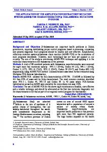
bute that distinguishes them from other spatial features. Building roofs often are homogenous objects that can be segmented from other image features. Homogeneity is a scale-dependent attribute, but for small-scale images (1:4000), roof regions often appear homogeneous. However, utility pipelines and ducts can disturb the building roof homogeneity. Texture is another problem that can decrease the ability to segment building roofs. To account for these problems, several modifications are proposed to the original split-and-merge algorithm. The algorithm presented differs from the conventional split-and-merge algorithm in its capability to join neighboring regions based on their intensity and size differences and in its potential for detecting and filling region gaps. The segmentation process is implemented as follows. The image first is divided into smaller regions until a homogeneity condition is satisfied. This is implemented by constructing a quadtree of the image, progressing down the tree, splitting as necessary when inhomogeneities exist. Then a merging algorithm is implemented. The merging is carried out in two steps. Adjacent regions are first merged based on the differences between the minimum and maximum intensities. Large regions then are merged with their small neighbors if the differences in their intensities are smaller than a given threshold. Intensity thresholds for splitting and merging range between 10 and 15, while the size threshold is kept fixed relative to the image size. One of the problems noticed after segmenting the image is the presence of holes inside the segmented regions. This can occur because of texture and/or utility features. Holes are detected and removed as follows. First for each region its pixels are located and copied to a template image with a background intensity of
(a)
(b)
(c)
Figure 1. Split-and-merge segmentation results for the image of one building: (a) original image, (b) image after splitting, (c) final regions
zero. A region-growing algorithm then is used to connect all the pixels that do not belong to either the background or the region. These pixels are described as holes and are attached to the original region. Another problem also observed in the results is the splitting of some roof patches into two or more regions. To overcome this problem, an average intensity is computed for each region and any two neighboring regions are merged if the difference between their average intensities is smaller than a given threshold, regardless of their sizes. Small regions, very dark regions, and very bright regions are eliminated. Thresholds for the region merging and elimination are kept fixed relative, at this stage, to the intensity range of the images and the image size. The results of the segmentation process for one sample building are shown in Figure 1. Figure 2 shows the results of segmenting the images of five other buildings.
Region Classification Buildings usually are elevated blobs in the DEMs. On the other hand, building regions possess linear borders. Other features such as trees also are elevated; however, they do not have linear borders. Roads and sidewalks have linear borders, but are not elevated. Therefore, in this research the high elevation and border linearity attributes are used to discriminate building roof regions from other regions using a neural network. Each image region is assigned two attributes for the discrimination process. The first attribute measures the linearity of the region boundaries, while the second attribute measures the percentage of the points in the region that are above a certain height. Border linearity is measured using a modified version of Hough transformation (Hough 1962). First, border points are extracted and sorted so they traverse the border clockwise. For each border point, the previous five points and the next five points are found to form a local line at each point. The adjusted line parameters (αa, Pa) and the quadratic form of the residuals for the local line at each point are computed using the least-squares estimation technique. The algorithm is implemented in three runs at each point; the first run is when the point is in the middle of the line; in the second run, the local line is shifted so that the point is at the end. In the third run, the local line is shifted so that the specified point is the first point. If the minimum quadratic form value is small, the parameter space cell at the location of the local line parameters, i.e., αa, Pa, is increased by one. The parameter
(a) (b) Figure 2. Split-and-merge segmentation results for the images of five buildings: (a) original images, (b) final regions URISA Journal • Elaksher, Bethel
7
(a)
(b) Figure 3. The parameter space for a roof region (a) and a nonroof region (b)
(a) (b) Figure 4. DEM (a) and DSM (b) for an area with several buildings, same vertical scale
space then is searched and analyzed to determine a measure for border linearity. Border linearity is measured as the percentage of the number of points in the larger four cells to the total number of border points. Figure 3 shows a parameter space for a roof region and another parameter space for a nonroof region. A digital elevation model (DEM) is used to quantify the height of each region. First, the digital surface model (DSM), i.e., representing bare ground, is extracted. Minimum filters are used to perform this task (Masaharu and Ohtsubo 2002, Wack and Wimmer 2002). The filtering process detects and consequently removes points above the ground surface to recognize high points in the data set. The minimum filter size should be large enough to include data points that are not noise. However, iterative approaches could be used to avoid the effect of noise. In this research, the size of the filter is 9x9 pixels. The filtering is 8
repeated iteratively until the DSM is extracted. The differences between the DEM and the DSM then are computed and used to represent height information. The use of the height information in preference to the elevations makes the algorithm applicable for both flat and slope terrains. Figure 4 shows the DEM and DSM of an area with several buildings. Each point in the image then is assigned a height value by projecting the differences between the DEM and the DSM back to the image using the image registration information, the pixel location in the image, and the DEM elevation. For each image point a ray is generated, starting from the exposure station of the camera and directed toward the point. The intersection between the ray and the DEM defines the location of the corresponding DEM post. The height information at this location then is used as the height of the corresponding image point. The region height URISA Journal • Vol. 20, No. 1 • 2008
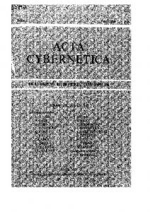
measure is defined as the percentage of the number of points in the region that are above a certain height to the total number of points in the same region. The neural network implemented in this research is a feedforward back-propagation network (see Figure 5). The network consists of three layers: an input layer, one hidden layer, and an output layer. The number of neurons in the first layer is two. The number of neurons in the second layer is selected to be ten. The number of neurons in the third, i.e., last, layer is one. The output of this neuron is either one in case the region is a roof region or zero in case the region is not a roof region. The activation function for all neurons in the first and second layers is the sigmoid functions (Principe et al. 1999). For the output neuron, the step function is chosen as the activation function. To study the performance of the neural network, a variety of training data sets are used with different sizes: 20, 50, 100, 200, and 400 samples, including 2, 5, 10, 20, and 40 roof samples, respectively, while the other samples are nonroof samples. The average detection rate and false alarm rate for each training data set is recorded and shown in Figure 6. Results show that increasing the size of the training data set does not affect the detection rate significantly. However, increasing the size of the training data set does have a significant effect on the false alarm rate.
Image Polygon Extraction The two-dimensional modified Hough space is utilized in extracting the borderlines for the roof regions. Given all points contributing to a certain cell, a nonlinear least-squares estimation model is used to adjust the line parameters of that cell. Lines then are grouped recursively until no more lines with similar parameters are left and short lines are rejected. The next step is to convert the extracted lines to polygons via a rule-based system. The rules are designed as complex as possible to cover a wide range of polygons. The mechanism works in three steps. The first step is to find all the possible intersections between the borderlines. However, if two lines are almost parallel, i.e., intersecting angle out of the range (30o—150o), the intersection point is not considered. The next step is to generate a number of polygons from all recorded intersections. Each combination of three and four intersection points is considered a polygon hypothesis. Hypotheses are ignored if the difference in area between the region and the hypothesized polygon is large. The best polygon that represents the region is chosen from the remaining hypotheses using a template-matching process. The template is chosen to be the region itself, while it is matched across all polygon hypotheses. The hypothesis with the largest correlation and minimum number of vertices is chosen to be the best-fitting polygon. The extracted polygons for six sample buildings are shown in Figure 7. This algorithm succeeded in overcoming several limitations of the segmentation process, such as partially occluded regions, overshooting and undershooting borders, and incomplete regions. This is observed by comparing Figures 1, 2, and 7.
Three-Dimensional Polygon Extraction Polygon Correspondence Figure 5. The implemented neural network
After extracting the building roof polygons from the images, polygon correspondence should be established. A new technique to find corresponding polygons based on their geometrical properties
(a)
(b) Figure 6. The detection rate (a) and the false alarm rate (b)
URISA Journal • Elaksher, Bethel
9
Figure 7. Extracted image polygons for six sample buildings
Figure 8. The roof vertices of one building, before reconstructing the roof topology
Figure 9. The roof vertices of one building, after reconstructing the roof topology
is developed and presented in this section. All possible polygon corresponding combination sets are considered, and for each combination a correspondence cost is computed. The computed cost is used to determine the best corresponding polygon set. First, the coordinates of each two-dimensional polygon center are computed from the coordinates of its vertices. All possible polygon correspondence combinations are exhaustively enumerated and considered, and for each combination the polygon centers are matched across all available views. Because more than one pair of images is available, a function of the residuals of the image coordinates can be calculated and used as the matching cost. For each combination of four polygons, four collinearity 10
equations (Mikhail et al. 2001) can be written using the leastsquares estimation technique. After determining the object space coordinates of the intersecting point, the quadratic form of the residuals is computed. If the four polygons across all views are corresponding, then the quadratic form should be small, otherwise it would be large. Therefore the quadratic form for each polygon correspondence set serves as its cost. A four-dimensional array is constructed to store the corresponding cost values. The array dimension is the same as the number of images. Each axis in the array represents the polygons of one image. The residual cost value is stored at the corresponding location in the four-dimensional array. The axis with the largest number of polygons is used as the reference axis and for each polygon on this axis; its subspaces array is used to find its corresponding polygons in the other images. This subspace array is searched and its minimum value defines the corresponded sets. The minimum value indexes for the subspace array are used as the corresponding polygons in other images. If a polygon corresponds to more than one set, the total residual cost is used to solve such cases.
Computing the Three-Dimensional Polygon Coordinates After finding the corresponding polygons, the three-dimensional coordinates of each roof polygon center are computed; however, the correspondence problem between the polygon vertices is not solved. To solve this problem, another least-squares adjustment model is implemented. The input observations are the image coordinates of the polygon vertices and the unknowns are the object space coordinates for the three-dimensional polygon vertices. To solve the correspondence relations between the vertices within a group of corresponding polygons, the following process is implemented. For each polygon correspondence set, all vertex combinations are considered, and for each combination, the threedimensional coordinates for the polygon vertices are computed. Each set includes a number of subsets (three subsets for triangles and four for quadrilaterals); each subset includes a group of hypothesized matching vertices. The quadratic form is computed for each subset, then they are added to create the total residual URISA Journal • Vol. 20, No. 1 • 2008
of the set. The quadratic forms of the sets then are compared and the set with the minimum quadratic form is selected.
Roof Topology Reconstruction After finding the corresponding vertices, the three-dimensional coordinates for each vertex are computed; however, the building topology is not yet constructed as shown in Figure 8. A geometrically constrained least-squares model is implemented to refine the locations of the polygon vertices and to construct the building topology. The input observations are the image coordinates of the polygon vertices; the unknowns are the object space coordinates for the three-dimensional vertices. The aim of this step is to convert groups of neighboring vertices into one vertex, adjust the elevations of horizontal points, and reconstruct the correct relation between adjacent polygons. The following constraints are used: 1. Nearby vertices should be grouped into one vertex: The resultant vertices from the previous step need to be grouped, as shown in Figure 8, for the extracted three-dimensional polygons may not be contiguous. This results in having more than one point in the position of a single roof vertex. If the distance between any two or more vertices is smaller than a fixed threshold (0.50 meter), their coordinates are constrained to be equal. 2. The polygon vertices should be planer: It is assumed that complex building roofs are built up from planar surfaces. The aim of this constraint is to force the vertices of any polygon to lie in the same plane. This constraint is used only if the number of vertices in the polygon is larger than three. 3. Points that are almost in a horizontal plane are constrained to have the same elevation: If a group of points has a small difference in elevation (0.10 meter), they are constrained to have the same (Z) coordinate. 4. Symmetric polygons should be constrained to have symmetric parameters: If the computed parameters for any two planes indicate that the two planes are approximately symmetric, the two planes are constrained to be symmetric. Thresholds for applying the constraints are fixed for all buildings. The results of this step are shown in Figure 9.
Building Topology Reconstruction After determining the topology of the roofs, the last step is to reconstruct the perimeter facets. This is achieved by the following algorithm. First, border vertices are determined, using a point in polygon algorithm, and sorted clockwise. A facet is generated for any two successive border vertices. The two vertices are assumed to be the upper points of the facet. The horizontal coordinates of the lower two points are taken exactly as the horizontal coordinates of the upper two points, while the elevations are automatically measured from the nearest DSM post.
Results A sample of 30 buildings extracted using the presented algorithm is shown in Figure 10. The results show the completeness and URISA Journal • Elaksher, Bethel
Figure 10. The wireframes of the extracted buildings (repositioned)
accuracy of the three-dimensional buildings that can be extracted using the presented system. To evaluate the accuracy of the extracted buildings, the three-dimensional coordinates of the extracted building vertices were extracted manually and compared with the automatically extracted coordinates. The average rootmean-square errors for the horizontal and vertical coordinates of all building vertices are 0.30 meter and 0.40 meter. Out of about 150 roof regions, 141 roof polygons were detected.
Discussions and Conclusions This paper presents a new algorithm to generate high-quality three-dimensional building information. Results show the great improvement that the algorithm adds. The user only has to select an image patch for the building in the first image. The algorithm utilizes radiometric and geometric properties of urban build11
ings. Image segmentations, neural networks, rule-based systems, photogrammetric mathematical models, and rigorous geometric constraints are used. The paper shows that at the employed image scale (1:4000), segmentation provides high-quality image regions that can be used in the building extraction process. The DEM is only used to provide evidence about the height of the regions. The DEM is generated from the same data set and the only requirement on its quality is that at least one DEM post is inside each roof region. Regions are classified using border linearity and region height. Classification results show that these attributes are adequate to discriminate roof regions. However, other attributes, such as color, could be used. Although the rule-based system extracted either triangle or quadrilateral roof patches, the system could be used to extract any roof shape. The rigorous photogrammetric mathematical models succeeded in finding conjugate polygons, simultaneously matching across several views, and implementing the constraint equations for topology reconstruction. Although several thresholds are used, their values were fixed for all buildings, except the intensity difference threshold that ranged from 10 to 15. Future work will focus on using color information in the segmentation. The model provided an average RMS of about 0.35 meter. With comparison to the image scale, this represents an average accuracy of three pixels in the image coordinates for the vertices. The algorithm succeeds in extracting a wide range of urban building. The tested data set includes simple buildings with one rectangular roof, gabled roof buildings, multistore buildings with large relief, and a variety of complex buildings.
About the Authors Ahmed F. Elaksher is an assistant professor at the engineering faculty at Cairo University. He earned his Ph.D. in August of 2002 from Purdue University. His areas of interest include object recognition, feature extraction, three-dimensional modeling from remote-sensing images, management of spatial information databases, and decision making using GIS, Internet, and wireless technologies. Corresponding Address: Department of Public Works Faculty of Engineering Cairo University Giza, Egypt
[email protected] James Bethel is an associate professor at the School of Civil Engineering, Purdue University. His areas of interest include photogrammetry, remote sensing, data adjustment, and digital-image processing. Corresponding Address: Purdue University School of Civil Engineering 550 Stadium Mall Drive 12
West Lafayette, IN 47907-2051
[email protected]
References Avrahami, Y., Y. Raizman, and Y. Doytsher. 2004. Semiautomatic 3D mapping of buildings from medium scale (1:40,000) aerial photographs. The International Archives of Photogrammetry, Remote Sensing, and Spatial Information Sciences, Istanbul, Turkey, July 2004, XXXV (B3), 774-9. Brunn, A., and U. Weidner. 1997. Extracting buildings from digital surface models, The International Archives of Photogrammetry, Remote Sensing, and Spatial Information Sciences. Stuttgart, Germany, September 1997, XXXII (3-4W2), 27-34. Chein, L., and W. Hsu. 2000. Extraction of man-made buildings in multispectral stereoscopic images. The International Archives of Photogrammetry, Remote Sensing, and Spatial Information Sciences. Amsterdam, The Netherlands, July 2000, XXXIII (B3/1), 169-76. Fischer, A., T. Kolbe, F. Lang, A. Cremers, W. Förstner, L. Plümer, and V. Steinhage. 1998. Extracting buildings from aerial images using hierarchical aggregation in 2D and 3D. Computer Vision and Image Understanding 72, no. 2: 185-203. Förstner, W. 1999. 3D-city models: Automatic and semiautomatic acquisition methods. Photogrammetric Week, Stuttgart (September 1999). Henricsson, O., F. Bignone, W. Willuhn, F. Ade, O. Kubler, E. Baltsavias, S. Mason, and A. Grun. 1996. Project amobe: Strategies, current status, and future work. The International Archives of Photogrammetry, Remote Sensing, and Spatial Information Sciences, Vienna, Austria, July 1996, XXXI (B3), 321-30. Hongjian, Y., and Z. Shiqiang. 2006. 3D building reconstruction from aerial CCD image and sparse laser sample data. Optics and Lasers in Engineering 44, no. 6: 555-66. Horowitz, S. L., and T. Pavlidis. 1974. Picture segmentation by a direct split and merge procedure. In Proceedings of 2nd International Conference on Pattern Recognition, Copenhagen, Denmark, August 1974, 424-33. Hough, P. V. C. 1962. Method and means for recognizing complex patterns. U.S. Patent 3,069,654. Kim, A. 2001. Multi-view 3D object description with uncertain reasoning and machine learning. Ph.D. Thesis, University of Southern California, August 2001. Lari, Z., and H. Ebadi. 2007. Automatic extraction of building features from high resolution satellite images using artificial neural networks. In Proceedings of ISPRS Conference on Information Extraction from SAR and Optical Data, with Emphasis on Developing Countries, Istanbul, Turkey, May 2007.
URISA Journal • Vol. 20, No. 1 • 2008
Lee, D. S., J. Shan, and J. S. Bethel. 2003. Class-guided building extraction from IKONOS imagery. Photogrammetric Engineering and Remote Sensing 69, no. 2: 143-50. Lin, C., and R. Nevatia. 1998. Building detection and description from a single intensity image. Computer Vision and Image Understanding, 72, no. 2: 101-21. Masaharu, H., and K. Ohtsubo. 2002. A filtering method of airborne laser scanner data for complex terrain. The International Archives of Photogrammetry, Remote Sensing, and Spatial Information Sciences, Graz, Austria, XXXIV (3B), 165-9. Mikhail, E., J. Bethel, and J. McGlone. 2001. Introduction to modern photogrammetry. New York: John Wiley and Sons. Morgan, M., and A. Habib. 2002. Interpolation of LIDAR and automatic building extraction. In Proceedings of the 2002 ASPRS, Washington, D.C., April 2002 (on CD-ROM). Muller, S., and D. W. Zaum. 2005. Robust building detection in aerial images. The International Archives of Photogrammetry, Remote Sensing, and Spatial Information Sciences, XXXVI (3/W24), Vienna, Austria, August 2005 (on CD-ROM). Principe, J., N. Euliano, and W. Lefebvre. 1999. Neural and adaptive systems: Fundamentals through simulation. New York: John Wiley and Sons. Rottensteiner, F. 2000. Semiautomatic building recognition integrated in strict bundle block adjustment. The International Archives of Photogrammetry, Remote Sensing, and Spatial Information Sciences, Amsterdam, The Netherlands, July 2000, XXXIII (B2), 463-8. Samet, H. 1982. Neighbor finding techniques for images represented by quadtrees. Computer Graphics and Image Processing 18, no. 1: 37-57.
URISA Journal • Elaksher, Bethel
Shmid, C., and A. Zisserman. 2000. The geometry and matching of lines and curves over multiple views. IJCV 40, no. 3: 199-233. Tarsha-Kurdi, F., T. Landes, P. Grussenmeyer, and E. Smigiel. 2006. New approach for automatic detection of buildings in airborne laser scanner data using first echo only. The International Archives of Photogrammetry, Remote Sensing, and Spatial Information Sciences, Bonn, Germany, September 2006, XXXV (I/3) (on CD-ROM). Theng, L. B. 2006. Semi-automatic building extraction utilizing Quickbird imagery. Journal of Engineering Letters 13, no. 3 (November 2006), http://www/engineeringletters.com/ issues_v13/is sue_3/. Tse, R. O. C., C. M. Gold, and D. Kidner. 2006. A new approach to urban modeling based on LIDAR. In Proceedings of Winter School of Computer Sciences, the 14th International Conference in Central Europe on Computer Graphics, Visualization and Computer Vision, Pilsen, Czech Republic, January-February 2006, 279-86. Wang, S. D., and Y. H. Tseng. 2004. Semi-automated CSG model-based building extraction from photogrammetric images. The International Archives of Photogrammetry, Remote Sensing, and Spatial Information Sciences, Istanbul, Turkey, July 2004, XXXV (B3) (on CD-ROM). Wack, R., and A. Wimmer. 2002. Digital terrain models from airborne laser scanner data—a grid based approach. The International Archives of Photogrammetry, Remote Sensing, and Spatial Information Sciences, Graz, Austria, XXXIV (3B), 293-6.
13
TM
Robust Principal Component Analysis and Geographically Weighted Regression: Urbanization in the Twin Cities Metropolitan Area of Minnesota Debarchana Ghosh and Steven M. Manson Abstract: In this paper, we present a hybrid approach, robust principal component geographically weighted regression (RPCGWR), in examining urbanization as a function of both extant urban land use and the effect of social and environmental factors in the Twin Cities Metropolitan Area (TCMA) of Minnesota. We used remotely sensed data to treat urbanization via the proxy of impervious surface. We then integrated two different methods, robust principal component analysis (RPCA) and geographically weighted regression (GWR) to create an innovative approach to model urbanization. The RPCGWR results show significant spatial heterogeneity in the relationships between proportion of impervious surface and the explanatory factors in the TCMA. We link this heterogeneity to the “sprawling” nature of urban land use that has moved outward from the core Twin Cities through to their suburbs and exurbs. Keywords: Land use, urbanization, robust principal component analysis, geographically weighted regression
Introduction
We have long altered the land by clearing forests, farming, and building settlements. This land change has serious social and environmental impacts, many of which are increasingly evident in urban areas that now host the majority of the world’s population. In the United States, urbanization is driven primarily by suburbanization or decentralized, low-density residential land use, and creation of far-flung suburbs or exurbanization. While suburbanization offers important benefits such as affordable housing, it also has negative impacts on systems ranging from transportation to natural habitat to infrastructure efficiencies to inner-city economies (Burchell et al. 1998, Daniels 1999, EPA 2001). The magnitude and nature of urbanization impacts are tied not only to the amount of land converted to urban use but also to its spatial configuration and pattern (IGBP-IHDP 1995). Dispersed urbanization, for example, creates infrastructure inefficiency by spreading out roads or sewer networks. Despite the importance of spatial patterning in determining impacts of urbanization, a good deal of urban research focuses on aggregate measures such as commute time or population density (Galster et al. 2001). Though this synoptic view is a critical avenue for research, it may not capture the temporal and fine-scaled spatial patterns and processes of urbanization (Hasse and Lathrop 2003). A variety of approaches meet the need to examine and model land use at fine spatial scales, and to these we add a new one. Methodologies range from simple mathematical formulas and gravity models to sophisticated spatiotemporal simulations (Kaimowitz and Angelsen 1998, Lambin 1994, Parker et al. 2003). In this paper, we present a hybrid approach—robust URISA Journal • Ghosh, Manson
principal component geographically weighted regression (RPCGWR)—to examine both the location of urban land use and the relative influence of socioeconomic, demographic, policy, and environmental factors. We integrate two different methods, robust principal component analysis (RPCA) and geographically weighted regression (GWR) to create a novel alternative to standard statistical approaches. First, to reduce the dimensions and number of primary regressors, we applied principal component analysis (PCA) to the explanatory variables. To account for the influence of outliers in standard PCA, we conducted a robust principal component analysis (RPCA) by employing a projection pursuit approach. Second, to capture spatial heterogeneity in the urban landscape, we conducted GWR on the robust principal components (RPCs). We compared the results of the RPCGWR with a standard global principal component regression (RPCGR) and used a series of visual and statistical comparisons to better understand how RPCGWR lends insight into the complex dynamics of urban land use.
Study Area and Background
Urbanization has profound implications for the environmental and socioeconomic sustainability of communities such as the Twin Cities Metropolitan Area (TCMA) of Minnesota (see Figure 1). This 7,700 km2 seven-county area is the economic hub of a multistate region. Home to 2.8 million people, it is forecasted to top 3.5 million by 2020. It is also a major center of sprawl, the rapid expansion of low-density suburbs into formerly rural areas and the creation of urban, suburban, and exurb agglomerations buffered from others by undeveloped land. The metropolitan region also has seen a marked increase in sprawl and associated aspects such as traffic congestion (CEE 1999, Schrank and Lomax 2004). The TCMA is an ideal setting for examining land use. The region exemplifies the spatial and temporal dynamics of urban15
Figure 1. Twin Cities Metropolitan study site and percentage of impervious surface
ization in the United States. It serves as the hub for a large geographic area and stands in relative isolation from other large urban agglomerations, making it easier to extract land-use dynamics at the metropolitan scale. It also is important to understand the role of the region’s distinctive policy setting in shaping land-use patterns because jurisdictions nationwide are wrestling with the balance between local laissez-faire dynamics and tightly controlled regional development (Pendall et al. 2002).
Methodology
Urban researchers and policy makers have long used statistical regression analysis to understand factors important to urbanization. This approach creates a mathematical model of the relationship between some measure, termed the response variable, and a series of explanatory variables. In the case of the TCMA, we can assess the relationship between urbanization in a given location (percentage of impervious surface) as a function of potential environmental, socioeconomic, and demographic factors, and policy variables for that location (measured by the explanatory variables). We expanded on this general approach by using robust PCA (RPCA), which acts on the large number of explanatory variables to create several key robust principal components (RPCs) that serve as composite variables (Li 1985). We then conducted geographically weighted regression (GWR) with the RPCs to capture spatial heterogeneity in the relationship between urban land use and the selected principal components.
Data We identified a broad slate of explanatory factors important to understanding urbanization in the TCMA through a theoretical analysis of the land-use literature and consultation with experts in the community, in particular the staff of the Metropolitan Council (see Table 1). The council is a comprehensive regional planning framework that coordinates the land-use activities of the region’s 272 local units of government, including 188 townships. Theories of relative space focus on the broader spatial organization of social and environmental factors that affect decision making, particularly through returns to land that vary with their distance to phenomena that, in turn, affect input costs or output prices (e.g., bid-rent Alonso and Von Thünen circles) (Alonso 16
1964, Bockstael 1996). Such phenomena include proximity to employment centers, infrastructure, and locations with aesthetic or recreational value. For the TCMA, of particular importance is access to key infrastructure including sewerage, primary highways, and surface roads. Also critical is cost-distance to the core Twin Cities (Minneapolis and St. Paul), distance to the nearest park, water bodies, shopping centers, and urban agglomeration. We included proximity to airplane noise as a nuisance factor that discourages urban development. Euclidian distance to a feature is denoted (D); for example, SEWERD is distance to the nearest sewerage. We also calculated cost-distance surface to the nearest feature as a function of highways (D1) and surface roads (D2). In this case, we calculated two different cost-distance surfaces that vary according to whether highways or surface streets are used to arrive at the feature of interest. SHOPD1, for example, denotes the cost-distance (measured in time as a function of distance traveled on the network) to the nearest shopping center via highways, while SHOPD2 denotes cost-distance via surface streets. On the other hand, related theories of absolute space consider local neighborhood characteristics such as population density, tax rates, existing land cover, lot size, and school district quality (e.g., the Ricardian view of economic activity) (Bockstael 1996, Irwin 2002). Absolute demographic and socioeconomic factors that bear on urbanization in the TCMA include median income, nonwhite population, population density, school test scores, and prevalence of subsidized school lunches as a measure of neighborhood characteristics (Bayoh et al. 2006, Soliani and Rossi 1992, Vincent 2006). Key political and policy institutions include agricultural and natural areas protection programs, county governments, which control some development costs, and the Metropolitan Council’s Metropolitan Urban Services Area (MUSA), which enforces planned growth policies. Environmental factors include soil quality, bedrock depth, elevation, and slope, which, in turn, affect ease of construction, the potential for aesthetic views, and competition for land. Table 1 includes the variable name, description, and data sources for all the explanatory factors included in the study.
Robust Principal Component Analysis (RPCA)
We used an RPCA to reduce the number of explanatory variables examined in the GWR. There are two advantages in regressing the response variable (impervious surface) against RPCs rather than directly on the explanatory variables. First, explanatory variables often are highly correlated with one another (multicollinearity), which may cause inaccurate estimations of regression coefficients or poorly behaved covariance matrices when estimating a standard regression model. One solution to this problem, dropping variables, can be at odds with the need to keep theoretically valid and distinct explanatory variables in the model, such as distance to parks and distance to water, which are conceptually separate but often highly correlated. Because the RPCs are uncorrelated, multicollinearity can be avoided by using the RPCs in place of URISA Journal • Vol. 20, No. 1 • 2008
Table 1. Response and explanatory variables in the study
Variables
Description Impervious surfaces in the TCMA TCMAIMP (dependent variable) Enrollment in the agricultural proAGRIPROT tection program BEDROCK Bedrock height County (7 counties, dummy variables) COUNTY ELEV Elevation Highway, cost-distance to nearest HWYD1 via main freeways Highway, cost-distance via surface HWYD2 streets Median income by census block INCOME group Airport 65db noise contour, disMAC1995D tance to (1995) Airport 65db noise contour, disMAC2006D tance to (2006) Minneapolis, cost-distance to via MPLSD1 main freeways Minneapolis, cost-distance to via MPLSD2 surface streets MUSA Metropolitan Urban Services Area Nonwhite population by census NONWHITE block group PARKD1 Park, cost-distance to nearest via main freeways Park, cost-distance to nearest via PARKD2 surface streets Population density by census block POP group (persons/km2) PROTECTD Protected areas, distance to nearest SCHENG English test scores, by school district Subsidized lunch programs, by SCHLNCH school district (%) SCHMATH Math test scores, by school district SEWERD Sewerage, distance to nearest Shopping center, cost-distance to SHOPD1 nearest via main freeways Shopping center cost-distance to SHOPD2 nearest via surface streets SLOPE Slope SOIL Soil types (3 types, dummy variables) STPAULD1 STPAULD2 TCD1 TCD2 WATERD
St. Paul, cost-distance to via main freeways St. Paul, cost-distance to via surface streets City, cost-distance to via main freeways City, cost-distance to nearest via surface streets Water body > 3 acres (distance to)
Source* MC MC MC NHGIS DNR MC MC NHGIS MAC MAC MC MC MC NHGIS DNR, DOT DNR, DOT NHGIS MC MC MC MC MC MC MC MC DNR, USGS MC MC MC MC DNR
*Metropolitan Airports Commission (MAC), Metropolitan Council (MC), Minnesota Department of Natural Resources (DNR), Minnesota Department of Transport (DOT), National Historical GIS (NHGIS), Remote Sensing and Geospatial Analysis Laboratory (RSGAL), and U.S. Geological Survey (USGS)
URISA Journal • Ghosh, Manson
the original explanatory variables. Second, extracting a subset of RPCs for prediction reduces the dimensionality of the regressors. In the case of the TCMA, ongoing collaboration with local officials and researchers has identified a large number of potential explanatory variables (see Table 1). Thus, we used an RPCA to reduce the dimensionality of the problem—the number of explanatory variables—and accommodate for multicollinearity. Classical PCA is vulnerable to outlying observations. As even a single large outlier can heavily influence the parameter estimates of PCA, we used a method termed projection pursuit, or the notion that while most projections (combinations of derivatives of data) are of low-order complexity or largely normal Gaussian distribution, a few combinations or derivatives will offer far-from-Gaussian distributions or high-order complexity (Croux 1996, Li 1985). For given observations x1,…..,xn Є IRp, collected in the rows of the data matrix X, a coefficient vector b Є IRp is defined for one-dimensional projection of the data. We assume that the first k – 1 projection directions y1,……,yk – 1 (eigenvectors) ( k > 1) have already been measured. For finding the kth eigenvalue, a projection matrix is defined as
(1) for projection on the orthogonal complement of the space spanned by the first k – 1 eigenvectors (for k = 1 we can take P = I p). The kth eigenvector then is defined by maximizing the k function b ® S (X P kb) under the conditions b T b. To extract RPCs, we have to select a subset k < p of components through a three-part process. First, through sequential selection, we include k RPCs that explain approximately 90 percent variation of the data set. Second, we select k RPCs with eigenvalues greater than one. Third, we analyze the “scree plot,” which graphs the eigenvalues (expressed as explained variance) by each RPCs as a line diagram (detailed later in this paper).
Geographically Weighted Regression of Robust Principal Components
With the selected k RPCs, we conducted a geographically weighted regression (GWR) analysis of land use. GWR offers a number of advantages over standard regression. A typical leastsquares regression model of the form:
(2) is a “global” regression, which assumes that the relationship between the explanatory variables and the response variable is constant everywhere in the study area. In many situations, this is not necessarily true, especially with spatial varying variables. GWR extends the traditional global regression framework (equation 2) by allowing local rather than global parameters to be estimated. In this case, the model in equation 2 is rewritten as: 17
(3) where (ui, vi) denotes the coordinates of the ith point in space and βk (ui,vi) is a realization of the continuous function βk (u,v) at point i. Equation 3 creates a continuous surface of estimated parameter values, and measurements of this surface are taken at certain points to denote the spatial variability of the surface. This spatial variability is estimated through the geographical weighting scheme, W(ui, vi), defined such that data points nearer to (ui, vi) will be assigned higher weights in the model than data points farther away. That is,
(3) where the bold type denotes a matrix that represents an estimate of , and W(ui, vi) is an n by n matrix whose off-diagonal elements are zero and whose diagonal elements denote the geographical weighting of each of the observed data for regression point i (Fotheringham 2002). The resulting parameter estimates then can be mapped to analyze local variations in the estimated parameter relationships. Various diagnostic measures further increase the analytical capability of GWR, such as the Akaike Information Criterion (AIC), local standard errors, local measures of influence, and local goodness of fit. As examined later on, the parameter estimates also are tested for evidence of significant spatial variation relative to the global model. Figure 2 summarizes the steps involved in the methodology in a schematic diagram.
Figure 2. Schematic diagram showing methodological framework
18
Results and Discussion
As mentioned previously, we engaged in a three-step process. We first extracted RPCs, and analyzed component loadings and clustering of initial explanatory variables in the component space. Second, we used the RPCs in a standard global regression in what we term a robust principal component global regression (RPCGR), where we model the response variable, proportion of impervious surface, against the selected RPCs. Third, we examined differences between the results of RPCGR and a robust principal component geographically weighted regression (RPCGWR). We used the GWR 3.0 software package (Fotheringham 2002) and R statistical software (Robust PCA and Projection Pursuit, pcaPP package) for statistical analysis and Arc GIS 9.1 (ESRI) for calibrating the RPCGWR model components and visualization of the results.
Table 2. Total variance explained by the robust principal components
Principal Component
Eigenvalue
Variation (%)
Cumulative Variation (%)
1
7.32
74.80
74.80
2
1.10
13.07
87.87
3
0.45
4.72
92.59
4
0.41
2.89
95.48
5
0.22
1.96
97.44
6
0.15
1.01
98.45
7
0.09
0.63
99.08
Figure 3. Scree plot for RPCA on TCMA variables
URISA Journal • Vol. 20, No. 1 • 2008
Robust Principal Component Analysis Results RPCA using the projection pursuit approach extracted three underlying dimensions from the 30 explanatory variables expected to influence urban development in the TCMA (see Table 1). Table 2 shows both the eigenvalue and the raw and cumulative percentage of variance explained by the extracted RPCs that account for 99 percent of the total variation. The first three RPCs account for 93 percent of the total variation. The first explains 75
Table 3. Explanatory variable loadings onto individual selected robust principal components
Variable
PC1
PC2
PC3
AGRIPROT
0.000
0.000
0.000
BEDROCK
0.000
0.000
-0.002
COUNTY
0.000
0.000
0.000
ELEV
0.000
0.000
0.000
HWYD1
0.222
0.098
-0.379
HWYD2
0.217
0.121
-0.384
INCOME
-0.070
0.976
0.058
MAC1995D
0.211
0.054
0.508
MAC2006D
0.209
0.052
0.52
MPLSD1
0.323
0.069
-0.255
MPLSD2
0.488
0.038
-0.178
MUSA
0.000
0.000
0.000
NONWHITE
0.001
0.002
0.002
PARKD1
0.056
-0.003
-0.107
PARKD2
0.055
-0.007
-0.096
POP
-0.009
-0.011
-0.003
PROTECTD
0.000
0.000
0.000
SCHENG
0.000
0.000
0.000
SCHLNCH
0.000
0.000
0.000
SCHMATH
0.000
0.000
0.000
SEWERD
0.127
-0.002
-0.083
SHOPD1
0.266
0.032
-0.253
SHOPD2
0.312
-0.037
-0.157
SLOPE
0.000
0.000
0.000
SOIL
0.000
0.000
0.000
STPAULD1
0.34
0.029
-0.137
STPAULD2
0.538
-0.064
0.178
TCD1
0.333
0.048
-0.21
TCD2
0.418
-0.019
-0.049
WATERD
0.012
-0.016
-0.022
URISA Journal • Ghosh, Manson
Figure 4. Variables in three-dimensional component space
percent, the second 13 percent, and the third explains 5 percent of the variance (see Table 2). There is, therefore, a steep drop in the percentage of explained variance after the first RPC. This drop also is evident in a scree diagram, which plots the eigenvalues (variances) of the RPCs on the y-axis against the RPC number on the x-axis (see Figure 3). The term scree refers to the fact that the explained-variance curve resembles the side of a mountain with a scree, or rock debris, at the base. When read left to right across the abscissa, this plot shows a clear separation between RPCs with high-explained variance versus low-explained variance. The point of separation is termed the elbow for obvious reasons that nonetheless invite a justified charge of mixed metaphors. In concordance with Table 2 and Figure 3, the first RPC explains the large majority of variation, the second less so, and the third a small amount. The elbow occurs at the third RPC, indicating the separation of the most important RPCs from less important RPCs, namely the fourth onward. Thus, we retained the first three RPCs as explanatory variables for further analysis. The key opportunity, and challenge, of PCA is determining what the components actually mean in a real-world setting. Component loadings indicate the relative contribution of the variables to each component (seeTable 3). In addition to examining the degree of correspondence between components and individual variables (Table 3), we also can look for clustering in component space. Figure 4 is a threedimensional graph that shows the position of explanatory variables with high component loadings in the component space. The graph identifies how these variables relate to both the principal 19
Figure 5. Cost-distance factor (RPC1) Figure 7. Infrastructure factor (RPC3)
Figure 6. Income factor (RPC2)
components and other input variables. The first component, RPC1, has a number of variables with high loadings. The variables, in descending order, are cost-distance surfaces by the second-order roads to St. Paul (STPAULD2), Minneapolis (MPLSD2), and to the nearest of the two cities (TCD2). These are followed by cost-distance surface by first-order roads to St. Paul (STPAULD1), Minneapolis (MPLSD1), and to the nearest of the two cities by highways (TCD1). The seventh and eighth variables are the two cost-distances to the nearest shopping center by highway and surface streets (SHOPD1 and SHOPD2). These variables are positively related to RPC1, or, in other words, observations with higher values of RPC1 also will indicate higher values of all the variables mentioned previously and vice versa. Because these variables measure cost-distances to key urban centers, markets, and infrastructure, we termed RPC1 as the cost-distance factor. Figure 5 illustrates the spatial variation of the cost-distance factor (RPC1) in the TCMA region along with the explanatory 20
variables that load highly onto this component. Figure 5b shows the influence of cost-distances to the Twin Cities and major shopping centers. The cost-distance factor is least near the center or the two central business districts (CBDs) of the TCMA and increases gradually outward from the center to the suburbs and then to the outer suburbs. Not surprisingly, the initial cost-distance variables also show a similar spatial pattern (see Figure 5a). The second component, RPC2, has median income by block group (INCOME) with a very high component loading of 0.976, almost double that of any other variable/component loading combination. INCOME is positively related to RPC2, indicating that higher values of RPC2 are associated with higher values of INCOME, leading us to term RPC2 as the “income factor.” Figure 6 demonstrates the strong correspondence in spatial variation between the initial variable, INCOME (Figure 6a), and the income-factor, PC2 (Figure 6b). Other indicators that often (but not always) map onto socioeconomic status and neighborhood characteristics, such as school lunch programs or ethnicity, are almost completely subsumed by INCOME. The third component, RPC3, captures a more complicated situation than those associated with RPC1 and RPC2. Unlike the other components, RPC3 has both high positive and negative loadings (see Figure 7). The two strongest positive loadings are past and present distance to the airport 65db noise contour (MAC1995D, MAC2006D), followed by a lower loading on cost-distance to St. Paul via surface streets (STPAULD2). The remaining variables have small negative loadings on PC3. These include cost-distances to the nearest highway (HWYD1 and HWYD2), cost-distances to Minneapolis (MPLSD1 URISA Journal • Vol. 20, No. 1 • 2008
Table 4. Global robust principal component regression (RPCGR) analysis results
Parameter Intercept PC1 PC2 PC3
Coefficients Value 16.033 -4.852 -2.356 1.601
Std. Error
T-Value
0.566 0.146 0.247 0.416
28.346 -33.119 -9.530 3.847 Figure 8. Spatial variation in influence of cost-distance factor (RPC1)
and MPLSD2), cost-distances to the nearest shopping center (SHOPD1 and SHOPD2), cost-distances to the nearest of the two cities (TCD1), and cost-distance to the nearest park via surface streets (PARKD2). RPC3 is more difficult to interpret than the first two components because of the small amount of variance explained by RPC3 and the mixed nature of explanatory variables contributing to it. Although it is not immediately obvious from the loadings on this component, we define PC3 as the “infrastructure factor,” because as will be explored in the following section, this factor captures path-dependence on urban form exerted by exiting infrastructure.
Robust Principal Component Global Regression (RPCGR) We used the three RPCs as explanatory variables in a robust principal component global regression (RPCGR) to form a basis for comparison to robust principal component geographically weighted regression (RPCGWR). Table 4 shows the results of a standard multiple linear regression model (again, termed a global model to distinguish it from GWR). We estimated the model (and the RPCGWR that follows) with 7,000 observations sampled across the TCMA. The RPCGR model is significant for all components (R2 = 0.217, p > 0.01 for PC1-PC3). The proportion of impervious surface in TCMA is negatively related to the cost-distance factor (RPC1) and income factor (RPC2) but positively related to the infrastructure factor (RPC3). Regions with a higher proportion of impervious surface have lower values of the cost-distance factor and the income factor. In contrast, the association between RPC3 and impervious surface is positive; as PC3 increases, the percentage of impervious surface also increases. The global regression model explains only 22 percent of the variance in the percentage of impervious surface as a function of the RPCs, which indicates that the model does not account for all the factors influencing urban development in the TCMA. Beyond missing variables, however, the low explained variance also can be attributed at least in part to the fact that the estimated parameters represent global averages of relationships between impervious surface and the RPCs that may exhibit spatial variation (Fotheringham 2002). In other words, some of the unexplained variance may be associated with the assumption of spatial stationURISA Journal • Ghosh, Manson
arity underlying the global regression model. Theories of relative space, mentioned previously, contend that the intensity of urban development declines with increasing distance from central cities, in this case, Minneapolis and St. Paul. While the global regression identified this relationship between urban development and distance from a central city, it may fail to identify local variations in the power of this relationship. Thus, if the relationship between an explanatory variable and urban development is spatially nonstationary, then the global multiple regression approach can misspecify the actual relationship (Fotheringham 2002). One approach for analyzing these local variations is RPCGWR.
Robust Principal Component Geographically Weighted Regression As noted previously, we term the combination of RPCA and GWR as robust principal component geographically weighted regression (RPCGWR). To assess the effectiveness of RPCGWR, we compared its performance to that of global regression analysis with the same variables, proportion of impervious surface versus the three RPCs that in turn condensed 30 explanatory variables shown in Table 1. With GWR, the parameter estimation at any of the sample observations depends not only on the input data but also on the kernel (model form) chosen and the kernel’s bandwidth (spatial extent of the sample). We used a Gaussian model because the response variable is continuous. The bandwidth was optimized as a part of the GWR calibration using the AIC method, which balances the complexity of the estimated model (defined by how specific the bandwidth becomes) with the extent to which the model fits the data (defined by explained variance). GWR uses a Monte Carlo simulation to test the following hypotheses: (1) whether the data may be described by a GWR model rather than a stationary one and (2) whether individual regression coefficients are stable over geographic space (Fotheringham 2002). A comparison of regression parameters illustrates that RPCGWR outperforms RPCGR for this study. The AIC is reduced from 64,554.63 for the global regression model to 63,871.10 for the RPCGWR model, where a lower AIC indicates a more efficient model. RPCGWR has an R2 of 0.49, which is reasonably high, especially compared to an R2 of 0.22 for RPCGR. RP21
CGWR also has a much lower residual sum of squares (284,179 versus 3,282,543). Finally, we can compare RPCGWR against RPCGWR via an ANOVA, where an F of 6.69 at the p < 0.01 level indicates that RPCGWR significantly improves on the global regression model. In spatial terms, the Monte Carlo test of the local estimates for each of the three RPCs (cost-distance, income, and infrastructure factors) indicates significant spatial variation for a bandwidth of approximately three miles. The spatial pattern of the estimated cost-distance factor (RPC1) is shown in Figure 8. Areas marked by higher absolute values indicate regions where the explanatory variables with higher component loading under RPC1 have a greater influence, while areas of lower values indicate where the explanatory variables are less influential. As noted previously, the global relationship between RPC1 and the proportion of impervious surface is negative, which suggests that urban development is more likely to occur closer (lower costdistance) to the major cites of St. Paul and Minneapolis, either considered singly or in terms of whichever is closest to a given location (STPAULD1/2, MPLSD1/2, and TCD1/2, respectively), the nearest shopping center (SHOPD1/2), or highway (HWYD1/2). RPCGWR shows that the contribution of RPC1 parameter in the regression equation varies over the study region, including a change in sign from negative to positive, which indicates that this relationship is more complex than is suggested by the global regression results. We can assess the statistical significance of the spatial variation by examining t-values at the observations. Values falling beyond 1.96 (i.e., the 95 percent confidence interval) are considered significant (Fotheringham 2002). According to this rubric, there are several areas in the TCMA where a significant positive relationship exits between impervious surfaces and the cost-distance factor. Figure 8b identifies the areas of the TCMA
in which the range of values in Figure 8a constitute significant spatial variation. Areas of particular significance are located in Anoka and Washington counties in the northwest and Carver and Scott counties in the southwest (also see Figure 1). This said, within these counties, there are areas where the inverse is true, particularly northern Anoka County, central Carver County, and northwestern Washington County. These subareas show development in the suburbs away from the CBD and Twin Cities and confirm the “sprawling” nature of urbanization in the TCMA. The global relationship between the proportion of impervious surface and the income factor (RPC2) is significantly positive. Figure 9a shows that this positive relationship holds over most of the study area because the majority of the local parameters also are positive. However, as we move away from the central region of the TCMA to the peripheral regions, especially in the northwestern corner of the Washington County (Figure 9 and Figure 1) and the inner-city region of the Twin Cities of Minneapolis and St. Paul, the relationship becomes negative. This negative relation of income factor and percentage of impervious surface highlights a typical inner-city scenario witnessed in almost all metropolitan regions of the country. Growing population, cheap housing policies, and the dense nature of transportation network are some of the factors that changed the land to concrete urban impervious surface but have simultaneously discouraged the reinvestment and redevelopment of older inner-city communities. This creates a situation of “negative growth,” affecting the processes of land use and environment around the metropolitan perimeter. Figure 9b indicates that the negative relation between percentage of impervious surface and the income factor in the inner-city region of the Twin Cities and parts of northwestern Washington County are statistically significant. The spatial pattern of RPC3, the infrastructure factor, is shown in Figure 10a. As noted previously in terms of the load-
Figure 9. Spatial variation in influence of income factor (RPC2)
22
URISA Journal • Vol. 20, No. 1 • 2008
ings on RPC3, there are strong positive association with both the past and present distance to the airport’s 65db noise contour (MAC1995D, MAC2006D) and weak positive associations with cost-distance to St. Paul via surface streets (STPAULD2). Conversely, there are weak negative associations between proportion of impervious surface and cost-distances to the nearest highway (HWYD1 and HWYD2), Minneapolis (MPLSD1 and MPLSD2), nearest shopping center (SHOPD1 and SHOPD2), nearest of the two cities (TCD1), cost-distance to St. Paul via freeways (STPAULD2), and cost-distance to the nearest park via surface streets (PARKD2). An examination of local parameters from RPCGWR, however, shows a distinct spatial pattern in the changing nature of this relationship. PC3 is positively related to impervious surface in the eastern part of Hennepin County, the entirety of Ramsey and Anoka counties, and the northern part of Dakota County (Figure 10a). These regions are characterized by high values of airport noise (MAC1995D, MAC2006D) and low values for cost-distances to infrastructure and markets (HWYD1/2, MPLSD1/2, SHOPD1/2, TCD1). We originally included airplane noise given anecdotal evidence in the TCMA, supported by studies elsewhere (Nelson et al. 2004), that land development is less likely to increase in areas of high noise, limited indirectly through consumer preferences and directly through policy limits on land use. While the negative impact of airplane noise on urban development may be true in many other study areas, the region around the airport on the border between Hennepin and Dakota Counties contained some of the longest settled neighborhoods of the TCMA. These areas and the adjacent suburbs were developed decades before the airport was built in 1962. These areas also contributed to further development of key infrastructure facilities, including rail, tram, and road networks and are home to the highest density of detached single-family dwellings, which, in turn, feature smaller
backyards than elsewhere in the TCMA and an attendant dense street grid and alley network. The spatial patterning of RPC3, while driven in large part by areas of past development that map onto the spatial pattern of airport noise, also reflects negative loadings for several of the cost-distance measures. In particular, the majority of the areas with an apparently negative relationship with cost-distance fall in largely rural areas that lie far from current infrastructure (highways or markets) or in recent suburban developments that boast lower amounts of imperviousness with their large lot sizes and irregular street grids. As seen in Figure 10a, these areas lie in the northern and western parts of the TCMA.
Conclusion
This study has two types of conclusions, specific and applied. The specific conclusions are derived directly from the RPCGWR model and its interpretations in the context of the TCMA. These conclusions contribute to the literature of spatial analysis and modeling of urbanization in geography. On the other hand, the applied conclusions are the inputs to the policy community of the Metropolitan Council, the Minnesota Pollution Control Agency, and other governmental agencies in the TCMA. The following paragraphs will expand on the specific conclusions first, followed by the applied conclusions. We introduce a hybrid approach, RPCGWR, to examine the relationships between urban development, as approximated by impervious surface, and myriad explanatory social and environmental factors in the TCMA. This approach allows us to sift through a large number of potential factors and identify several key composite factors in the form of RPCs. RPCA, in addition to accounting for outliers in the original data set, is useful for reducing the complexity of explanatory variables, as seen in reducing the initial 30 explanatory variables to three robust components
Figure 10. Spatial variation in influence historical high-density factor (RPC3)
URISA Journal • Ghosh, Manson
23
that account for 93 percent of the total variation. It is important to note, however, that RPCA does not have to divorce the components from the original factors, but, instead, can serve as a way of aggregating and understanding relationships among these factors. The first RPC was defined as the costdistance factor because it aggregates cost-distance measures for city centers, the nearest highways, and shopping centers. The second RPC collapses myriad socioeconomic and demographic factors into a single measure, income. The third component tells a more complicated story because, in addition to contributing a small amount of explained variance, it captures the effect of historical infrastructure development in heavily urban areas and relative paucity of infrastructure in other, more rural areas. We then go one step further by using GWR to better understand the spatial variation in the RPCs as such and their relationship with both urban development and the original explanatory factors. We demonstrate that, for the TCMA, RPCGWR outperformed RPCGR as a tool for examining spatially varying relationships. RPCGWR sheds light on how the importance of socioeconomic and environmental factors can vary over space, in essence adding context to theories of land use by highlighting areas where these factors play out differently. This approach also identifies areas for further investigation. The spatial pattern of the cost-distance component identified areas away from the Twin Cities, for example, where significant positive relationships exist between cost-distances and the proportion of impervious surface contrary to theoretical expectations and trends elsewhere in the region. Similarly, even though the global relationship between the proportion of impervious surface and the income factor (RPC2) is significantly negative, RPCGWR located patches outside the Twin Cities where there is a significant positive relationship between impervious surfaces and income. This spatial heterogeneity is linked to the differences in the nature of urban land use between the core Twin Cities and their suburbs and exurbs. From the application point of view, this work is the first step in developing trajectories of future land change for the Twin Cities. This aspect of the research is tied to the policy community through ongoing consultation with experts from the Metropolitan Council. The mission of this body is to develop, in coordination with local communities, a comprehensive regional planning framework that focuses on transportation and aviation, wastewater treatment and water resources, regional parks, and regional development and infrastructure. Its chief goal is to plan and coordinate efficient and sustainable growth of the metropolitan area. We are exploring two key linkages to the Metropolitan Council. First, we have been working with the Metropolitan Council and the Minnesota Pollution Control Agency, for these agencies find the maps to be useful inputs to hydrology and runoff models and
24
planning future development. Satellite remote sensing provides a cost-effective alternative for obtaining such information when the costs of traditional mapping approaches are increasing and budgets are declining. Second, working with staff at the Metropolitan Council and with the archives maintained by the council, we could identify likely scenarios of growth, tied to population and socioeconomic forecasts, paying particular attention to the role of policy instruments such as zoning, transportation, and infrastructure provision.
Acknowledgments This work is supported in part by the National Aeronautics and Space Administration New Investigator Program in Earth-Sun System Science (NNX06AE85G), the University of Minnesota’s College of Liberal Arts Graduate Research Partnership Program, and the McKnight Land-Grant Professorship Program. The authors gratefully acknowledge the assistance of the editor and anonymous reviewers. Responsibility for the opinions expressed herein is solely that of the authors.
About the Authors Debarchana Ghosh is a Ph.D. candidate in the Department of Geography, University of Minnesota. Her research interests include quantitative analysis, spatial statistics and modeling, GIS, health, and environmental geography. Corresponding Address: University of Minnesota Department of Geography 414 Social Sciences 267 - 19th Avenue South Minneapolis, MN 55455 Phone: (612) 625-6080 Fax: (612) 624-1044
[email protected] Dr. Steven M. Manson is an associate professor in the Department of Geography, University of Minnesota. He combines environmental research, social science, and geographic information science to understand changing urban and rural landscapes in the United States and Mexico. This work is part of his longer-term research on global environmental change, decision making, and understanding complex human-environment systems.
URISA Journal • Vol. 20, No. 1 • 2008
References Alonso, W. 1964. Location and land use. Cambridge, MA: Harvard University Press. Bayoh, I., E. G. Irwin, and T. Haab. 2006. Determinants of residential location choice: How important are local public goods in attracting homeowners to central city locations? Journal of Regional Science 46: 97-120. Bockstael, N. E. 1996. Modeling economics and space: the importance of a spatial perspective. American Journal of Agricultural Economics 78: 1168-80. Burchell, R. W., N. A. Shad, D. Listokin, H. Phillips, A. Downs, S. Seskin, J. S. Davis, T. Moore, D. Helton, and M. Gall. 1998. Costs of sprawl: Revisited. Washington, D.C.: National Academy Press. CEE. 1999. Two roads diverge: Analyzing growth scenarios for the Twin Cities. Minneapolis: Center for Energy and Environment. Croux, C., and A. Ruiz-Gazen. 1996. A fast algorithm for robust principal components based on projection pursuit. In Computational statistics. Heidelberg: Physica-Verlag: 211-16. Daniels, T. 1999. When city and country collide: Managing growth in the metropolitan fringe. Washington, D.C.: Island Press. EPA. 2001. Our built and natural environments. Washington, D.C. Fotheringham, A. S., C. Brundson, and M. Charlton. 2002. Geographically weighted regression—the analysis of spatially varying relationship. West Sussex, England: John Wiley & Sons Ltd. Galster, G., R. Hanson, M. R. Ratcliffe, H. Wolman, S. Coleman, and J. Freihage. 2001. Wrestling sprawl to the ground: Defining and measuring an elusive concept. Housing policy debate 12: 681. Hasse, J. E., and R. G. Lathrop. 2003. Land resource impact indicators of urban sprawl. Applied Geography 23: 159-75.
URISA Journal • Ghosh, Manson
IGBP-IHDP. 1995. Land-use and land-cover change: Science/ research plan. Stockholm: International GeosphereBiosphere Programme and International Human Dimensions Programme. Irwin, E. 2002. The effects of open space on residential property values. Land Economics 78: 465-81. Kaimowitz, D., and A. Angelsen. 1998. Economic models of tropical deforestation: A review. Jakarta: Centre for International Forestry Research. Lambin, E. F. 1994. Modelling deforestation processes: A review. Luxembourg: European Commission. Li, G., and Z. Chen. 1985. Projection-pursuit approach to robust dispersion matrices and principal components: Primary theory and Monte Carlo. Journal of the American Statitstical Association 80: 759-66. Nelson, A. C., R. J. Burby, E. Feser, C. J. Dawkins, E. E. Malizia, and R. Quercia. 2004. Urban containment and central city revitalization. Journal of the American Planning Association 70: 411-25. Parker, D. C., S. M. Manson, M. Janssen, M. J. Hoffmann, and P. J. Deadman. 2003. Multi-agent systems for the simulation of land use and land cover change: a review. Annals of the Association of American Geographers 93: 316-40. Pendall, R., J. Martin, and W. Fulton. 2002. Holding the line: Urban containment in the United States. Washington, D.C.: Brookings Institute. Schrank, D., and T. Lomax. 2004. The 2004 urban mobility report. College Station, TX: Texas Transportation Institute. Soliani, L., and O. Rossi. 1992. Demographic factors and land-use planning in the small islands of southern Europe. Environmental Management 16: 603-11. Vincent, J. M. 2006. Public schools as public infrastructure—roles for planning researchers. Journal of Planning Education and Research 25: 433-37.
25
Where Are They? A Spatial Inquiry of Sex Offenders in Brazos County Praveen Maghelal, Miriam Olivares, Douglas Wunneburger, and Gustavo Roman Abstract: The United States has several laws that restrict the movement of registered sex offenders. The majority of these laws are spatial in nature. However, only a few studies have investigated the use of spatial technology (geographic information system) to analyze the implications of these laws. This study uses GIS to map and identify the offenders who violate the laws policed by federal agencies. Also, the perceived risk because of the sex offenders’ existence in the community is mapped to assist law-enforcement agencies identify the potential suspects when sex crimes are reported. Spatial analysis revealed that more than 50 percent of the offenders resided within the restriction distance of the places where children congregate. Immediate and lateral risk zones were created around each offender to measure the risk each offender brings to the community in which he or she resides. Finally, this study proposes the use of spatial technology to communicate sex-related crimes to increase the awareness of communities at risk of sex-crime victimization.
Introduction
Several studies in the past decade have analyzed sexual abuse on males and females under the age of 18 in the United States (Tjaden and Thoennes 1998, Greenfield 1997). Finkelhor (1994) informed that one in five females and one in seven males are sexually abused by the age of 18. The fear, both personal and altruistic, of becoming a victim of sexual abuse consciously or semiconsciously exists in the community. This fear has been rekindled even more with the recent unfortunate events of sexrelated crimes throughout the nation. In an attempt to redeem neighborhoods of these mishaps, law-enforcement agencies have regulated various sex offender restriction statutes that can help manage the risk posed by sex offenders. While numerous statutes have been in place for about four decades now, the Jacob Wetterling Crimes Against Children and Sexually Violent Offenders Registration Program1 (42 U.S.C. 14071 et seq.) of 1994 reshaped the way law enforcers managed Registered Sex Offenders (RSOs) in the United States. This law required convicted sex offenders to register and notify their law administrators of their movement. Information about offenders such as each offender’s name, age, gender, height, weight, race, and details of the offense are provided to the state authorities such as the State Department of Public Safety. After the death of Megan Kanka at the hands of a convicted sex offender living across the street in New Jersey, President Clinton signed an amendment to this law, requiring all states to make the information about pedophiles and rapists available to the general public (Beck and Travis 2004, Engeler 2005). When this law was signed in May of 1996, the local citizenry was and continues to be informed of the whereabouts of sex offenders in 1. Details of the Jacob Wetterling Crimes Against Children and Sexually Violent Offenders Registration Program can be obtained at the Cornell University Law School U.S. Code collection at http://www.law.cornell.edu/uscode/html/uscode42/usc_ sec_42_00014071----000-.html.
URISA Journal • Maghelal, Olivares, Wunneburger, Roman
their community. This notification system exists in all the states, and makes it mandatory for the offenders to inform the respective state authorities about their movements anywhere in the United States. This information then is made public to notify the communities of the offenders’ details. The Jacob Wetterling act sets minimum standards by federal administration for states. Individual states, on the other hand, can impose more stringent requirements on the offenders. In Texas, the Code of Criminal Procedure, SB1054, Article 42.12, Section 13B (Texas Legislature Online, 78th Legislature) mandates the Child Safety Zone (CSZ) for the state of Texas to be “within 1,000 feet of premises such as school, day-care facility, playground, public or private youth center, public swimming pool, or video arcade facility, places where children generally gather.” Currently, the state of Texas stipulates anywhere from 200 feet to 1,000 feet for this zone, which follows the drug-free zone restrictions used in the state. This study investigates the locations of sex offenders’ residences with respect to the CSZ using a standard 1,000-foot buffer (as mandated by the Texas legislature and currently under discussion in the legislature2) around the child facilities on proximity to an RSO, area of risk owing to the RSO presence, and how such information can be communicated to the general public. The movement of RSOs within and between different states with varying restriction laws makes it difficult for the offenders and the supervising authorities to exactly determine the distance between the residences of the offenders and the CSZ. However, current trends in modern technology such as using a geographic information system (GIS) have made it feasible to closely supervise the mobility restrictions of the registered sex offenders. GIS 2. The existing Texas legislature requires a distance of 1,000 feet. However, the Board of Pardon and the judiciary system can decide this distance case by case. However, Martha Wong, Texas state representative, has moved for an amendment that mandates that all offenders be subjected to a 1,000-foot distance throughout the state of Texas. Details regarding the House Bill 1828 can be found on the Texas legislature Website at http://www.capitol.state.tx.us/.
27
provides a powerful tool to map these locations, efficiently update the data, and frequently check for violators residing in the CSZ. This study uses the current restriction laws stipulated by the Texas legislature to inquire: (1) How many sex offenders reside within the Child Safety Zone (1,000-foot buffer)? (2) how to identify the known offenders in closest proximity to where a victim is reported missing? and (3) how can this digital mapping system help notify and bring awareness to the local community?
Background
Felson and Clark (1998), in their analysis, reported that all crimes are a result of available opportunities. The laws that have been enacted to reduce sex crimes attempt to reduce these opportunities as much as possible. Cohen and Felson (1979) stated that the increase in opportunities of crime is because of the presence of three elements: (1) a suitable target, (2) absence of a guardian, and (3) a motivated offender. This is defined as the Routine Activity Theory (RAT). Therefore, occurrence of sex crimes can be reduced or checked when a guardian is aware of the presence of a motivated offender who may attack a suitable victim. Megan’s Law, in a sense, performs a similar task for society. The law-enforcement agencies inform the respective communities of the presence of a sex offender through the notification system to increase the awareness of individuals living in close proximity to the offender. As a result, these acts help to avoid or reduce the chances of a motivated offender meeting a suitable target in space and time. Extensive literature that analyzes proximity and sex crime are reported in Walker, Golden, and VanHouten (2001). Similarly, to monitor the adjudicated offenders, agencies such as the Parole Board and the Board of Pardon have developed restrictions that control the mobility of the offenders in the community. These restrictions have received wide attention recently. Robertson (2000, 109) suggested that: … an understanding of geographic trends of registered sex offenders, especially as they relate to schools and daycare facilities, may help police narrow their suspect lists in open cases, to those individuals contained within their registration database, living within a close proximity to the victim procurement site, who pose a high risk of recidivism.
Although RAT indicates that there is a relationship between proximity and repeated sex crimes, Levenson and Cotter (2005) reported that there is lack of empirical research in this area. Canter and Larkin (1993) proposed the commuter and marauder hypothesis based on the components of proximity and crime. They proposed that commuters travel to commit crimes in other areas beyond their homes and the marauder criminals use the areas around their homes to commit crimes. Crime and proximity in relation to Child Safety Zone (commuters) has been investigated spatially by Walker et al. (2001). Their study analyzed the proximity of sex offenders and the potential victims using GIS. They used the Arkansas Code of 1,000-foot buffer and identified the offenders who lived within this distance. They also investigated 28
the number of offenders who resided within 1,000 feet from such premises as schools, parks, and day-care centers. In several cases, sex offenders were found to be living in close proximity to the premises where children congregate. Also, just about half of the offenders (47 percent) were reported to be living within the 1,000-foot restriction area. Although the impact of Megan’s Law, though spatial in nature, has not been investigated spatially in relation to proximity and crime (marauder), its effect has been reviewed for its mode of notification by Thomas (2003). His study reported that the methods of disseminating the community notification (Megan’s Law) was through leaflets or flyers, community notification meetings, and other means such as the media, “need-to-know” basis, and marked-car licenses in various communities across the United States. While the exact distance traveled by an offender to commit a sex crime remains to be investigated, Megan’s Law is based on the premise that an individual in immediate and close proximity to a sex offender is at risk of victimization and thus needs to be notified about sex offender presence in the community. In Texas, this act requires notification3 (Texas Criminal Procedures Code Annotated Section 62.201(a)) by mail to households within the zone of influence, defined in two levels depending on the location of the urban or rural setting of an RSO’s dwelling: immediate risk—within three city blocks (or approximately 0.33 miles) in urban or subdivided settings, and lateral risk—within one mile in rural settings (areas outside subdivisions). Conversely, Terry Thomas (2001) reported that the Sex Offender Act of 1997 in the United Kingdom had unforeseen consequences. The implication of this law required setting up a mechanism of registration to help the police decide the risk caused by a dangerous sex offender. This idea of registration of sex offenders was based on three arguments: (1) to help the police identify the suspects after a crime, (2) to prevent crime, and (3) to act as a deterrent (Home Office, 107). The registration laws in United States serve the same purpose. However, residential restrictions for the sex offenders vary from state to state. In Illinois, the least restrictive distance is 500 feet, while California restricts the dwelling of sex offenders within a quarter mile of schools (Levenson and Cotter 2005). Texas law allows these restrictions to vary for each offender, depending on the type of offense committed. Presently, the parole board assigns this distance based on the individual’s offense. This distance can be anywhere up to 1,000 feet. This makes it difficult for the law-enforcement officials to keep a check on the movement of these offenders. To alleviate these difficulties, the Texas legislature has been forwarded a petition to make the restrictive distance of 1,000 feet uniform throughout the state of Texas. Nonetheless, the undisputed fact remains that the primary aim of the notification system is to increase the vigilantism of communities. One of the more recent methods of increasing vigilantism against crime is through Web-based technologies. 3. Details regarding the notification system in Texas are available at http://tlo2.tlc.state.tx.us/statutes/cr.toc.htm, titled “Article 62.201. Additional public notice for individuals subject to civil commitment.”
URISA Journal • Vol. 20, No. 1 • 2008
Spatial technology, in addition to being used as a mapping tool (e.g., Walker et al. 2001, Foote and Crum 1995), can be effectively used as a communication tool using Web GIS. While Web GIS has been used as a communication tool for some time now (e.g., Ramasubramanian 1995), its application to communicate sex crimes has been increasingly advocated (e.g., Albrecht and Pingel 2005, Shyy, Stimson, Western, Murray, and Mazerolle 2005). It is important to communicate information regarding sex crimes because, as suggested by Sampson, Raudenbush, and Earls (1997), it increases the “collective efficacy” of the community. They state that an increase in collective efficacy of a community results in lower expected levels of crime. Therefore, this study provides a methodological approach to identify and notify individuals about the sex offenders in their community using GIS. Deriving from the RAT, sex crime, as a result of proximity, can occur in two ways. In the absence of a guardian by (1) proximity to probable or suitable victims and (2) proximity to motivated offenders. While a detailed literature review by Walker et al. (2001) assesses the issues of proximity to suitable victims using GIS, proximity to motivated offenders has been neglected as a cause of sex crime. The following investigation will help (1) identify the percentage of offenders who violate the residential restrictions if and when 1,000-foot restriction is approved; (2) identify the areas of probable crime in close vicinity to the offenders’ homes; and (3) measure the effectiveness of developing a Web-based GIS notification system that maps the offenders and the restriction zones.
Methodology Study Area The area under study, Brazos County, Texas, has a population of about 152,000 (U.S. Census 2000), comprised of the cities of Bryan, College Station, and Wellborn. About 88 percent of the population of Brazos County resides in the twin cities of Bryan and College Station. The Texas Department of Public Safety (TXDPS) lists 164 registered sex offenders in the zip codes of Brazos County. Also included on this list are the name of each offender (including alias names), date of birth, gender, race, current residential address, information pertinent to the offense, and latest photograph with other information. Without a geographical system in place to track registered sex offenders, the cities of College Station and Bryan have not been able to check the violators who reside within the Child Safety Zones for a long time. Thus, it was necessary to provide the law-enforcement authorities with tools to help them locate such violators residing in the neighborhoods within child safety zones.
Spatial Inquiry into the Location of Sex Offenders The spatial information for Brazos County was provided by the city of Bryan Information Technology (IT) Department. The two main themes created for this analysis were (1) the Child Safety Zone and (2) the location of residence of each offender. URISA Journal • Maghelal, Olivares, Wunneburger, Roman
Figure 1. Methodology used to develop the tool to locate sex offenders
This study required the geocoding of day-care facilities in Brazos County obtained from the Department of Family and Protective Services, and schools and parks in Brazos County. Schools, parks, and day-care centers in Brazos County were geocoded using parcel-level data. These are the locations where children generally gather and were used as basic themes to develop the CSZ. The address information of the RSOs was obtained from the Texas Department of Public Safety’s Sex Offender Database. The spatial data of Brazos County parcels was used to geocode (single-field (file)) the “USaddress” field with the address database files of the day-care centers and the registered sex offenders in Brazos County. Matching interactively, the unmatched addresses of the offenders were searched and selected. About 12 of the 164 addresses of the sex offenders were either located out of the Brazos County or could not be located in the Brazos parcels file and thus were not used for further analysis. The layers with information on parks and schools in Brazos County were buffered for a distance of 1,000 feet. These layers were appended and merged together to form the new dissolved layer of all the buffers that formed the Child Safety Zone. Playgrounds, public or private youth centers, and public swimming pools are a part of the schools in Bryan and College Station. Once the sex offender locations were geocoded, spatial query was made to locate the offenders residing in the CSZ (see Figure 1).
Locating Known Offenders Risk-assessment tools to predict risk have been investigated for some time now (Hanson and Thornton 2000, Thornton et al. 2003). The Static 99 risk-assessment tool generates four categories of risk: low, low-medium, medium-high, and high, and has been validated by Beech, Friendship, Erikson, and Hanson (2002) and Thornton (2002). By using the Texas Case Classification and Risk-Assessment tool, community supervision officers have established three different levels of risks associated with each 29
registered sex offender. The risk levels based on the nature of the crime are high, medium, and low (Texas Department of Criminal Justice Website). These risk levels are assigned by the Department of Corrections, the Department of Social and Health Service, and the Sentence Review Board. For high-risk offenders, the TXDPS is required to send postcards to residents in the one-mile radius of a nonsubdivided area and a three-block radius of a subdivided neighborhood within seven days of release and ten days of move of a sex offender to their neighborhood. This is because high-risk offenders are considered the most probable convicts to reoffend. Even though only the moving in of a high-risk offender requires notification to the community, every offender induces a certain level of perception of risk in the community where he or she lives. Therefore, the Critical Risk Zones (CRZs) are classified based on the risk level of an offender as high, moderate, and low and by proximity as immediate and lateral risk. Currently, law-enforcement agencies buffer the location where a victim is reported missing and identify the offenders within the buffer to check the possible reoffenders of the reported crime (e.g., Hubbs 2003). This method, however productive, does not allow the law-enforcement officials to identify the closest offender with the highest level of risk. Including the dimension of proximity and the level of risk in this search can help the officials search for the suspect beginning with the closest high-risk offender to the farthest low-risk offender, possibly minimizing the time to find the suspects most probable of committing the reported crime. This study utilized the standards required by Megan’s Law as the baseline to geographically analyze the victim procurement site. The Critical Risk Zone of each sex offender was based on the distances specified in Megan’s Law. Two zones: immediate risk zone, a three-block distance from the residence of the offender, and lateral risk zone, a one-mile distance from the residence of the registered sex offender, were created as the “area of influence” for each offender. These were termed the “Critical Risk Zones.”
Community Notification The spatial mapping technique to locate sex offenders can be a useful community notification tool. Therefore, a Web-based GIS interface was developed and launched at the city of Bryan police department Website. This Website can aid the individuals of the community to access the spatial georeferenced information regarding registered sex offenders and child safety zones. Public access to this service was monitored for number of hits to assess if individuals of the Brazos County used this service, resulting in improved collective efficacy of the community.
Result
The descriptive analysis of the registered sex offenders residing in Brazos County, Texas, showed that 73 percent of the offenders were white. More than 10 percent of offenders have committed a crime at least two or more times; about 5 percent of the offenders were females; and more than 10 percent of the offenders were 30
Figure 2. Mapping of residential location of sex offenders in relation to schools, parks, and day-care centers in Brazos County
high-risk offenders. About 44.2 percent of the offenders were 15 to 30 years old when the crime was committed, and 35 percent of them were 30 to 45 years old. More than 50 percent of the victims were 15 to 25 years old, and more than 80 percent (131) of the victims were females.
Spatial Inquiry into Location of Sex Offenders The offenders in the CSZ (77 of 164) were categorized based on their risk levels (see Figure 2). Thirty-eight were identified as lowrisk offenders, 27 as moderate-risk offenders, and 12 as high-risk offenders. An investigation, similar to that conducted by Walker et al. (2001), revealed that six (50 percent) of these high-risk offenders were within a 1,000-foot proximity of at least one day care, four were near schools, and 11 were in close proximity to parks in the cities of Bryan and College Station. Four offenders were identified within 1,000 feet of at least one day care and one park in Bryan. One high-risk offender, who had been charged with indecency with females age 12 and 14 in 1982 and females age 13 in 1990, resides within 1,000 feet of one day care, one park, and one school in Bryan. The spatial query showed that an alarmingly high percentage (55.41 percent) of offenders resided within the CSZ. The proximity, as shown in Figure 2, of the offenders to the schools, URISA Journal • Vol. 20, No. 1 • 2008
Figure 3. Critical risk zones (both immediate and lateral) for each offender based on each one’s risk
parks, and day-care centers in Bryan/College Station was not in adherence with the state restriction of 1,000 feet in Texas. Although this percentage may vary with continuous moving in or out of the offenders in Brazos County, the findings at this snapshot of time reveal that a high percentage of these offenders reside within the CSZ.
Locating Known Offenders The zones were classified based on the risk level and proximity, according to the following six divisions: (i) Low Immediate Risk Zones, (ii) Low Lateral Risk Zones, (iii) Moderate Immediate Risk Zones, (iv) Moderate Lateral Risk Zones, (v) High Immediate Risk Zones, and (vi) High Lateral Risk Zones (see Figure 3). These zones may or may not overlap for two or more offenders based on the distance between each other. Using GIS, the location where the child was reported missing can be georeferenced. Upon identifying that location, a list of registered sex offenders who lie within the immediate risk zone and lateral risk zone can be generated for the purpose of investigation. This risk-level analysis provides a platform from where the authorities can identify the registered offender residing in the closest proximity of a reported victim, or provide some indication as to where to direct the investigations after a victim is reported missing.
Community Notification The press release of the new Web-based GIS service was announced on May 5, 2005. Access to this Website was monitored and automatically recorded to measure the number and sources of hits (see Figure 4). The hits on the city of Bryan RSO Website shared about 50 percent of all the hits on the city of Bryan Website immediately after the press release of the new Web-based tool. Also, May of 2005 reported three times the total hits (67,777) compared to all other months except the holiday month of
URISA Journal • Maghelal, Olivares, Wunneburger, Roman
December 2004. Although the large increase in access to this Website can be attributed to the press release, the monitoring and assessment of total number of hits on the Website in future can show if the individuals of the community accessed the Website to constantly update themselves. Such assessment can indicate increased communication of sex crime–related information through the Web-based GIS service. Except for December 2004 (holiday season), there was an increase in access to the Bryan County Website in May of 2005 when the Web-based service was launched.
Discussion
Sex-crime analysis, like any other crime analysis, is associated with the notion of place with a geographical location. Occurrence of crime has a spatial dimension that has been explored since the 1970s (Chainey and Ratcliffe 2005). Using GIS to analyze the sex-crime occurrence now is advocated more than ever (Grubesic, Mack, and Murray 2007). Thus, it is important to use spatial technology efficiently to analyze the occurrence of crime and as a communication tool to disseminate sex crime–related information. This study used GIS to analyze the location of sex offenders within the CSZ. Enforcement of a 1,000-foot buffer for CSZ would result in a high percentage of offenders being in violation of the law and require relocation by the authorities to avoid having them in close proximity to children. However, irrespective of where the offenders reside, they bring some amount of risk to the community. GIS can help map that risk using existing law as a framework to help locate potential offenders in proximity to the location where a sex crime was committed. Advancement in spatial technology allows dissemination of sex crime–related information to individuals of the community to increase their awareness about existing offenders in the neighborhood. The high percentage (more than 55 percent) of violators living in the CSZ can be a concern for the local community. It has to be noted that this high percentage was due to the fact that these 31
offenders currently reside based on the restrictions that do not follow the 1,000-foot distance. Cross-verification of the ethnicity of offenders with their current photos on the Website revealed that a high percentage of “White” offenders were reported because the general classification was categorized as Black or White. Hispaniclooking individuals were classified as White as well. Nevertheless, at the discretion of the authorities, the violators can be notified to relocate and also suggested to locate outside the CSZ, yet still be accessible to their jobs. The CRZ can help law-enforcement officers identify the registered offenders in the closest proximity to a victim reported missing or at the location of crime. This spatial service can be made available to the law-enforcement agencies to investigate a reported crime. The categories of risk used here are not empirically evolved, but have been used commonly by several states in the United States. The Web-based GIS service was available for local community members to increase awareness among the community about registered sex offenders’ residence locations in reference to their homes, workplaces, as well as places they visit on a regular basis. The Website provides a sense of geographical reference to law enforcers and to the local community. Increased access to the Website indicates increased public awareness and interest in using Web-based mapping services as a communication tool. This Web-based service helps individuals relate the location of sex offenders with their residences and the paths their children take to commute to school.
where children congregate, more than half of the offenders were found to be in violation of the restriction distance mandated by the Texas legislature. Also, offenders were mapped for the risk they are perceived to bring to the community. This area under risk for each offender was mapped based on the notification system and level of risk, allowing law enforcers to identify the offenders with greatest risk and closest proximity to a reported sex crime. While spatial technology can be used to map a sex crime, it also can help communicate this information visually to the individuals of the community. This is evident from the analysis in this study when the Web-based sex-offender service was monitored for the number of hits after its induction. The methodology proposed in this article also can be an effective tool and more importantly costeffective and time-effective in managing risk. With the availability of GIS, geocoding of offenders’ residences, and the availability of themes such as parks and schools, sex crimes related to children can be efficiently managed. Therefore, the present study hopes to encourage the use of GIS technology in investigating crimemanagement strategies, especially related to sex crimes. One primary limitation of this study is the use of a common 1,000-foot buffer to create the CSZ. The restriction distance varies between each state. In Brazos County, the restriction distance
Conclusion
This study investigated the use of spatial technology to map and communicate sex crime–related information. GIS was used to map the locations of places where children congregate, such as parks, schools, and day-care centers, and the residences of registered sex offenders in Brazos County, Texas. Based on the locations Summary by Month Daily Average Month Hits Files
Pages
Visits
Monthly Totals Sites KBytes
Visits
Pages
Files
Hits
May 2005 Apr 2005 Mar 2005 Feb 2005 Jan 2005 Dec 2004 Nov 2004 Oct 2004 Sep 2004 Aug 2004 Jul 2004 Jun 2004
15354 5354 6270 5563 5621 27928 3633 3709 3564 3642 3533 3455
459 213 226 262 356 957 146 144 127 127 135 120
4939 3219 3495 3456 4625 16659 1814 2001 2062 1926 1866 1845
14997006 11878090 9754452 10149913 9163086 18585619 6621826 6963752 7617430 42513587 7155400 6884369
8739 6410 7033 7362 11064 29684 4399 4478 3816 3942 4209 3623
291740 160623 194376 155774 174271 865796 109006 114988 106937 112922 109529 103675
898001 462325 441340 373879 409075 735838 318375 350074 331051 335437 340363 309772
1287773 727261 737066 620522 672723 1807461 478166 508444 473912 495687 483545 442290
152284530
94759
2499637
5305530
8734850
Totals
67777 24242 23776 22161 21700 58305 15938 16401 15797 15989 15598 14743
47263 15410 14236 13352 13195 23736 10612 11292 11035 10820 10979 10325
Figure 4. Chart and table of total number of hits to access the sex offender Web service
32
URISA Journal • Vol. 20, No. 1 • 2008
varies with the individual offender. The significance of the distance is more perceived than empirically tested. Therefore, a future scope of this study would include empirical examination of the influence of restriction distance on the risk to the community using GIS. Nonetheless, this study demonstrated the use of GIS to efficiently map and communicate the information related to sex crimes to the residents of the community and assist law enforcers to regulate sex crimes in their jurisdictions.
About The Authors Dr. Praveen Maghelal is an assistant professor in the Department of Urban and Regional Planning at Florida Atlantic University and has educational background in civil engineering, architecture, and planning. His research interest includes spatial planning, physical activity and built environment, and transportation planning. Corresponding Address: 111 East Las Olas Boulevard Department of Urban and Regional Planning Florida Atlantic University Fort Lauderdale, Florida 33301 Phone: (954) 726-5030 Fax: (954) 762-5673
[email protected] Miriam Olivares is a Ph.D. candidate in Urban and Regional Science at Texas A&M University, from where she earned a master’s degree in land development. She holds a bachelor’s degree in architecture with emphasis on planning from Monterrey Tech, Mexico. Her research interest is in sustainable development. Currently, she is working on her dissertation regarding sustainable communities and sex-crime management. Dr. Douglas Wunneburger is a senior lecturer in the Department of Landscape Architecture and Urban Planning at Texas A&M University. His primary research interests include the integration of spatial and information technology for studies in landscape ecology-based planning and management. Gustavo Roman is the Director of Information Technology for the City of Bryan, Texas. He holds master’s and bachelor’s degrees from Texas A&M University and has more than 12 years of municipal government experience, including seven-plus years in the implementation and management of GIS systems.
References Albrecht, J., and J. Pingel. 2005. GIS as a communication process: Experiences from the Milwaukee COMPASS project. In F. Wang, ed., Geographic information systems and crime analysis. Hershey, PA: Idea Group Publishing, 1-23. Beck, V. S., and L. F. Travis III. 2004. Sex offender notification URISA Journal • Maghelal, Olivares, Wunneburger, Roman
and fear of victimization. Journal of Criminal Justice 32: 455-63. Beech, A., C. Friendship, M. Erikson, and R. Hanson. 2002. The relationship between static and dynamic risk factors and reconviction in a sample of UK child abusers. Sexual Abuse: A Journal of Research and Treatment 14: 155-67. Canter, D. V., and P. Larkin. 1993. The environmental range of serial rapists. Journal of Environmental Psychology 13: 63-69. Chainey, S., and J. Ratcliffe. 2005. GIS and crime mapping. Chichester: John Wiley and Sons. Cohen, L. E., and M. Felson. 1979. Social change and crime rate trends: A routine activity approach. American Sociological Review 44: 588-608. Engeler, A. 2005. Is your child a target? The sex offender next door. Good Housekeeping 240, no. 5: 192-97. Finkelhor, D. 1994. Current information on the scope and nature of child sexual abuse. Child Abuse and Neglect 4: 31-53. Felson, M., and R. V. Clarke. 1998. Opportunity makes the thief: Practical theory for crime prevention. Police Research Series, Paper 98. Home Office, Policing and Reducing Crime Unit. Great Britain: Research, Development and Statistics Directorate. Foote, K., and S. Crum. 1995. Cartographic communication (November 17, 2007), http://www.colorado.edu/geography/ gcraft/notes/cartocom/cartocom_f.html. Greenfeld, L. 1997. Sex offenses and offenders: An analysis of data on rape and sexual assault. Washington D.C.: U.S. Department of Justice, Bureau of Justice Statistics. Grubesic, T. H., E. Mack, and A. T. Murray. 2007. Geographic exclusion: Spatial analysis for evaluating the implications of Megan’s Law. Social Science Computer Review 25, no. 2: 143-62. Hanson, R., and D. Thornton. 2000. Improving risk assessments for sex offenders: A comparison of three actuarial scales. Law and Human Behavior 24: 119-36. Hubbs, R. 2003. Mapping crime and community problems in Knoxville, Tennessee. In M. R. Leipnik and D. R. Albert, eds., GIS in law enforcement: Implementation issues and case studies. London: Taylor & Francis. Levenson, J. S., and L. P. Cotter. 2005. The impact of sex offender residence restrictions: 1000 feet from danger or one step from absurd? International Journal of Offender Therapy and Comparative Criminology 49, no. 2: 168-78. Ramasubramanian, L. 1995. Building communities: GIS and participatory decision making. Journal of Urban Technology 3, no. 3: 67-79. Robertson, L. S. 2000. Assessment of the proximity of registered sex offenders to schools and day cares: St. Louis City, Missouri, 1998. MO: Department of Administration of Justice. Sampson, R., S. Raudenbush, and F. Earls. 1997. Neighborhoods and violent crime: A multilevel study of collective efficacy. Science 277: 918-24. 33
Shyy, T-K., R. J. Stimson, J. Western, A. T. Murray, and L. Mazerolle. 2005. WebGIS for mapping community crime rates: Approaches and challenges. In F. Wang, ed., Geographic information systems and crime analysis. Hershey, PA: Idea Group Publishing, 14, 236-53. Texas Department of Family and Protective Services, Child Care Licensing Division (November 20, 2004), http://www. tdprs.state.tx.us/Child_Care/About_Child_Care_Licensing/ default.asp. Texas Department of Criminal Justice Website (January 10, 2005), http://www.tdcj.state.tx.us/cjad/cjad-who-sa-tool. htm. Texas Department of Public Safety (November 20, 2004), http:// www.txdps.state.tx.us/. Texas Legislature Online, 78th Legislature (November 20, 2004), http://www.tdh.state.tx.us/hcqs/plc/csotlaws. htm#legislation. Tjaden, P., and N. Thoennes. 1998. Prevalence, incidence, and consequences of violence against women: Findings from the national violence against women survey. Washington, D.C.: U.S. Department of Justice, National Institute of Justice.
34
Thomas, T. 2003. Sex offender community notification: experiences from America. The Howard Journal 42, no. 3: 217-28. Thomas, T. 2001. Sex offenders, the home office, and the Sunday papers. Journal of Social Welfare and Family Law 23, no. 1: 103-8. Thornton, D., R. Mann, S. Webster, L. Blud, R. Travers, C., Friendship, and M. Erickson. 2003. Distinguishing and combining risks for sexual and violent recidivism. Annals of the New York Academy of Sciences 989: 225-35. Thornton, D. 2002. Constructing and testing a framework for dynamic risk assessment. Sexual Abuse: A Journal of Research and Treatment 14: 139-53. U.S. Census Bureau, http://www.census.gov. Walker, J. T., J. W. Golden, and A. C. VanHouten. 2001. The geographical link between sex offenders and potential victims: A routine activities approach. Justice Research and Policy 3, no. 22: 15-33.
URISA Journal • Vol. 20, No. 1 • 2008
TOOLS AND METHODS FOR A TRANSPORTATION HOUSEHOLD SURVEY Martin Trépanier, Robert Chapleau, and Catherine Morency Abstract: Nowadays, large transportation household surveys cannot be conducted without the help of powerful management and support tools, and the information technologies are useful for preparing, conducting, and postanalyzing such surveys. In the Greater Montreal Area (GMA), the 2003 household survey followed the general methodology that has been developed over the past 20 years to integrate the finest software, databases, and methods. The tools making up the household survey information system (HSIS) are based on the totally disaggregate approach and its object-oriented extension. This paper presents the background and the fundamentals of the Montreal 2003 survey information system, and describes the way in which it has been assembled, illustrating the functional and technical architectures that were used. It also emphasizes the transposition of the method to other transportation survey activities and planning tools. The final discussion stresses the “winning” elements involved in conducting a modern transportation household survey successfully.
Introduction
Methods for Transport planning. With the advent of new technologies, combining spatial information systems and computation capacities, travel surveys have become an integral part of the continuing transportation planning process and assist many types of transportation studies. In the Transportation Research Board Millennium Paper of the Committee on Travel Surveys Methods, Griffiths et al. (2000) identify future directions for travel survey methods: • The improvement of the quality standards of travel surveys through full and honest documentation of the survey process. The need to document all stages of the survey process also appears as the most overriding conclusion of a conference held in 1997 on raising the standards of travel surveys (Richardson 2002). • The use of mixed-mode survey designs to meet the data needs of the surveyor in ways that create the least burden and the greatest flexibility for the respondents. The concept of common cognitive space between an interviewer and a respondent was outlined by Brög (2000). The purpose of survey tools is to maximize this common space to facilitate the exchange of information between the two agents and to lessen the respondent burden. • A move toward a more continuous survey to provide more timely data in an economical manner, which also would develop and preserve technical and managerial skills in the conduct of complex surveys. • The judicious use of new technologies to augment existing survey techniques.
Background
In this regard, computer-assisted telephone interviewing (CATI) is one of the main fields of development regarding travel surveys. It allows interviewers to administer a survey questionnaire via telephone and capture responses electronically. CATI “employs interactive computing systems to assist interviewers and their supervisors in performing the basic data-collection
Large household surveys always have presented a methodological challenge for transportation planners and authorities. Conducting a survey of more than 70,000 households is not a simple task because of the sample size and the complexity of the survey itself. Every planner knows that transportation data are strongly related to the spatial elements of a territory and to the transportation network (roads and public transit), and that the survey tool must take these specificities into account. Today, even though intelligent transportation systems (ITSs) have provided new ways to collect data, large transportation surveys still are needed. Data collected from these operations now are well integrated in the fields of transportation planning, finance, and management. This paper presents the information technologies that were used for the 2003 Greater Montreal Area Household Survey (Quebec, Canada). It also emphasizes the technological background and architectures that were required to yield the best results possible from the survey. Following a recounting of the history of the household survey in the Montreal area, the totally disaggregate approach and transportation object-oriented modeling, two key elements that helped support and develop the 2003 tools, are presented in the background section. The third part of the paper, “Survey Information System Framework,” describes the methodology that was used to prepare and synchronize the various software programs and databases. The “Implementation” section is aimed at demonstrating the functions of the software that was used for the survey. The conclusion reports some findings on the 2003 experience in Montreal.
In the past, travel surveys were conducted mainly by mail or face-to-face interviews. They basically provided data for the development of aggregated travel forecasting models. Richardson et al. (1995) propose a thorough description of classical Survey
URISA Journal • Trépanier, Chapleau, Morency
35
tasks of telephone interview surveys” (Nicholls II 1988). It can be viewed as a tool to facilitate or expedite telephone surveys, to enhance and control survey data quality, and to allow new types of surveys. Jones and Polak (1992) point to the ability to combine the data collection and management functions as one of the key advantages shown by CATI. For recent discussions, the reader can refer to a report on Survey Automation Tools by the National Research Council (2003) or to Couper et al. (1998) who discuss Computer Assisted Survey Information Collection (CASIC) methods. As will be discussed in the following sections, the Household Survey Information System of the 2003 Montreal Survey integrates tools and functions to address these issues. Automatic documentation of the survey process, synchronous/asynchronous monitoring of interviews, transposition of the tools to other survey methods (postcoding of onboard surveys or self-completion of survey questionnaires through private access via Internet), and integration with implemented planning and operational tools are some of the features of the presented household survey information system.
Household Surveys in the Greater Montreal Area The history of origin-destination household surveys in Montreal begins in the 1960s, when the first large-scale survey in the region was conducted. Since 1970, eight large surveys have been conducted, at five- to six-year intervals (see Table 1). The standard survey method relies on the following principles: • The interviews are conducted by telephone, by agents specially recruited and trained for this purpose. The telephone remains an efficient way to survey people, even though there are problems of reach ability and nonresponse with privacy protection systems and homes not equipped with fixed phones (Westrick and Mount 2007, Link and Kresnow 2006). • All the trips made on the previous day are collected for every person residing at the contacted household; details regarding trip ends, times of departure, mode sequence, and trip purposes are gathered. Surveys are trip-based and relate to a single week-day. Even if emerging issues regarding the substitution of out-of-home activities by in-home activities are discussed in the literature, the metropolitan steering committee on travel surveys sees no need to move toward an activity-based survey for the main purpose of the origin-destination surveys is to precisely measure the use of transportation networks. Thus, it appears more important to preserve comparability between successive surveys to measure the evolution of trip patterns over the area. Moreover, totally disaggregate functions allow the construction of activity patterns from individual travel behaviors. • Generally, a unique respondent provides all the information regarding the trips made by all the members of the household. Comparability issues also are dictating the continuity of this methodological choice. As noted by Liss (2005) regarding the National Household Travel Survey (NHTS), “the Proxy 36
•
•
reporting yields a lower trip rate than that of respondents who are interviewed personally.” Badoe and Steuart (2002) also discuss the potential bias caused by interviewing by proxy respondents. Incidentally, the effects of proxy respondents on trip rates are evaluated cyclically for the Montreal surveys. The sample is approximately 5 percent of the residing population. This sample is drawn from a set of residential phone numbers. Sampling strata are defined to monitor the construction of the final sample through the overall interview process (four months of survey). The standard questionnaire is organized into three sections: households, people, and trips.
More details regarding the origin-destination surveys held in the Montreal area can be found on the Web site of the Metropolitan Information Centre on Urban Transportation (http:// www.cimtu.qc.ca/index.asp). The next survey in the Montreal area will be conducted during the fall of 2008, with a proposed budget of 1.8 millions CAD$ (Bergeron 2008). Through the years, this process has evolved both technically and methodologically.
Technical Evolution Technically, the surveys have benefited from the evolution of computer technology. The first survey data were posttreated with computer programs running during weekends on large computers rented to sizable organizations such as the Montreal School Board. In 1982, data was validated using computer procedures that now form the basis for the well-known MADITUC (Modèle D’analyse Désagrégée des Itinéraires de Transport Urbain Collectif ) system and the totally disaggregate approach (both of which are defined in the following sections). In 1987, survey data was coded, geocoded, and validated with the help of microcomputers. In 1993, a survey firm was contracted to conduct the survey, and data was captured by means of its own in-house software, based on the VAX system. Because of data postvalidation and survey quality concerns, it was decided that computer-assisted interviewing software (CATI) would be developed for future surveys. In 1998 and 2003, a software suite was used, which combined the best practices and procedures from past surveys. It also took advantage of the evolution of computer technology (both hardware and software) that had occurred during this period, especially the multi-tasking capabilities of Microsoft Windows.
Methodological Evolution Most of the advances of the 1970–2000 period were methodological. Many aspects of survey methodology have evolved since 1970: • Spatial zoning. Prior to 1987, the territory was divided into several zones (the transit equivalent of traffic analysis zones, or TAZ), reflecting the general usage in transportation planning of synthesized and aggregate models for which little precision is needed. This was also because of a lack of spatial search engine capabilities in the survey tools. With the advent of the URISA Journal • Vol. 20, No. 1 • 2008
Table 1. Comparative statistics for the past seven household surveys in Montreal
Year Total area Population
1974 2,331 km2 2,824 000
1978 2,331 km2 2,954,000
1982 3,341 km2 2,895,000
1987 3,350 km2 2,900,000
1993 4,500 km2 3,263,000
1998 5,300 km2 3,493,000
2003 6,445 km2 3,505,810
Sampling rate 4.8%
5.3%
7.0%
5.0%
4.7%
4.5%
4.8%
Surveyed 43,000 households Surveyed trips 265,000
50,000
75,000
54,000
61,000
65,000
70,000
305,000
492,000
338,000
350,000
380,000
388,000
1,264 zones
1,496 zones
70,000 PC
30,000 TG 70,000 PC 9,000 SN 40,000 IN
Zoning sys1,192 zones tem/ Geocodes
44,600 TG 100,000 AR 89,000 PC 34,000 SN 191,000 IN AR: Address ranges, IN: Intersections, PC: Postal codes, SN: Street names, TG: Trip generators
•
•
•
totally disaggregate approach, zones have been abandoned at the coding level for a much higher spatial level of resolution. In 1987, the Canadian postal code (corresponding to block faces in urban areas), then considered the best means of location definition, was used. Now, every trip end is coded at the X-Y coordinate level (in meters), which is the best means available currently. In 1998 and 2003, every location was stored and treated as well. For example, a trip generator now can be identified under many names. Transit network definition. In the Greater Montreal Area, household surveys tend to be oriented towards transit planning usage and have been remarkably successful in this field. Moreover, transit network data for analysis have become more and more precise over the years. Early on, the network was specially coded for the survey. Now, a more “real” representation of the transit network is derived from operational data files obtained from transit authorities. Sampling and weighting (expansion). Significant changes have been made to sampling methods over the years. In the beginning, expansion was based only on people. Today, it is categorized by both people and households, and different weights are given to people and households, depending on their attributes (age and size, respectively). Survey execution. Initially, a survey would be conducted by employees of the transit authorities because of the absence of CATI software and the complexity of the task. Since 1993, a specialized survey firm has been mandated to do this. The firm provides expertise in conducting surveys, and in staff and telephone infrastructure, but uses the CATI software selected by the survey board committee.
The question as to whether or not to use specialized CATI survey software has long been decided in the GMA. CATI provides the flexibility and the power that are needed in conducting such a complex survey. It is complex because questions on houseURISA Journal • Trépanier, Chapleau, Morency
77,800 TG 160,000 AR 119,000 PC 40,200 SN 201,000 IN
Figure 1. Three-dimensional transit load profile of A.M. peak period, Montreal 1998 household survey
holds, people, and trips are interleaved with looping; every trip end needs to be geocoded; online transit trip declarations must be validated; and the validity of trip chains within the household must be checked.
Totally Disaggregate Approach The totally disaggregate approach (TDA) was developed in the 1980s in the Greater Montreal Area for the validation, processing, and modeling of large computer-assisted household origindestination surveys conducted by telephone interview. It was used in particular to process transit usage declarations, but then was extended to include other survey information. Typically, in 1998, a telephone survey would involve more than 65,000 households (5 percent overall sampling). To use such a quantity of data, even a 1,500-zone system and its aggregate approach could not satisfy planners (Chapleau 1986), so a new method had to be developed 37
Figure 2. Object model for 2003 household survey in Montreal
to store and process data on households, people, and trips. Setting aside its many features and special functionalities, the TDA is briefly defined here by its two essential elements: • Individual trip data processing throughout the transportation analysis process, maintaining all trip characteristics (time, purpose, modes, itinerary) with their associated person and household; • Use of X-Y coordinates, monuments, and place declarations as the basic spatially referenced system for origin, destination, residential, and intermodal junction locations for each trip and other spatialized objects in the system. In terms of data completeness, the TDA does not use an origin-destination matrix, which would aggregate and dissolve information, but rather maintains origin-destination survey trip files containing information on trips, people, and households intact. The use of the most fully defined information improves the level of resolution of the system, while at the same time preserving any possible aggregation. As reported by O’Donnell and Smith David (2000), possibilities are widened because the number of dimensions distinguished by the information system is increased. The use of special analysis modules, combined with the presence of an underlying GIS, provides useful tools to the planner such as three-dimensional load profiles (see Figure 1). These load profiles help to calibrate the modules and validate the results of the survey using ground counts and other observed data over the transit network.
38
Transportation Object-Oriented Modeling Transportation object-oriented modeling (TOOM) is based on the use of transportation objects, which are special components intended for the modeling, observation, planning, and analysis of a transportation system. For this purpose, these objects have a variable state in time and space, and are characterized by special properties and methods. A road link object, for example, has common road properties (length, name, number), but also can have time-varying properties (such as pavement condition). Four metaclasses of transportation objects are involved in dynamic and spatialized relations: • Immobile (static) objects have fixed locations in time and space. Their roles are to describe the territory and serve as transportation movement beacons. Some examples are the trip generator, postal code, census tract, and zone objects. • Dynamic objects are the transportation actors. These objects “decide” and contribute to their movements. They represent a group of persons (household, person), a moving object (bus, car), or even moved objects (goods). • Kinetic objects are the movement describers. Some examples are the trip, transit link (simple kinetics), or the path and transit route (compound kinetics) objects. • System objects are groups of embedded objects, with their set of relations. They can be operational (transit network, road network), informational (survey, census), or globally comprehensive (urban system).
URISA Journal • Vol. 20, No. 1 • 2008
A transportation method is an “intelligent” sequence of procedures used to manipulate and transform one or more transportation objects. It blends models with information, creating “infomodels” to be reapplied to similar objects. It is important to mention that transportation object-oriented modeling is not primarily aimed at software design or database structure, and is not a database issue. First and foremost, TOOM is a “way of thinking” about the role and specific use of every piece of information in the system. With adequate object diagrams, objects can be rapidly identified, along with their properties and methods that are engaged in the analysis (Chapleau et al. 1998). The software implementation can easily integrate these underlying concepts, but not all software languages are adapted to this methodology. TOOM was recently applied to smart card data analysis (Morency et al. 2007). In the object-model of the Montreal survey, there is an obvious link between household, person, and trip objects, which constitute the core model of the interview (see Figure 2). But derived objects, such as car, parking spaces, activity, and status, also can be defined and analyzed with the help of the other objects, even though they were not clearly declared in the survey. To better understand the links between household surveys, TDA, and TOOM, please refer to Trépanier and Chapleau (2001).
Survey Information System Framework
Because the Montreal household survey is a short-term endeavor (September to January), it must be well prepared at the beginning; most of this preparation involves the assembly (“montage”) of information systems, which requires mounting data structures and collecting, normalizing, and storing data using a convenient software technology.
Assembly of the Geographical Information System for Transportation Undoubtedly, there exists a need for a geographical information system for transportation (GIS-T) to support CATI during the interview. The GIS-T is mainly used to geocode trip end and junction locations, but also is called on to validate walking distances for transit access or to geocode places of work and home locations. GIS-T is used because of its awareness of transportation specificities, which are different from those of classical GIS usage (Trépanier et al. 2002). A comprehensive road network database is developed first to ensure: • Adequate identification of all streets within the region. This includes the various aliases (alternative street names) used by inhabitants and also considers the language differences between French and English. • Integrity of the list of civic numbers, which is based on street arc geometry and refers to the street-name database. • Automatic building of the intersection list from the geometry of the street network. (There is also a need to generate all possible identification combinations.) URISA Journal • Trépanier, Chapleau, Morency
•
Normalization of the postal code list. When possible, postal codes are linked to the road network to ensure a better identification (always on the same multiple-alias basis).
The trip generator database is critical because most respondents give trip generators as trip ends and mistakes can easily be made when choosing such locations in the database. Research projects by Trépanier et al. (2003) have identified important issues about trip generators, such as the fact that a “good” trip generator database must not be too narrowly defined because of possible mismatches between two places (for example, two franchise locations), but must contain all “major” generators. To discover what these major generators are, data from previous surveys were analyzed. In constructing the trip generator database, it is important not to simply amass lists of companies provided by commercial data vendors, because these data have not been validated (they may contain double entries, spelling errors, deleted entries, or incomplete entries), usually are not well geocoded, and are not classified. For the 2003 survey, every trip generator was well characterized (class, exact location, named with aliases) and uniquely identified. Each location in all the tables (civic addresses, intersections, postal codes, and trip generators) is characterized and positioned at the finest level of resolution, although variable definitions can be used in surrounding regions. This ensures good geocoding during the survey. However, the CATI software also accepts locations that are not so well defined, as is often the case in household surveys because respondents do not know, or do not want to give, precise information. For example, a street name alone can be given if the street is not too long, or a municipality name alone is acceptable for places outside a territory, and so on. For the household survey, the GIS-T also integrates the best possible definition of the transit network. An analytical transit network (ATN), built up from the information provided by each operator, also is required. When respondents describe transit trips, they give the sequence of routes taken. With the help of the ATN, the CATI software immediately validates the information, while at the same time rejecting bad sequences and asking for precision. Mistakes often are made when operators’ routes have the same number. Also, some trips may include too much walking distance to the stops, in which cases the CATI software flags the problems and asks for second validations.
Assembly of the Household Survey Information System The household survey information system (HSIS) gathers all the information necessary to conduct the survey. The main data tables are: • Households. This table contains all the information gathered about the households surveyed (respondent name, size, car ownership). • Persons. This table stores data on people, such as age, gender, status (worker, retired, student, etc.), and possession of a driver’s license. 39
•
•
•
•
•
•
• •
•
Trips. This table describes each trip collected during the survey (purpose, time of departure, origin and destination locations). It also contains the sequence of modes (car, transit routes, bike, foot, paratransit, school bus, taxi, etc.), bridges crossed (if any), parking information, and freeways traveled (if any). Locations. This table groups together all the described locations in a single structure that identifies them by civic number, street, intersection, generator’s name, coordinates, region, and categories. Calls. Each call made by an interviewer is stored in this table and is characterized by a status (completed, refused, busy signal, voice mail, language problem, etc.). Sample. This table contains household home location data (civic number, street, municipality, postal code, telephone number). To ensure spatial portioning of the sample, every household is geocoded at the finest level with the help of the civic address. Experience has shown that the postal code is not precise enough and is prone to error and a precise location is needed in the case of boundary streets between two sampling districts. Stratum. This table describes the group of sampled households within a given area of the territory, ensuring a uniform sampling rate during the survey. Batches. This table describes the group of sampled households that must be chosen for a single survey day, ensuring uniformity of interviews over time. Interviewers. Each interviewer is a user in the system, and his or her user name serves to analyze his or her performance. Queries. Prestored queries are used by survey monitoring staff and by transportation planners before, during, and after the survey. GIS-T tables. These all are part of the HSIS (streets, addresses, intersections, postal codes, generators, routes, road geometry, transit geometry).
Technical Architecture The survey software suite works on Microsoft Windows and is installed on standard personal computers. In 2003, the survey floor was composed of 50 interviewer stations, five supervisor stations (supervisors also could use interviewer stations when needed), and a server station. All were equipped with Microsoft Windows 2000 (workstation and server). The database architecture reflects the needs of survey operation. Large GIS-T tables are placed directly on workstations to make CATI more powerful by accessing its own tables directly. In fact, these tables are not updated often during the survey, and so a centralized database management system is not needed. Survey management tables containing the sample data and state of each household are stored on the server to ensure integrity. To facilitate data exchange, requests between workstations and the server are made with XML files, as these provide flexibility and, more importantly, variable data structures and length in cases where all the declaration information associated with a household 40
has to be transferred. The software was developed with Microsoft Visual Foxpro, using tools provided by the Windows technologies: Microsoft’s Internet Information Server (IIS), the Microsoft Extended Markup Language (MSXML) component model, and the Microsoft Office (MSO) component model. Applications also involved the use of Adobe Portable Document Files (PDF) and Microsoft Excel spreadsheets.
Implementation
This section presents the features of the tools that were used in the Montreal 2003 survey. The intention here is not to focus on the software itself (which is an in-house product and not commercially available) but rather on the various procedures employed, the conduct of the survey itself, and some associated statistics. Three software components were used in the 1998 and 2003 surveys. The technology evolved, but their principal roles remained the same: • CATI software used by interviewers (MADQUOI, Module Questionneur Utilisé pour l’Obtention d’Information), • Real-time survey management software (MADASARE, Module d’Application de Suivi et d’Analyse Rigoureux de l’Échantillon), and • Survey surveillance and statistics software (MADVIJIE, Module de Validation Incontournable Journalière des Informations d’Enquête).
Computer-Assisted Telephone Interview CATI is the core component of the survey software. CATI is one of the oldest computer-assisted interviewing methods used in travel surveys. Its primary role is to employ interactive computing systems to assist interviewers in performing the basic data-collection tasks of telephone interview surveys (Nicholls II 1988, Wermuth et al. 2003). It guides the interviewer through the interview process—gathering, validating, and storing information. Following are its main functions: • To display questions to the interviewer in suitable order, according to the survey protocol. CATI also constructs the necessary loops of questions when, for example, many people are interviewed for many trips. The answer to each question is stored with the entry, according to the authorized domain of answers (especially for locations). Then it quickly analyzes the answers and prompts the next question. • To geocode every location related to the interview (home location, place of work, origins, destinations, junction points) with a special interface supported by the GIS‑T database. CATI needs, and has, an “intelligent” way of dealing with locations. A location list is made up for each household and so a previously searched location can be easily reused. The spatial logic of locations for a trip chain must be ensured: The origin of a trip is the destination of the preceding one. • To proceed to immediate answer validation in the case of spatially driven questions such as transit routes and bridges taken. In the case of a transit route, the walking distance to URISA Journal • Vol. 20, No. 1 • 2008
•
access the network is checked. Then the sequence of routes is checked with the help of the transit network geometry. Finally, to proceed to overall interview validation. As needed, the software checks the integrity of all answers using a special procedure. This is usually performed following each respondent’s answer and after the whole interview has been completed. Warnings and error messages are displayed to the interviewer. Because of productivity concerns, the interview can be accepted even with such messages; final decisions are made by supervisors.
In addition to the integrity of the interview itself, CATI, used by all the interviewers, ensures the uniformity of the survey, for it provides a single database for all locations, declarations, route sequences, and so on, and facilitates postsurvey analysis. Figure 3 presents the trip declaration screen of the Montreal 2003 CATI software. Parts A and B show the household activity summary. Locations and other circumstances of the declared trip are gathered in the C section of the screen. The sequence of modes of the trip is displayed in D for the current person. A detailed trip summary also is available in E. Finally, the F section is used to display question and answers for the currently selected field in other sections of the screen.
Real-Time Survey Management
To ensure real-time survey management, extended markup language (XML) files were used for information exchange between workstations and the server. XML files were helpful because their data structure can change when needed. The server application controlled the distribution of the sample to the interviewer. This describes the process: • From a workstation, CATI requests individual household information as needed by an interviewer for an interview. The request is written in an XML file. • The server processes the XML file in sequential order to avoid data collision and double sample distribution. Many criteria are evaluated in the choice of a household: language (some interviewers can speak a foreign language), appointments made with respondents, batches that must be treated on a priority basis, and so on. Then it sends the information to CATI in the same XML file (header and workstation data are kept). • CATI processes households one at a time. It completes the XML file with the information that is gathered by the interviewer. This ensures data integrity, because the XML file also is used for validation. Whether the interview is postponed, stopped, or completed, or an appointment is made, the XML file is updated and sent back to the server. The XML file also contains performance indicators for the interview, such as duration, number of errors, etc. • The server receives the XML files from the workstations. It processes the data to transform and store them in the centralized survey database. URISA Journal • Trépanier, Chapleau, Morency
Figure 3. CATI software interface for trip declaration
Meanwhile, the workstation stores a copy of each interview. CATI also logs every entry made by the interviewer for later use. A model was estimated using these numerical logs to detect the measurable variables that have a significant impact on interview duration (Morency 2008, Chapleau 2003). In addition, the server stores all raw XML files.
Survey Statistics Management When conducting large household surveys, planners must be able to follow survey activities on a day-to-day basis. Traditionally, this is accomplished through daily reports that are distributed among them. This generates large amounts of paper and is not always suited to specific needs. In 2003, the online survey statistics application provided information on: • Global productivity per day or per week, or of the whole survey (number of completed calls, trip rate per household, person, overall call status); • Productivity of each interviewer per day (completed calls, average interview duration, call status evolution); • Sample productivity (noncompleted calls per stratum, batch progress, stratum household statistics, batch household statistics); • Technical maintenance for the survey (list and types of errors, list of households to be completed, locations to be geocoded, list of new trip generators, comments, error rates); • Daily maintenance (calls to a single household, interviewers on duty, list of current appointments); • Reporting software management (list of reports, user accesses, log file). To generate reports, the application stores queries based on Structured Query Language (SQL), parameterized when needed to input text, date, or number. Reports are available in four formats, depending on their structure: paper-like reports in a PDF 41
file, on-screen table-format reports, on-demand charts, or Excel spreadsheets.
Conclusion
Nowadays, it is our view that a large telephone household survey in transportation cannot be conducted without the help of powerful software components that will support all the functions surrounding this labor-intensive and costly activity. There is a particular need for an adequate geographical information system for both territorial and operational data. This GIS-T must be comprehensive and its entities should be well identified for searching for address, intersection, and postal code. Transit stop locations and trip generators must be carefully selected to avoid bias in location choice. In the Montreal region, this architecture has been dictated by the use of household survey data: transportation planning, transit network development, user behavior, transit financing, road network usage, trip generator analysis, and so on. The same approach will be used for the survey that will be conducted in the Greater Montreal Area in the Fall of 2008. The contributions of such tools are multiple: • Better uniformity in interactions between interviewers and respondents because the information is equally available among interviewers. • Immediate validation of most collected data, from singlefield values to complete transit itinerary. • Autocorrection of sampling rates during survey. With the help of the statistical tool, the sampling strategies can be modified anytime to reduce underreporting and spatial biases. • Improved interviewers monitoring and training. Rapid identification of failures and mistakes. • Integrated call management: voice mails, appointments, privacy concerns. • Improved overall quality of the household survey process, from preparation to postvalidation. Better data helps to minimize the need for technical resources, especially transportation planners. In the future, many elements will affect the way in which household surveys are conducted. The use of smart card payment systems on a large scale will provide fresh data to update and complete those obtained via telephone survey. The ever-growing difficulties encountered in reaching people by telephone at home, the increasing number of single-person households (these are hard to reach), and the growing use of cell phones that sometimes replace home telephone service will challenge the traditional ways of conducting surveys and will prompt a rethinking of the methods used.
42
Acknowledgments The authors especially acknowledge the major contribution of Bruno Allard, research assistant, who implemented the software and the methods. This work has been supported by the partners who conducted the 2003 survey: the Agence Métropolitaine de Montréal (Montreal Transportation Agency), the Société de Transport de Montréal (Montreal Transit Commission), the Société de Transport de la Ville de Laval (Laval Transit Commission), the Réseau de Transport de Longueuil (Longueuil Transportation Network), and the Ministère des Transports du Québec (Quebec Ministry of Transportation).
About the Authors Martin Trépanier, P. Eng., Ph.D., is a professor of industrial engineering at the Ecole Polytechnique de Montreal (Logistics and Transportation). His research is mainly related to logistics, information systems, object-oriented modeling, GIS development, and Internet applications. He worked along with the MADITUC group on this research project. Corresponding Address : École Polytechnique de Montréal P.O. Box 6079 Station Centre-Ville Montreal, Quebec, H3C 3A7, Canada Phone: (514) 340-4711, #4911 Fax: (514) 340-4173
[email protected] Robert Chapleau, P. Eng., Ph.D., is a professor of civil engineering (Transportation Planning) and founder-director of the MADITUC group, Civil Engineering Department, Ecole Polytechnique de Montreal. He developed the totally disaggregate approach in transportation and is participating in several research projects in the Montreal area. Catherine Morency, P. Eng., Ph.D., is a professor of civil engineering (Transportation Planning) at the Ecole Polytechnique de Montreal. Her research work covers household survey data analysis. She also is interested in urban dynamics related to transportation. She is participating in MADITUC research projects.
References Badoe, D. A., and G. N. Steuart. 2002. Impact of interviewing by proxy in travel survey conducted by telephone. Journal of Advanced Transportation 6, no. 1. Bergeron, D. 2008. Enquêtes origine—destination métropolitaine: bilan, expérimentation et choix pour l’avenir. 43e Congrès de l’Association Québécoise du Transport et des Routes, Québec.
URISA Journal • Vol. 20, No. 1 • 2008
Brög, W. 1997. Raising the standard! Transport survey quality and innovation. Keynote Paper for the 8th Meeting of the International Association of Travel Behavior Research, Austin, Texas. CERTU. 1998. L’enquête ménages déplacements méthode standard. Collection du certu, Transport et mobilité. Chapleau, R. 2003. Measuring the internal quality of a CATI travel household survey. In Peter Stopher and Peter Jones, Transport survey quality and innovation. Kruger, South Africa: Pergamon: 69-87. Chapleau, R. 2000. Conducting telephone origin-destination household survey with an integrated informational approach: Transport surveys: Raising the standard —Proceedings of an international conference on transport survey quality and innovation, Grainau, Germany, Transportation Research Circular EC-008. Chapleau, R. 1995. Symphonie d’usages des grandes enquêtes origine-destination, en totalement désagrégé majeur. Opus Montréal 87 et 93, Huitièmes Entretiens du Centre JacquesCartier, Lyon, France. Chapleau, R. 1986. Transit network analysis and evaluation with a totally disaggregate approach. World Conference on Transportation Research, Vancouver. Chapleau, R., B. Allard, M. Trépanier, and C. Morency. 2001. Les logiciels d’enquête transport comme instruments incontournables de planification analytique. Recherche, Transport, Sécurité, Paris 70 (Janvier-Mars 2001): 59-77. Chapleau, R., M. Trépanier, P. Lavigueur, and B. Allard. 1997. Origin-destination survey data dissemination in a metropolitan context: A multimedia experience. Transportation Research Record, Washington 1551: 26-36. Couper, M. P., R. P. Baker, J. Bethlehem, C. Z. F. Clark, J. Martin, W. L. Nicholls II, and J. M. O’Reilly. 1998. Computer assisted survey information collection. Wiley. Griffiths, R., A. J. Richardson, and M. E. H. Lee-Gosselin. 2000. Travel surveys, transportation in the new millennium. Transportation Research Board, http://gulliver.trb.org/ publications/millennium/00135.pdf. Jones, P., and J. Polak. 1992. Collecting complex household travel data by computer. In selected readings in E. S. Ampt, A. J. Richardson, and A. H. Meyburg, eds., Transport survey methodology. Eucalyptus Press: 283-305. Link, M. W., and M. J. Kresnow. 2006. The future of randomdigit-dial surveys for injury prevention and violence research. American Journal of Preventive Medicine 31, no. 5: 44450. Liss, S. 2005. Planning for the next national household travel survey, Part 1. In Data for understanding our nation’s travel, Transportation Research Circular, Number E-C071, Transportation Research Board.
URISA Journal • Trépanier, Chapleau, Morency
Morency, C., M. Trépanier, and B. Agard. 2007. Measuring transit use variability with smart-card data. Transport Policy 14, no. 3: 193-203. Morency, C. 2008. Enhancing the travel survey process and data using the CATI system. Transportation Planning and Technology 31, no. 2 (April 2008): 229-48. National Research Council. 2003. Survey automation: Report and workshop proceedings. Oversight Committee for the Workshop on Survey Automation. In D. L. Cork, M. L. Cohen, R. Groves, and W. Kalsbeek, eds., Committee on national statistics. Washington, D.C.: The National Academies Press. Nicholls II, W. L. 1988. Computer-assisted telephone interviewing: A general introduction. In R. M. Groves, P. P. Biemer, L. E. Lyberg, J. T. Massey, W. L. Nicholls II, and J. Waksberg, eds., Telephone survey methodology. NY: Wiley: 377-85. O’Donnell, E., and J. Smith David. 2000. How information systems influence user decision: A research framework and a literature review. International Journal of Accounting Information Systems 1(2000): 178-203. Richardson, A. J. 2002. Current issues in travel and activity surveys. In H. Mahmassani, ed., In perpetual motion: travel behaviour research opportunities and application challenges. Oxford UK: Pergamon: 341-57. Richardson, A. J., E. S. Ampt, and A. H. Meyburg. 1995. Survey methods for transport planning. Eucalyptus Press. Trépanier, M., R. Chapleau, B. Allard, and C. Morency. 2003. Trip generator relocation impact analysis methodology based on household surveys. Institute of Transportation Engineers Journal (on the Web) Washington 73, no. 10. Trépanier, M., R. Chapleau, and B. Allard. 2002. Geographic information system for transportation operations: models and specificity. Compte-rendus de la 30e conférence annuelle de la Société canadienne de génie civil, Juin 2002, Montréal, 559-68. Trépanier, M., and R. Chapleau. 2001. Linking transit operational data to road network with a transportation object-oriented GIS. Journal of the Urban and Regional Information Systems Association 13, no.2: 23-27. Wermuth, M., C. Summer, and M. Kreitz. 2003. Impact of new technologies in travel surveys. In P. Stopher and P. Jones. 2003. Transport survey quality and innovation. Kruger, South Africa: Pergamon: 455-81. Westrick, S. C., and J. K. Mount. 2007. Evaluating telephone follow-up of a mail survey of community pharmacies. Research in Social and Administrative Pharmacy 3, no. 2: 160-82.
43
Mapping Land-Use/Land-Cover Change in the Olomouc Region, Czech Republic Tomáš Václavík Abstract: The Olomouc region in the Czech Republic has undergone significant changes in the past several decades, including the change in political system of the country in 1989. Although the political and cultural transformation generally is recognized as an important driver of land use (Ptáček 2000), few studies were conducted that would empirically assess and quantify landuse/land-cover changes in the Czech Republic, especially in the context of the postsocialistic transformation (Fanta et al. 2004, Zemek et al. 2005). This study presents an approach for identifying major land-use/land-cover changes in the Olomouc region, applying remote-sensing techniques to compare data from multispectral satellite sensors acquired 12 years before and 12 years after the revolution in 1989. The study closely covers specific trends in land-cover changes: changes in agricultural areas, forested areas, and residential development. The results support initial assumptions that the land cover will reflect the changes in the human perception of landscape and natural resources, such as a smaller need for intensive agriculture, a shift to an environmentally friendly management of forested areas, or increased development and suburbanization.
Introduction
The Czech Republic currently is undergoing transformation from the centralized regime of a communist dictatorship towards a modern democratic state. Fanta et al. (2005) recognizes three main events in the last half century that had profound consequences for the country and its land use. First, the communist coup d’état and the following collectivization of land in the 1950s that introduced large-scale collective farming, especially intense in the Olomouc region, which aimed at the maximum production of agricultural commodities. Second, the abolition of the totalitarian political system in 1989, which was followed by the restitution of private land ownership in the 1990s, the reintroduction of democracy and a market economy, and the development of market-driven forms of land use. Third, the preparation of the Czech Republic for ingression into the European Union in 2004, including its complete association with the EU environmental and agricultural policies, and its search for appropriate methods and forms of land use. This research pays closer attention to specific trends in landuse changes within the past 25 years: changes in agricultural areas, forest areas, and residential development. These particular trends can be described as followed. Agricultural areas. Political transition in the Czech Republic lead to marginalization of intensive agricultural areas, i.e., a process driven by a combination of socioeconomic and environmental factors caused by farming that ceased to be viable at many places, resulting in frequent abandonment of the agricultural land (Fanta et al. 2004). Extensive areas of previously cultivated land in the country now are laying fallow or were converted to secondary grasslands—meadows and pastures. Forested areas. Since the time of their minimum extent at the end of the 18th century, forested areas have been increasing,
URISA Journal • Václavík
reaching the present 33 percent of the total vegetation cover in the country (ÚHÚL 2006). Most of the forest is far from its natural composition, for it was converted to monocultures of Norway spruce (Picea abies), serving predominantly a productive function. However, since the boom of environmental consciousness in the 1990s, a distinctive tendency has grown towards alternative approaches in forest management considering the natural species composition and potential vegetation (Neuhäuslová 1998). Residential development. As in other parts of Europe, the issue of suburbanization was well identified in the Czech Republic in the 1990s (Ptáček 1998; Jackson 2002). However, it is represented by a relatively small extent of residential development in vicinities of larger cities, and does not bear the typical traits and negative effects of the American-type large-scale suburban sprawl as described by Václavík (2004). The main objective of this study is to analyze relevant remotesensing data from 1976 and 2001 and to identify the locations, types, and trends of the main land-use and land-cover changes in the past 25 years. Although the issue of land change is examined based on the background of political transformation of the country, this article does not explicitly address the effect of political transitions on land-cover change. However, it was assumed that the land cover will reflect some changes in the human perception of landscape and natural resources, such as the decreased need for intensive agriculture, the shift to an environmentally friendly management of forested areas, or the increased development and suburbanization. The hypothesis is that the later satellite image of the Olomouc region study site will exhibit a smaller total area of intensive agriculture and more meadows and pastures, fewer coniferous forests, and more mixed or deciduous tree cover, as well as an overall higher residential development.
45
Methods Study Site The study area chosen for this project is the Olomouc region in the eastern Moravian part of the Czech Republic (see Figure 1). The study area of 5,012 km2 covers most of the Olomouc County administration unit, one of the 14 administration units in the CR, but the northeastern part overlaps to Moravskoslezsky County. The central part is formed by the wide alluvial plane of the upper stream of the Morava River, surrounded by the undulated hills of the Zabrezska and Drahanska uplands from the west and the Nizky Jesenik mountain range from the northeast, while the elevation ranges from 200 to 800 m a.s.l. The lowland areas are highly urbanized, and include the major cities of Olomouc, Prerov, Zabreh, Sumperk, and others. Because of favorable climate and fertile soils, lowlands historically and currently represent the substantive agricultural areas in the Czech Republic. Despite its intensive development, the core of the Olomouc region consists of the Litovelské Pomoraví Protected Landscape Area. This exceptional piece of natural landscape is formed by the naturally meandering Morava River and its several permanent and periodical branches with wetlands, meadows, and unique complexes of floodplain forests, some of the few remnants in central Europe. The other major forested habitats in the Olomouc region are located in the northeastern upland areas, and are predominantly composed of coniferous and mixed stands, which are used for timber production.
Data Collection Because the study area is located in central Europe, the images from the high-resolution SPOT earth observation satellite would be the appropriate data source for the intended study. However,
the SPOT data for the study site was not freely available when it was needed. Therefore, the Landsat Multispectral Scanner (MMS) and Enhanced Thematic Mapper (ETM) scenes were acquired for change detection analysis (see Table 1). The MSS data included one scene (path 204, row 25) from May 8, 1976; the ETM+ data included two scenes (path 190, row 25, and path 190, row 26) from May 24, 2001. Described data sets were downloaded from the Global Land Cover Facility (GLCF) (http://glcf.umiacs.umd. edu/data/) through the Web interface and imported to IDRISI geographic information system software using the GEOTIFF/ TIFF conversion module. Ancillary sets of data were collected to support the landchange analysis. Two sets of scanned and georeferenced blackand-white aerial photographs from 1970s and 1990 and a set of color orthophotographs from 2002 were obtained from the Litovelské Pomoraví Protected Landscape Area Administration to serve as reference ground-truth data during the map classification process. Vector data of the Czech Republic boundary and the Litovelské Pomoraví PLA area were obtained from the Czech Environmental Information Agency (CENIA) ArcIMS server (http://geoportal.cenia.cz).
Image Processing and Classification Acquired data sets were processed and examined in the Clark lab’s GIS software IDRISI 15.0, Andes edition. Figure 2 shows the steps of image processing and classification needed to achieve defined study objectives. After the satellite data were downloaded from the Global Land Cover Facility and imported to IDRISI, it was assessed for image quality. While both ETM+ images did not exhibit any significant radiometric noise in the entire scene, the MSS image contained a fair amount of haziness in the northeastern portion of the scene and subtle striping throughout the entire
Figure 1. Study area
Table 1. Acquired satellite images
Scene Num-ber 044-131 036-343 036-344 46
Path/ Row 204/25 190/25 190/26
Acquisition Date Sensor
Format
1976-05-08 2001-05-24 2001-05-24
GEOTIFF GEOTIFF GEOTIFF
Landsat MSS Landsat ETM+ Landsat ETM+
Spatial Resolution (m) 57x57 30x30 30x30
Bands 1-4 1 – 5, 7 1 – 5, 7
URISA Journal • Vol. 20, No. 1 • 2008
Figure 2. Work-flow diagram
area. As there were no meteorological data available for the time of MSS image acquisition, an absolute atmospheric correction could not be performed. Instead, the Principal Component Analysis (PCA) was run, using standardized variance/covariance matrix and all four MSS bands as inputs. PCA created four principal component images in which the first two explained more than 98 percent of the total variance and the remaining two components contained most of the noise. The original four MSS bands were restored through an inverse PCA technique using the first two components. The study area of the Olomouc region is located in the overlap of the ETM images 036-343 and 036-344 from 2001. A composite of the two overlapping images was created using a mosaic technique by spatially orienting them and optionally balancing the numeric characteristics of the image set based on the overlapping areas. The average mosaic method was applied to average the base image values with the adjusted overlap image values. In addition, the WINDOW module, extracting subimages from the set of original images, was utilized to isolate the desired extent of the study area. The last step before actual image classification was to synchronize the spatial resolution of the images from both times. The original resolution of the MSS image was 57x57 meters. For the purpose of its comparison with the ETM image with resolution of 30x30 meters, the MSS image needed to be resampled. The URISA Journal • Václavík
resample module using parameters from the ETM image and map corners as ground control points was applied, producing a total root-mean-square error of 0.8 m, which is less than 0.5 pixels. The MSS 1976 and ETM 2001 images were classified using the Maximum Likelihood supervised classification because most of the land-cover mapping projects have applied either supervised or unsupervised parametric classification algorithms to identify spectrally distinct groups of pixels (Smits et al. 1999). With supervised classification, the spectral signatures of the known land-cover categories are first developed, using digitized training sites. The software then uses a specific algorithm to assign all pixels in the image data set into defined land-cover classes (Jensen 2004). The Maximum Likelihood classification is based on the probability density function that is associated with a particular training site signature. All pixels are assigned to the most likely category based on an evaluation of the subsequent probability that the pixel belongs to the signature (class) with the highest probability of membership (Jensen 2004). Seven land-cover categories were recognized in the Olomouc region: water, deciduous forest, coniferous forest, mixed forest, developed (urban) areas, areas of (intensive) agriculture, and meadows (grassland). Training sites were digitized based on the personal knowledge of the study area and ground-truth data of aerial photographs and orthophotographs. Spectral signatures of individual land-cover classes were developed and assessed for their separability. Spectral 47
Figure 5. Gains and losses between 1976 and 2001 in km2
Figure 3. Land-cover map of 1976
Figure 6. Net change between 1976 and 2001 in km2
Figure 4. Land-cover map of 2001
values of urban areas and agricultural areas with bare soil were mixing, therefore their training sites had to be redefined, and also the texture analysis using Dominance index and kernel window of 5x5 pixels was conducted. Finally, the Maximum Likelihood classification was run with original bands and the texture image as inputs, producing two final land-cover maps of 1976 and 2001 that were compared. An error matrix was constructed to estimate classification accuracy of produced land-cover maps. The error matrix provides a basis for characterizing types of errors by cross-tabulating the classified land-cover categories in sample locations against those observed in ground reference data (Smits et al. 1999, Foody 2002). A random sampling scheme was applied to define ground-truth locations (n = 100) and the aerial photographs from 1970s and 2002 were used to check for the “true” land-cover classes. The overall accuracy was calculated for both maps. This represents the probability that any point on the land-cover map is assigned exactly the same category by the classifier, as the category that is identified in the ground-truth sites (Wulder and Franklin 2003). In addition, the producer’s and user’s accuracies that measure omission and commission errors were estimated for individual land-cover classes. A cross-classification procedure is one of the fundamental pairwise comparison techniques used to compare two images 48
of qualitative data (Eastman 1995). It overlays two images and calculates all their possible combinations of classes. In the case where images represent the same land-cover categories at different times, persistence occurs where areas fall in the same land-cover categories, and change occurs where a new category is created (Eastman 1995). IDRISI Andes offers an efficient and easy-to-use tool for rapid assessment of land-cover change and its implications based on cross-clasification principles. The Land Change Modeler (LCM) for Ecological Sustainability allows a user to evaluate gains and losses in land-cover classes, land-cover persistence, and specific transitions between selected categories. Using the classified landcover maps from 1976 and 2001 as input parameters, this tool was applied to identify the locations and magnitude of the major land change, land persistence, and trends in transitions between land-cover categories in the study area.
Results
Figures 3 and 4 represent the results of Maximum Likelihood classification: land-cover maps depicting the situation in 1976 and 2001. The change analysis tool provides efficient statistical assessment of changes in individual land-cover categories. Its results in Figures 5 and 6 demonstrate that there have been significant changes in all land-cover/land-use categories between 1976 and 2001 with the exception of water, where the subtle change can be caused by location errors in land-cover classification. Concerning the net change, which represents the earlier area of a category with added gains and subtracted losses, three land-cover categories experienced major transitions. The total area of meadows (grassland) increased by 942 km2, while the area of URISA Journal • Vol. 20, No. 1 • 2008
Figure 7. Land-cover persistence and change
intensive agriculture decreased by 592 km2, as well as the area of coniferous forests, which decreased by 603 km2. The category of developed (urban) area also was affected by distinct change, with a net gain of 127 km2. A simplified cross-classification map (see Figure 7) represents persistence in land-cover categories, areas where no change occurred, and land-cover change, areas with any type of transitions between categories (depicted in black). However, the land-change and persistence map is difficult to visually interpret if the areas of individual land-cover classes are not clustered, and also the type of change is not represented in this map. Therefore, the contribution to net change, i.e., the transition between specific classes, was calculated to achieve the objectives of the study. Data in Figure 8 represent the contribution to net change for categories of meadows (grassland), developed (urban) area, and mixed forest. They reveal that agricultural areas explain about 63 percent of the total increase in meadows, new development occurred predominantly on former agricultural areas (more than 56 percent), and about 16 percent of previous coniferous forests currently is identified as mixed forest. Analysis of the error matrices revealed that the proportion of agreement between land-cover categories in the classified map and the ground-truth data was 77 percent for the 1976 period and 81 percent for the 2001 period. The producer’s accuracy was the lowest for the agriculture class in both 1976 and 2001 maps (65 percent and 70 percent), as some of the agricultural areas were classified as meadows or developed. The user’s accuracy was the lowest for the mixed forest class (60 percent) in the 1976 map and for the developed class (65 percent) in the 2001 map. Some sites with mixed forest were falsely identified as the coniferous or deciduous class in the reference data. Some developed sites were falsely identified as agriculture or coniferous forest categories.
Discussion and Conclusions
This study applied remote-sensing techniques to classify satellite imagery of the Olomouc region, Czech Republic, from 1976 and 2001, from years before and after a major political change in the country, and compared the two resulting land-cover maps to URISA Journal • Václavík
Figure 8. Contribution to net change in selected categories (km2)
identify the salient locations, types, and trends of the land-cover change in the past 25 years. The results support initial assumptions based on general knowledge of some of the land-use drivers in different times. There have been significant losses in categories of intensive agricultural areas and coniferous forest, and gains in meadows and developed areas. From the former agricultural areas, 23 percent became meadows and pastures, especially in the northeastern hilly part of the study site, and 3 percent was developed in the lowlands around the Litovelské Pomoraví Protected Landscape Area. About 16 percent from the previous coniferous forest in the eastern hilly part of the region currently was identified as mixed forest. This study provides no empirical evidence of direct causality between discovered land-cover/land-use change in the study site and political and cultural transformation of the country; however, the location and trends of observed land change suggest there might be distinct correlation. Concerning the transition from a 49
category of intensive agriculture to a category of meadows, the major trend was observed in the northeastern uplands of the study site. This observation is consistent with suggestions of Zemek et al. (2005) that the marginalization of agricultural areas occurs first at locations with unfavorable natural conditions, especially in uplands where the agricultural production was previously forced by an extensive use of fertilizers and pesticides. Concerning newly developed areas, the major trend occurred especially in the central lowland area of the study site around the Litovelské Pomoraví Protected Landscape Area. This observation is consistent with the general suburbanization process in central Europe where new residential areas tend to be developed in the form of “satellite” towns in the vicinity of existing cities and recreational areas (Ptáček 1998). Regarding transition from coniferous tree cover to mixed forest, this change was observed predominantly in the northeastern hilly part of the study site, where the elevation and associated environmental conditions favor potential vegetation of mixed and deciduous forest stands. This fact correlates with the general diversion in forest management in the past 15 years from clear-cut practices and spruce and pine plantations to the alternative use of native deciduous species of trees in the lower and middle altitudes of the country. Classification of multispectral satellite data and comparison of land-cover maps are essential tools for assessing large-scale landcover/land-use changes. However, this research left considerable room for future improvement. Visual comparison of classified maps with training sites as well as accuracy statistics calculated from error matrices showed inaccuracies in the classification process. Spectral mixing was apparent between the classes of developed and agriculture areas where barren soil was present and the texture analysis did not eliminate all of it. Also, all Landsat scenes were acquired in the spring season, when certain types of crops, such as cereals, are in a phenological stage that exhibit similar spectral response as meadows and pastures. In addition, the MSS imagery from 1976 suffered from large amount of haziness and radiometric noise, which were not entirely removed by the principal component analysis and could distinctively affect image classification. An effort to collect better-quality remotesensing data, such as the ones from the SPOT sensor, should be made to improve the overall accuracy of land-change assessment. Finally, the Maximum Likelihood classification results might have been improved if unequal prior probabilities of the land-cover classes had been assigned. Alternatively, decision-tree classification techniques that derive probabilities of land-cover classes from the distribution in the training data (Rogan et al. 2002) may be considered for future improvement of the analysis.
50
Acknowledgments The author gratefully acknowledges Yelena Ogneva-Himmelberger and John Rogan, professors from Clark University, for supervising this work and the Fulbright program for enabling the author’s training in the United States.
About the Author Tomas Vaclavik was a Fulbright exchange student in the program of Geographic Information Sciences for Development and Environment at Clark University, Worcester, Massachusetts, in the academic year 2006-2007. He earned both his bachelor’s and master’s degrees in Ecology and Environmental Sciences at Palacky University in the Czech Republic. He recently has been working as a GIS analyst for the Agency for Nature Conservation and Landscape Protection of the Czech Republic. Currently, he is pursuing his Ph.D. in Geography at the University of North Carolina at Charlotte, focusing on applications of GIS in ecological research and working as a research assistant in the Center for Applied GIScience (CAGIS). Correspondence Address: Center for Applied Geographic Information Science (CAGIS) Department of Geography and Earth Sciences University of North Carolina at Charlotte 9201 University City Boulevard Charlotte, NC 28223 Phone: (704) 687-5963
[email protected] [email protected] http://tova.euweb.cz
URISA Journal • Vol. 20, No. 1 • 2008
References Eastman, J. R. 1995. Change and time series analysis. Worcester, MA: United Nations Institute for Training and Research/ Clark Labs for Cartographic Technology and Geographic Analysis, Clark University, 28. Fanta, J., K. Prach, and F. Zemek. 2004. Status of marginalisation in Czech Republic: Agriculture and land use. EUROLAN, National Report—Czech Republic. Faculty of Biological Sciences, University of South Bohemia, and Institute of Landscape Ecology—Academy of Sciences of the Czech Republic, 29. Fanta, J., F. Zemek, K. Prach, M. Heřman, and E. Boucníková. 2005. Strengthening the multifunctional use of European land: Coping with marginalization. EUROLAN, National Report—Czech Republic. Faculty of Biological Sciences, University of České Budějovice, Institute of System Biology and Ecology, Academy of Sciences of the Czech Republic, 41. Foody, G. M. 2002. Status of land cover classification accuracy assessment. Remote Sensing of Environment 80: 185-201. Jackson, J. 2002. Urban sprawl. Urbanismus a územní rozvoj (Urbanism and urban development) 5, no. 6: 21-28. Jensen, J. R. 2004. Introductory digital image processing. Upper Saddle River, NJ: Pearson Prentice Hall, 544. Neuhäuslová, Z., et al. 1998. Map of potential natural vegetation of the Czech Republic. Prague: Academia, 341. Ptáček, P. 1998. Suburbanizace—měnící se tvář zázemí velkoměst (Suburbanization—the changing face of metropolitan hinterland). Geografické rozhledy (Geographical views) 7, no. 5: 134-37.
URISA Journal • Václavík
Ptáček, P. 2000. Networking and local culture: Local community transformation after 1989 on the example of Olomouc, Czech Republic. Acta Universitatis Palackianae—Geographica 36: 59-64. Rogan, J., J. Franklin, and D. A. Roberts. 2002. A comparison of methods for monitoring multitemporal vegetation change using thematic Mapper imagery. Remote Sensing of Environment 80, no. 1: 143-56. Smits, P. C., S. G. Dellepiane, and R. A. Schowengerdt. 1999. Quality assessment of image classification algorithms for land-cover mapping: a review and proposal for a cost-based approach. International Journal of Remote Sensing 20, no. 8: 1461-86. ÚHÚL. 2006. Report on the state of forests and forestry in the Czech Republic 2006. Ústav pro hospodářskou úpravu lesa (Forest Management Institute), 128. Václavík, T. 2004. The use of GIS in ecological planning. (A case study of Mount Desert Island). Master’s thesis, Department of Ecology and Environmental Sciences, Palacky University, Olomouc, 82. Wulder, M. A., and S. E. Franklin. 2003. Remote sensing of forest environments. Concepts and case studies. Norwell, MA: Kluwer Academic Publisher, 519. Zemek, F., M. Heřman, Z. Mašková, and J. Květ. 2005. Multifunctional land use—a chance of resettling abandoned landscapes? (A case study of the Zhůří territory, the Czech Republic). Ecology 24, no. 1: 96-108.
51
Mapping the Future Success of Public Education Donna L. Goldstein M. Ed ABSTRACT: For better or worse, computers have revolutionized every aspect of our lives. As we quickly make the transition from an industrial to an information age, computer literacy skills have become a basic necessity. Technology skills are now referred to as the “Fourth R” in education, as coined by Michael Goodchild. To successfully learn and use GIS (Geographical Information Systems) technology, one must incorporate the skills of reading, writing, and arithmetic. Understanding and utilizing a GIS system requires a holistic combination of reading instructions, data, and maps; writing hypotheses, reports, and presentations; and using arithmetic to understand queries and spatial analysis. Thus the 4th R as it relates to GIS is a new elevated skill that incorporates the three original R’s in education. Teaching GIS may be just the boost our public educational system needs to adequately prepare students for entrance into the emerging global society.
Mapping the Future Success of Public Education
As we quickly move forward in the information age our nation’s public school systems are placed precariously at a crossroad. While most school districts strive to incorporate new technologies, many teachers simply don’t have the luxury of time to teach material that may not be directly aligned with state and federally mandated high stakes tests, including new computer technology skills. There is an urgent need to educate our students in technology, driven by the business and world economies. We must become a premier digital nation or face the consequences of not taking action. The ramification of these students falling through the cracks strikes at the heart of public education and bankrupts all stakeholders: parents, teachers, school administrators, students, and society at large. Teaching GIS and geospatial technology may be just the boost our public educational system needs to adequately prepare students for entrance into the emerging global society.
Why GIS
Many young students today have not known a world without computers; they are naturally curious and gravitate to the technology. The GIS system is a perfect vehicle to deliver necessary content and contextualize the lesson so that students will not only be engaged but will be motivated to gain the knowledge presented. Using this application in the classroom promotes critical thinking skills for students in addition to honing their communication and presentation skills. In 2005, the National Research Council published a report entitled “Learning to Think Spatially: GIS as a Support System in the K-12 Curriculum” that identified the importance of promoting spatial thinking skills across curriculum subjects. As indicated by the report, GIS has the potential to successfully cultivate those skills. The overarching goal of this educational initiative is to create the next generation of students skilled in URISA Journal • Goldstein
thinking spatially and to provide them with the opportunity to compete in an international society.
The Significance of GIS in Public School Curriculum
We live in a global society where competition for those skilled in geospatial technologies will only increase. Governments internationally have paid close attention to the evolving technological shifts and view the development of technology skills as the foundation of the country’s future. So must we if we want our next generation to be competitive and viable in the global marketplace. For the sake of our future and the future of our youth, we have a responsibility to teach them how to effectively utilize the new and emerging geospatial technologies that are increasingly needed in our new world. Social and financial implications of GIS prompted the “U.S. Department of Labor to identify GIS as one of the three most important emerging and evolving fields, along with nanotechnology and biotechnology, with over 900,000 additional jobs in the U.S. in geospatial technology expected from 2002 to 2012” (U.S. Department of Labor Employment & Training Administration, 2005). In addition “NASA says that 26% of their most highly trained geotech staff is due to retire in the next decade, and the National Imagery and Mapping Agency is expected to need 7,000 people trained in GIS in the next three years” (Gewin and Virginia, 2004). With the aging of our many professionals in the current geospatial workforce, there are a number of organizations seeking to recruit the next generation. What this means is that those of us in the geospatial industry have an obligation to our chosen field, to ensure its continued growth and success. By not preparing the next generation to take the helm of this industry we turn our backs on providing for the future sustainability of GIS and spatial technology.
53
One School District’s Response
Since the 1980’s the Palm Beach County School District’s GIS system was primarily used by staff on the operational or business side of the house for facility planning, enrollment projections and transportation. During 2006 the Planning Director, Kristin Garrison and the GIS Coordinator recognized the tremendous benefits GIS could offer students including enhanced learning techniques and potential career opportunities. This revelation prompted communication with academic staff regarding implementing GIS into the classroom curriculum. Enthusiasm for the virtues of GIS in the educational environment quickly spread and a GIS Steering committee was assembled. The committee involved participants across the spectrum of school district departments including staff from Facilities, Transportation, Career Academies, and Educational Technology, as well as social studies and science curriculum planners. The coordination of the business and academic units of the organization provided a foundation to methodically develop a plan. A GIS Educational Model (GEM) Charter was developed, a document that outlined the policy and structure for implementing GIS into the classroom. The charter also included how GIS directly addressed a number of school board-approved district goals and policies. With a specific timeline developed to reach various milestones, work began on acquiring a district-wide GIS site license from ESRI. The cost for this district-wide license was less than the price for the individual seats purchased for a select group of operational staff and was the springboard needed to push GIS into the classrooms. Recognizing that teachers hold the key that unlocks the potential for implementation of any new program, the GIS Steering Committee provided a professional development workshop for social studies teachers designed to spark their interest. Stipends and in-service points were included. A training room was configured with the GIS software loaded on PCs for 30 teachers. The workshop included hands-on GIS lessons from the Mapping Our World Lesson plan book (Malone et.al. 2005). The goals of this exercise were (a) to expose teachers to the benefits of incorporating GIS into their classroom curriculum (b) to have them experience the ease of use, and (c) to prepare them to easily transfer what they learned directly to the classroom by following the GIS lesson plans.
A Success Story
The barriers that Kerski points out in his article, “A National Assessment of GIS in American High Schools, 2001,” are still prevalent today, seven years later. However, slow progress is being made in a number of schools. One such success story is Boca Raton Middle School in Palm Beach County Florida. During the summer of 2007 a teacher from this school attended the one day workshop on GIS and took on the bold task of implementing GIS into several of her classes this past year. Armed with little more than a one-day training session, a Mapping our World lesson plan 54
book, and assistance from administrative GIS staff, this individual rose to the occasion and introduced her students to the future. Their enthusiasm for GIS is evident, as students look forward to the lab sessions and pummel questions as to what types of jobs are available in GIS and where is it used. The program was so successful that the principal, Jack Thompson, has requested that this teacher incorporate GIS into all of her classes next year. In addition to this recent success, plans are underway to quickly expand GIS instruction throughout the school system. Projects in the pipeline include the development of Criminal Justice Career Academies and an in-house GIS Career Academy at a high school. Another exciting project involves a GIS/GPS science and social studies program for classroom instruction at six schools. This endeavor is a joint effort with resources from both the School District and South Florida Water Management (SFWMD) and involves the development and delivery of a handson workshop for 27 teachers.
Participate in the Challenge
Skilled and experienced GIS professionals and those business and government agencies who utilize GIS can greatly enhance the efforts to expand GIS into our public school system. There are many unique ways to “pay it forward.” Contact your local schools and see if there is an interest (or extol the virtues of GIS to curriculum administrators and generate the excitement). You can offer to present or demonstrate GIS to a classroom of students or find a teacher interested in using GIS and provide technical support and mentoring (GoTo meetings and web conferencing tools make this easier than ever). If you institute a program of internship for students, your ROI may be finding the GIS Tech or GIS web programmer you’ve been looking for. Donate your replacement PCs or hardware to local schools. Your old computers are probably superior to what many schools are currently using.
Future Possibilities
Our young people represent this nation’s greatest commodity and our future rests in their ability to succeed. We will reap the seeds we sow. If the U.S. in general and school districts in particular are remiss in providing opportunities for our teachers and students to learn new geospatial skills, we will be left behind in this technological age. If we continue to focus on high stakes testing at the cost of introducing new technologies, countries such as China and India will surely pass us and the next generation will be poorly equipped to compete (Friedman, 2005). Administrators, parents, community leaders and businesses must recognize that we need to introduce new and improved methods for education. Our future is at stake. It’s time to answer the call of progress and chart a course for public education that elevates both the students and our industry. Perhaps the greatest benefit of including GIS in public education is societal: it is the legacy we leave for our next generation – the opportunity to succeed and compete in the global society.
URISA Journal • Vol. 20, No. 1 • 2008
URISA’s Role in K12 Education
Recognizing the imminent shortfall in trained GIS professionals to fill the upcoming void, URISA has embraced the topic of introducing GIS in primary and secondary education. In fact URISA now maintains a list of over 160 schools offering related programs. In addition, at its 2007 Annual Conference the URISA Program committee organized a special track for K-12 educators, which included sessions to demonstrate the practical approaches for K12 teachers to implement GIS into their classroom activities. While attendance was good the unfortunate truth is it’s difficult for public school teachers to find the time and funding to attend conferences, especially those workshops that are not related to core academic topics covered in the high stakes testing requirements. The solution to this critical issue rests with GIS professionals reaching out to the K12 school system. To address this URISA also included a session to engage GIS practitioners to demonstrate how they can volunteer their services to promote the use of GIS in local school programs. One such example of integrating the business community in the GIS education of K12 students is the non-profit group Hopeworks, a non-profit organization from Camden NJ whose mission is to educate intercity K12 youth. This organization successfully promotes integration of business and private sector resources to help fulfill the goal of educating youth with marketable skills in the field of GIS (Staff 2006). As URISA becomes more involved with this very timely topic we will provide additional information on how businesses can reach out to the community and reap mutually beneficial rewards. Check out the K12 track at URISA’s 46th Annual Conference & Exposition October 7-10, 2008 in New Orleans. And continue to look at URISA for ways to be part of the part of the solution.
Acknowledgements The author would like to acknowledge the many contributions provided by Kristin Garrison, AICP, over the past 17 years. In her capacity as Executive Director of Planning Zoning and Building for Palm Beach County she supported and assisted with the emerging GIS system and contributed greatly to the success this countywide effort enjoys today. In addition as Planning Director for the Palm Beach County School District her vision, support, encouragement and unwavering belief in the value of GIS in the K-12 educational system has paved the way for this program to come to fruition. The author would also like to extend appreciation to Dr. Lucy Guglielmino, without whom this article would not have been developed. Many thanks for the editorial assistance and perseverance in the production of this piece.
URISA Journal • Goldstein
About the Author Donna Goldstein received her Masters in Educational Leadership, and is currently attending Florida Atlantic University, pursuing a PhD in Educational Leadership, Adult and Community education. Ms. Goldstein was employed by Palm Beach County Planning Zoning & Building from 1990 thru 2001 as the GIS Supervisor. In 2001 she accepted the position of GIS Coordinator with the Palm Beach County School District and is currently employed in that capacity.
References: Friedman, Thomas L., 2005). The World is Flat, A Brief History of the Twenty-first Century, New York: Farrar, Straus and Giroux, 257. Gewin, Virginia (January 22 2004). Mapping opportunities. Nature, International weekly journal of science opportunities. 427, 376. Retrieved June 26, 2007 http://www.nature.com/ nature/journal/v427/n6972/full/nj6972-376a.html Goodchild, Michael (2006) The Fourth R? Rethinking GIS Education. ESRI ArcNews. Retrieved April 24, 2008 from http://www.esri.com/news/arcnews/fall06articles/thefourth-r.html Kerski, Joseph (2001). A National Assessment of GIS in American High Schools. International Research in Geographical and Environmental Education. 10(1) Retrieved April 3, 2008 from http://www.multilingual-matters.net/irgee/010/0072/ irgee0100072.pdf Malone, Lyn, Palmer, Anita M., Voight, Christine L., Eileen Napoleon, and Feaster, Laura (2005). Mapping Our World: ArcGIS Desktop Edition, GIS Lessons for Educators. 3-47, 215-239. Redlands Ca: ESRI Press National Research Council’s Board on Earth Sciences and Resources of the Division of Earth and Life Studies. Report in Brief. (2005). Learning to Think Spatially: GIS as a Support System in the K-12 Curriculum, Washington, D.C.: The National Academies Press, Retrieved August 21, 2007 from http://dels.nas.edu/dels/rpt_briefs/learning_to_think_ spatially_final.pdf Staff (2006) Hopeworks Founder Father Jeff Putthoff Encourages Youth Development with Technology Training. ESRI ArcNews Retrieved April 23, 2008 from http://www.esri.com/news/ arcnews/fall06articles/hopeworks-founder.html U.S. Department of Labor Employment & Training Administration (2005). High Growth Industry Profile. Retrieved July 5, 2007 from http://www.doleta.gov/BRG/Indprof/geospatial_ profile.cfm
55
Learn more about GIS Professional Certification at www.gisci.org
Extend your GIS Across the Enterprise. Share the value of your work throughout your organization with Server GIS. As a geographic information system (GIS) professional, you receive countless requests for maps and spatial information. Answering special requests, while important, takes time and reduces your productivity. Imagine being able to push your maps, models, and tools out to the rest of the organization via focused, easy-to-use applications. Staff in other departments and out in the field
could query accurate, up-to-date data without a lot of training. This increases their productivity as well as yours. By making your maps, data, and analyses readily available, you can help others reap the benefits of the GIS work that you do. You already know that spatial analysis and visualization are important parts of daily decision making. Use Server GIS from ESRI to
“The server-based options provided by ESRI allow the City of Mesa to deliver more enterprise GIS applications throughout our organization without high installation and training costs.” Jason Bell IT Services Leader, City of Mesa, Arizona
help others benefit from your work.
To learn how organizations are using ESRI server GIS to improve productivity, visit www.esri.com/server. In the United States: 1-866-447-3036 Outside the United States: +1-909-793-2853, extension 1-1235 On the Web: www.esri.com/international
Copyright © 2007 ESRI. All rights reserved. The ESRI globe logo, ESRI, and www.esri.com are trademarks, registered trademarks, or service marks of ESRI in the United States, the European Community, or certain other jurisdictions. Other companies and products mentioned herein may be trademarks or registered trademarks of their respective trademark owners.