Nov 24, 2009 - prices the monopolist could even pass to the consumers some part of the ... conflict between social welfare and consumer surplus concerns.
Volume 29, Issue 4
On the output criterion for price discrimination
Paolo Bertoletti Pavia University and IEFE, Bocconi University
Abstract We argue that the output criterion for price discrimination is not robust to the introduction of even arbitrarily small marginal cost differences. However, welfare improvements can be validly assessed by replacing it with the computation of well-known price indexes which are not informatively more demanding.
Thanks are due to Iñaki Aguirre who read and commented a previous version of this note. Citation: Paolo Bertoletti, (2009) ''On the output criterion for price discrimination'', Economics Bulletin, Vol. 29 no.4 pp. 2951-2956. Submitted: Oct 12 2009. Published: November 24, 2009.
1. Introduction Consider a setting in which a monopolistic firm sells in several markets. We have in mind the case in which the products sold in the different markets are alike, so that the units of output are commensurate and in principle the rule of a uniform price could be (and in practice sometimes is) imposed by an antitrust authority: see e.g. Cabral (2000: paragraph 10.5). Schmalensee (1981), Varian (1985) and Schwartz (1990) proved that, if marginal costs are common, a necessary condition for the monopolistic so-called “third-degree price discrimination” to raise aggregate welfare is that total output increases under discriminatory pricing. This “output criterion” is at the core of price discrimination investigations: see Cowan and Vickers (2007) and Aguirre (2008) for two recent examples. A striking application of the output criterion is the case of linear demands. One can prove that, very generally (i.e., even if demands are not independent and marginal cost is not constant), monopolistic output is the same with or without a uniform price constraint if the markets served by the monopolist are the same: see e.g. Bertoletti (2007: Appendix 1). Since the linear setting is usually adopted because it allows a direct computation of the results and provides a first-order approximation to the general case, the literature on the welfare effect of monopolistic price discrimination tends to be rather pessimistic: see e.g. Schmalensee (1981: p. 246) and Varian (1989: pp. 622-623). In this note we argue that the output criterion is fragile, since it is not robust to the introduction of even arbitrarily small (marginal) cost differences. The reason is that uniform pricing rests on the result that a given quantity of the same good should be distributed according to a common price, but with different marginal costs no principle can be invoked to support it. For example, the socially efficient production of a given total amount of output (an unusual second-best problem if goods are not identical) would require that the differences between prices and the relative marginal costs be equal across markets. Actually, this property suggests a possible definition of non discriminatory pricing in a setting with differentiated costs. However, as a matter of fact, there are different definitions of price discrimination (the most popular, attributed to George Stigler, 1987 and inspired by the property of marginal pricing, says that a firm price discriminates when the ratio in prices is different from the ratio in marginal costs for two “similar” goods offered by it): see Clerides (2004). Moreover, to be made operational those definitions required that cost differences can be accounted for. On the contrary, we assume here that costs are not observable and discuss the standard way the output criterion is in principle applied. In fact, it turns out that a profit-maximising monopolist could use the alleged price flexibility to increase the price of the more costly goods, thereby decreasing average total cost and increasing welfare. Indeed, if demand elasticities are not adversely correlated with marginal costs, through prices the monopolist could even pass to the consumers some part of the cost reduction achieved in this way (however, a second-best conflict between social welfare and consumer surplus concerns could also arise). In section II we discuss the case for welfare improvements in violation of the output criterion, and illustrate it in section III by using two examples of linear settings (in which, once again, monopolistic output is the same both under uniform and differentiated pricing). Since: i) (possibly small) cost differences cannot be excluded in applications (nor easily accounted for); ii) welfare improvements can be checked by computing price indexes which are not informatively more demanding than the output criterion, we conclude that the latter test should be abandoned for all practical purposes.
2. The setting We refer to the model in Schmalensee (1981), which can be seen as a special case of Varian (1985). In particular, a monopolist is selling in N distinguishable markets. Let qi(pi) be the demand function 1
in market i (i = 1, …, N), where pi is the price charged by the monopolist, qi the quantity he sells and ci the relevant (constant) marginal cost. Total monopolistic profit can then be written Π(p) = Σi(pi - ci)qi(pi), where p = [p1, p2,…, pN] is the vector of prices that the monopolist charges. It is assumed that consumers have quasi-linear preferences: since there are no income and distributional effects, we can think in terms of a representative consumer with indirect utility function V(p) = v(p) + y0, where y0 is the total endowment of the numeraire. Aggregate (social) welfare can then be written as W(p) = Π(p) + v(p). Let pi* be the price the unregulated monopolist would adopt in market i, and pu the corresponding uniform price he would choose if subjected to such a constraint. Varian (1985) established the following welfare bounds for a change in prices from pu to p* (the result follows from convexity of v(⋅)): N
N
i =1
i =1
p u ∑ ∆qi − ∆C ≥ ∆W ≥ ∑ pi* ∆qi − ∆C ,
(1)
where ∆qi = qi(pi*) - qi(pu), ∆C = Σici∆qi(pi) and ∆W = W(p*) – W(puι) (ι is the relevant unit vector). The left-hand side of (1) implies that the following are necessary conditions for welfare improvements: a) an increase in total output (∆Q = Σi∆qi > 0), if marginal cost is indeed the same across markets (as in the classic problem); b) a decrease of total cost (∆C < 0), if total output keeps constant (as in the case of linear demands: see next section). Consider now the following “Laspeyres” and “Paasche” price variations for the representative consumer: n
∆L p = ∑ qi ( p u )( pi * − p u ) ,
(2)
∆P p = ∑ qi ( pi *)( pi * − p u ) .
(3)
i =1 n
i =1
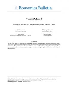
It is well known (see e.g. Deaton and Muellbauer, 1980: chapter 7) that -∆Pp ≥ ∆v ≥ -∆Lp, with strict inequalities unless in the very special case of zero substitution effects, where - ∆v = v(puι) – v(p*) is the Hicksian equivalent variation. Thus, ∆Lp ≤ 0 is a sufficient condition for a consumer surplus (and then a welfare, in this setting) increase, while ∆Pp ≤ 0 is necessary for such a result.1 To illustrate the weakness of the output criterion, consider the case (dual to the one considered by the classic literature) which arises if demands have the same elasticity at the uniform price pu. Intuition suggests that the monopolist should then be willing to make prices to reflect cost differences. Moreover, one can show that, if demands are concave, puι minimizes v(p) over the set {p Σiqi(pi) ≥ Σiqi(pu)}. Thus, any differentiated price vector actually chosen by a profit-maximising monopolist without decreasing total output (as it happens in the linear case) would actually increase consumer surplus, and accordingly social welfare. In the 2-goods case the situation is depicted in Figure 1, where ∆Q = 0 indicates the locus of prices which corresponds to the same total output Σiqi(pu), and V = v(puι) is the relevant consumer surplus indifference curve. The vector q(puι) = [q1(pu), q2(pu)] is orthogonal to the plane ∆Q = 0 due to the assumption of equal demand elasticities, while the price locus ∆Lp = 0 just describes the tangent to V = v(puι) at puι. This property of the uniform pricing might come as a surprise, but it is just due to the substitution effect.
1
While we restrict our attention to the case of monopolistic pricing, it is worth stressing that these properties and the bounds in (1) are completely general. Thus they would apply as well to a setting (in which the assumption of cost differences would perhaps be even more natural) having different firms (imperfectly) competing across markets.
2
Figure 1: Uniform pricing with concave demands, equal demand elasticites at pu p2
V = v(puι)
∆Q = 0 p
q(puι)
u
∆Lp = 0 p1
pu
The situation is less clear-cut if demands are convex: however, consider the case in which demands are isoelastic, i.e., qi(pi) = ki pi− ε , with ki > 0 and εi > 1 (i = 1, …, N).2 It can be shown that, under the assumption of equal demand elasticities (εi = ε, i = 1, ..., N), ∆Lp = 0: see Bertoletti (2007: Appendix B). Accordingly, in such a case monopolistic price differentiation increases total output (by demand convexity, ∆Q = 0 must lie above ∆Lp = 0), aggregate consumer surplus and welfare. Indeed, one can also prove that, when elasticities are the same at puι, if the monopolistic departure from uniform pricing is “small” and output does not decrease, a welfare improvement is generally (whatever demand concavity) achieved: again see Bertoletti (2007: section II).
3. Two linear examples Following Varian (1985: pp. 873-4), one can show that the right-hand side of (1) can be written (under monopolistic pricing): Σici∆qi/(εi(pi*) – 1), with εi(pi) = - qi’(pi)pi/qi(pi), and that for concave demand functions ∆Pp ≤ 0 is a sufficient condition for it being non negative. In fact, in the case of a linear demand system the welfare bounds in (1) become -∆C ≥ ∆W ≥ -∆Pp. Thus, it turns out that we can replace the invalid output test with the checking of the price variations ∆Lp and ∆Pp. Negative value for those variations are indeed sufficient conditions (the latter requires demand concavity) respectively for even a consumer surplus or just a welfare improvement. Note that their verification does not need knowledge of either costs or elasticities.3
2
It is known that in such a case price discrimination under a common marginal cost increases total output: see e.g. Aguirre (2006). 3 It is worth noting that the actual computation of these price variations is common practice in the industries regulated by price caps: see e.g. Armstrong and Sappington (2007: section 3).
3
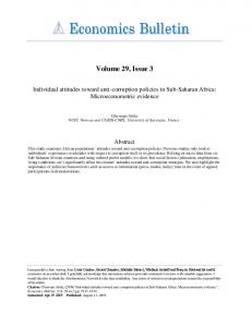
Of course, in the linear case one can compute the prices chosen by the monopolist: it is easily obtained that pu = (Cov{ci,bi} + a + bc)/(2b) and pi* = (ai + bici)/(2bi), where qi(pi) = ai - bipi (ai,bi > 0, ai/bi > ci, i = 1, ..., N), Cov{ci,bi} = (Σicibi)/N – cb is the covariance between ci and bi across markets, and a = (Σiai)/N, b = (Σibi)/N and c = (Σici)/N are respectively the average value of ai, bi and ci. Note that the previous expressions imply that the average value of -bi∆pi = ∆qi is null. Also notice that (pi* - ci) = ai/(2bi) - ci/2. It seems impossible to draw general welfare conclusions: however, if the demand parameters are uncorrelated with the marginal costs (perhaps the interesting case), monopolistic price differentiation implies ∆C < 0 (unless there is no cost variability at all): see Bertoletti (2007: Appendix C). Example 1) A simple case arises if ai/bi is the same across markets, that is exactly the case in which demands have the same elasticity at the uniform price pu. In that case (pi* - pj*) = (ci - cj)/2 and thus the only reason for monopolistic price differentiation is to reflect the marginal cost differences (in the classic setting with a marginal cost common across markets, one gets pu = pi* and allowing price differentiation has no effect at all). Assuming that there exists some marginal cost difference (no matter how small), it turns out that ∆Pp = ∆C/2 < 0 and ∆Lp = 0 (see Bertoletti, 2007: Appendix C): thus, monopolistic price flexibility4 increases both welfare and consumers surplus. Example 2) A special case arises if ai/bi - ci = 2ρ, i = 1, ..., N. In such a case ∆Pp = 0 (note that ci/(εi(pi*) – 1) = (pi* - ci) = ρ, i = 1, ..., N); in fact, one can show that ∆C < 0 and ∆W = ∆π/2 = - ∆v > 0, unless there is no market variability at all and p* = puι. The reason is simple: in this case the Ramsey price vector p* satisfies the second-best conditions we mentioned in section I, and thus p* maximizes W(p) over the set {p Q(p) = Q(puι)}.5 But, at the same time, p* minimizes v(p) over the previous set, since it equalizes qi/qi’ across markets. The situation is illustrated in Figure 2 for the two-markets case.
Figure 2: “Second-best” monopolistic price differentiation pw
∆Q = 0 45°
u
pu
Π dσ
pw * cw
W
V = v(p*)
f
cs pu
4 5
ps*
ps
Notice the prices pi* are discriminatory according to both definitions we mentioned in section I. However, prices pi* are still discriminatory according to the Stigler’s (1987) definition quoted in section I.
4
Without loss of generality, let ps* > pu > pw*, with w,s = 1,2, w ≠ s. Points u, d, f indicate respectively uniform pricing, unconstrained monopolistic pricing and first-best prices. We show three iso-welfare loci (surrounding f) indicated by W and a single iso-profit locus (surrounding d) indicated by Π. Notice that the ∆Q = 0 plane is steeper than the relevant welfare locus at u, while they are tangent at σ (thus ps – pw = cs - cw at that point). Also notice that points d and σ coincide.6 The line fd is the locus of the Ramsey price vectors. This case illustrates the potential conflict between welfare and consumer surplus concerns, but it requires a good deal of demand and cost parameter cross correlation, which is hardly plausible.
References Aguirre, I. (2006) "Monopolistic Price Discrimination and Output Effect under Conditions of Constant Elasticity Demand," Economics Bulletin 4, 1-6. Aguirre, Iñaki (2008) “Joan Robinson Was Almost Right: Output under Third-Degree Price Discrimination” mimeo, Universidad del País Vasco: . Armstrong, M. and D. Sappington (2007) “Recent Developments in the Theory of Regulation” chapter 1 in Handbook of Industrial Organization, Vol. III by M. Armstrong and R. Porter, Eds., Elsevier: Amsterdam. Bertoletti, Paolo (2007) “Monopolistic Price Flexibility and Social Welfare: The Linear Case” mimeo, Pavia University: . Cabral, L.M.B. (2000) Introduction to Industrial Organization, MIT Press: Cambridge (USA). Clerides, S.K. (2004) “Price Discrimination with Differentiated Products: Definition and Identification” Economic Inquiry 42, 402-412. Cowan, Simon and John Vickers (2007) “Output and Welfare Effects in the Classic Monopoly Price Discrimination Problem”, Oxford University, Department of Economics Discussion Paper Series number 355. Deaton, A. and J. Muellbauer (1980) Economics and Consumer Behavior, Cambridge University Press: Cambridge (UK). Schmalensee, R. (1981) “Output and Welfare Implications of Monopolistic Third-Degree Price Discrimination” American Economic Review 71, 242-7. Schwartz, M. (1990) “Third-Degree Price Discrimination and Output: Generalizing a Welfare Result” American Economic Review 80, 1259-62. Stigler, G. (1987) Theory of Prices, McMillan: New York. Varian, H.R. (1985) “Price Discrimination and Social Welfare” American Economic Review 75, 870-5. Varian, H.R. (1989) “Price Discrimination” chapter 10 in Handbook of Industrial Organization, Vol. I by R. Schmalensee and R.D. Willig, Eds., North-Holland: Amsterdam.
With equal marginal costs f would lie along the 45° line and u and σ would coincide. On the contrary, with equal elasticities at pu (and different marginal costs) point d would lie between u and σ and would welfare dominate u. 6
5


![Volume 29, Issue 4 - AccessEcon.com [PDF]](https://m.moam.info/img/260x300/volume-29-issue-4-accesseconcom-pdf_647992eb098a9e92458b4575.jpg)